SFB 649 Discussion Paper 2016-033
Functional Principal
Component Analysis
for Derivatives of
Multivariate Curves
Maria Grith*
Wolfgang K. Härdle*
Alois Kneip*²
Heiko Wagner*²
* Humboldt-Universität zu Berlin, Germany
*² Rheinische Friedrich-Wilhelms-Universität Bonn, Germany
This research was supported by the Deutsche
Forschungsgemeinschaft through the SFB 649 "Economic Risk". http://sfb649.wiwi.hu-berlin.de ISSN 1860-5664
SFB
6
4
9
E
C
O
N
O
M
I
C
R
I
S
K
B
E
R
L
I
N
Functional Principal Component Analysis
for Derivatives of Multivariate Curves
?
Maria Grith,1Wolfgang K. Härdle,1,2Alois Kneip3and Heiko Wagner3
1Ladislaus von Bortkiewicz Chair of Statistics and C.A.S.E. - Center for Applied Statistics and Economics, School of Business
and Economics, Humboldt-Universität zu Berlin, Spandauer Straße 1, 10178 Berlin, Germany
2Sim Kee Boon Institute for Financial Economics, Singapore Management University, 81 Victoria Street, Singapore 188065 3Institute for Financial Economics and Statistics, Department of Economics, Rheinische Friedrich-Wilhelms-Universität Bonn,
Adenauerallee 24-26, 53113 Bonn
Abstract
We present two methods based on functional principal component analysis (FPCA) for the es-timation of smooth derivatives of a sample of random functions, which are observed in a more than one-dimensional domain. We apply eigenvalue decomposition to a) the dual covariance matrix of the derivatives, and b) the dual covariance matrix of the observed curves. To handle noisy data from discrete observations, we rely on local polynomial regressions. If curves are contained in a finite-dimensional function space, the second method performs better asymp-totically. We apply our methodology in a simulation and empirical study, in which we estimate state price density (SPD) surfaces from call option prices. We identify three main components, which can be interpreted as volatility, skewness and tail factors. We also find evidence for term structure variation.
Keywords: functional principal component, dual method, derivatives, multivariate functions, state price densities
JEL codes: C13, C14, G13
?Financial support from the German Research Foundation for the joint project no. 70102424
"Func-tional Principal Components for Derivatives and Higher Dimensions", between Humboldt-Universität zu Berlin and Rheinische Friedrich-Wilhelms-Universität Bonn, is gratefully acknowledged. We would like to thank as well the Collaborative Research Center 649 “Economic Risk” for providing the data and the International Research Training Group (IRTG) 1792 “High-Dimensional Non-Stationary Time Series Analysis”, Humboldt-Universität zu Berlin for additional funding.
1
Introduction
Over the last two decades functional data analysis became a popular tool to handle data entities that are random functions. Usually, discrete and noisy versions of them are observed. Oftentimes, these entities are multivariate functions, i.e., functions with more than one-dimensional domain. Examples include brain activity recordings gen-erated during fMRI or EEG experiments (van Bömmel et al.(2014),Majer et al.(2015)). In a variety of applications though, the object of interest is not directly observable but can be recovered from the observed data by means of derivative. Typical examples of financial applications are functionals retrieved from the observed prices, such as implied risk neutral or state price density (Grith et al.(2012)), pricing kernel (Grith et al.(2013)) or market price of risk (Härdle and Lopez-Cabrera(2012)). Motivated by such data analysis situations, we address the problem of estimating derivatives of multivariate functions from existing discrete and noisy data.
Functions, which are objects of an infinite-dimensional vector space, require spe-cific methods that allow a good approximation of their variability with a small number of components. FPCA is a convenient tool to address this task because it allows us to explain complicated data structures with only a few orthogonal principal components
that fulfill the optimal basis property in terms of itsL2accuracy. These components
are given by the Karhunen-Loève theorem, see for instanceBosq(2000). In addition,
the corresponding principal loadings to this basis system can be used to study the variability of the observed phenomena. An important contribution in the treatment
of the finite-dimensional PCA was done byDauxois et al.(1982), followed by
subse-quent studies that fostered the applicability of the method to samples of observed
noisy curves.Besse and Ramsay(1986), among others, derived theoretical results for
observations that are affected by additive errors. Some of the most important
contri-butions for the extension of the PCA to functional data belong toCardot et al.(1999),
Cardot et al.(2007),Ferraty and Vieu(2006),Mas(2002) andMas(2008). Simple, one-dimensional spatial curves are well understood from both numerical and theoretical perspectives and FPCA is easy to implement in this case. Multivariate objects, with more complicated spatial and temporal correlation structures, or not directly observ-able functions of these objects, such as derivatives, lack a sound theoretical frame-work. Furthermore, computational issues are considerable in higher-dimensional do-main.
To our best knowledge, FPCA for derivatives has been tackled byHall et al.(2009)
andLiu and Müller(2009). The first study handles one-dimensional directional deriva-tives and gradients. The second paper analyses a particular setup in one-dimensional domain where the observations are sparse. This method is applicable to non-sparse data but can be computationally inefficient when dealing with large amounts of ob-servations per curve. For the study of observed functions, there are a series of
empiri-cal studies for the two-dimensional domain case, seeCont and da Fonseca(2002) for
an application close to our empirical study. Further proposals to implement FPCA in more than two dimensions to analyze functions, rather than their derivatives, have
been done particularly in the area of brain imaging, see for instance,Zipunnikov et al.
(2011) who implement multilevel FPCA (Staicu and Carroll(2010),Di et al.(2009)) to analyze brain images of different groups of individuals. However, a thorough deriva-tion of statistical properties of the estimators is missing in these works.
In this paper, we aim to fill in the existent gaps in the literature on FPCA for the study of derivatives of multivariate functions. We present two alternative approaches to obtain the derivatives. The paper is organized as follows: the theoretical framework,
estimation procedure and statistical properties are derived through Section2. Our
empirical study in Section3is guided by the estimation and the dynamics analysis
of the option implied state price densities. It includes a simulation study and a real data example.
2
Methodology
2.1 Two approaches to the derivatives of multivariate functions using FPCA
In this section, we review FPCA from a technical point of view and make the reader familiar with our notation.
Let X be a centered smooth random function in L2([0, 1]g), where g denotes
the spatial dimension, with finite second moment R
[0,1]gE
h
X(t)2id t < ∞for t =
(t1, . . . ,tg)>. The underlying dependence structure can be characterized by the
covari-ance functionσ(t,v)def= E£
X(t)X(v)¤
and the corresponding covariance operatorΓ
(Γϑ)(t)= Z
[0,1]gσ(t,v)ϑ(v)d v.
Mercer’s lemma guarantees the existence of a set of eigenvaluesλ1≥λ2≥. . . and a
corresponding system of orthonormal eigenfunctionsγ1,γ2, . . . called functional
prin-cipal components such that
(1) σ(t,v)=
∞
X
r=1
λrγr(t)γr(v),
where the eigenvalues and eigenfunctions satisfy (Γγr)(t) = λrγr(t). Moreover,
P∞
r=1λr =
R
[0,1]gσ(t,t)d t. The Karhunen-Loève decomposition for the random
func-tionX gives (2) X(t)= ∞ X r=1 δrγr(t),
where the loadingsδr are random variables defined asδr =
R [0,1]gX(t)γr(t)d t that satisfyE h δ2 r i =λr, as well asE £ δrδs ¤
=0 forr6=s. Throughout the paper the following
notation for the derivatives of a functionX will be used
(3) X(d)(t)def= ∂ |d| ∂tdX(t)= ∂d1 ∂td1 1 · · · ∂ dg ∂tgdg X(t1, . . .,tg),
ford=(d1, ...,dg)>anddj∈Nthe partial derivative in the spatial directionj=1, . . .,g.
We denote|d| =Pg
j=1|dj|and require thatX is at least|d| +1 times continuously
dif-ferentiable.
Building on equations (1) and (2), we consider two approaches to model a
de-composition for derivatives X(d). The first one is stated in terms of the
E
h
X(d)(t)X(d)(v)iandλ(1d)≥λ(2d)≥. . . be the corresponding eigenvalues. The prin-cipal componentsϕ(rd),r=1, 2, . . . are solutions to
(4)
Z
[0,1]gσ
(d)(t,v)ϕ(d)
r (v)d v=λr(d)ϕ(rd)(t).
For nonderivatives|d| =0, we introduce the following notationϕ(0)r (t)≡γr(t).
Sim-ilarly to equation (2), the decomposition of X(d)in terms of principal components
ϕ(d) r (t) is given by (5) X(d)(t)= ∞ X r=1 δ(d) r ϕ(rd)(t), forδ(rd)= R [0,1]gX(d)(t)ϕ(rd)(t)d t.
A different way to think about a decomposition for derivatives, is to take the deriva-tives of the functional principal components in (2)
(6) X(d)(t)=
∞
X
r=1
δrγ(rd)(t),
where thed-th derivative of ther-th eigenfunction is the solution to (7) Z [0,1]g ∂|d| ∂vd ¡ σ(t,v)γr(v) ¢ d v=λrγ(rd)(t).
In general, for|d| >0 it holds thatϕ(rd)(t)6=γ(rd)(t), but both basis systems span
the same function space. In particular, there always exists a projection with ar p =
D γ(d)
p ,ϕ(rd)
E =R
[0,1]gγ(pd)(t)ϕ(rd)(t)d tsuch thatPr∞=1ar pϕ(rd)(t)=γ(pd)(t). However, if we
consider a truncation of (2) after a finite number of components this is no longer true in general. An advantage of usingϕ(rd)instead ofγ(rd)is that the decomposition gives
orthonormal basis that fulfill the best basis property, such that for any fixedL∈Nand
every other orthonormal basis systemϕ0
(8) E||X(d)− L X r=1 D X(d),ϕ(rd)Eϕr(d)|| ≤E||X(d)− L X r=1 D X(d),ϕ0rEϕ0r||.
This guarantees that by usingϕ(rd),r =1, . . .,Lwe always achieve the bestL
dimen-sional subset selection in terms of theL2error function. In the next section we show
that estimating the basis functions with such property comes at the cost of inferior
rate of convergence. However, if the true underlying structure lies in aL-dimensional
function space, which is equivalent to a factor model setup, the advantage of
deriv-ing the bestL-orthogonal basis vanishes, because it is possible to derive a basis
sys-tem with the same features using span(γ(d)). This is achieved by performing a spectral decomposition of the finite-dimensional function space ofγ(rd),r=1, . . .,Lto get an orthonormal basis system fulfilling (8).
2.2 Sample inference
Let X1, . . .,XN ∈L2([0, 1]g) be a sample of i.i.d. realizations of the smooth random
Ncurves is given by the sample counterpart (9) σˆ(d)(t,v)= 1 N N X i=1 Xi(d)(t)Xi(d)(v) and for the covariance operator by
(10) Γˆ(Nd)ϕˆ(rd)(t)=
Z
[0,1]gσˆ
(d)(t,v) ˆϕ(d) r (v)d v,
where the eigenfunction ˆϕ(rd)corresponds to the r-th eigenvalue of ˆΓ(Nd). For infer-ence, it holds that||ϕ(rν)−ϕˆr(ν)|| =Op(N−1/2) and|λ(rν)−λˆr(ν)| =Op(N−1/2), see for
in-stanceDauxois et al.(1982) orHall and Hosseini-Nasab(2006). The loadings
corre-sponding to each realizationXi can be estimated via the empirical eigenfunctions as
ˆ δ(d) r i = R [0,1]gXi(d)(t) ˆϕ(rd)(t)d t. 2.3 The model
In most applications, the curves are only observed at discrete points and data is noisy. To model these aspects, we assume that each curve in the sample is observed at inde-pendent randomly-distributed pointsti =(ti1, . . .,ti Ti)>,ti k∈[0, 1]
g,k=1, . . .,T i,i=
1, . . .,N from a continuous distribution with density f such that inf
t∈[0,1]gf(t)>0. We assume that (11) Yi(ti k)=Xi(ti k)+εi k= ∞ X r=1 δr iγr(ti k)+εi k,
whereεi k are i.i.d. random variables withE£εi k¤=0, Var¡ εi k
¢
=σ2iεandεi k is inde-pendent ofXi.
2.4 Estimation procedure
1. Dual method— An alternative to the Karhunen-Loève decomposition relies on the duality relation between the row and column space. The method was first used
in a functional context byKneip and Utikal(2001) to estimate density functions and
later adapted byBenko et al.(2009) for general functions. Letν=(ν1, . . .,νg)>, νj∈N,
|ν| <ρ≤mandM(ν)be the dual matrix of ˆσ(ν)(t,v) from (9) consisting of entries
(12) Mi j(ν)= Z [0,1]gX (ν) i (t)X (ν) j (t)d t.
Letlr(ν)be the eigenvalues of matrixM(ν)andpr(ν)=(p1(νr), . . . ,p(N rν)) be the correspond-ing eigenvectors. Forν=d, the estimators for the quantities in the right-hand side of equations (4) and (5) are given by
(13) ϕˆ(rd)(t)=q1 lr(d) N X i=1 p(i rd)Xi(d)(t) , ˆλ(rd)=l (d) r N and ˆδ (d) r i = q lr(d)p(i rd).
Important for the representation given in equation (6) are the eigenvalues and eigen-vectors ofM(0) denoted bylr def= lr(0),pr def= p(0)r and the corresponding orthonormal
basis ˆγrdef= ϕˆ(0)r and loadings ˆδr idef= δˆ(0)r i. It is straightforward to derive
(14) γˆ(rd)(t)=p1 lr N X i=1 pi rXi(d)(t).
2. Quadratic integrated regression— Before deriving estimators ofM(0)andM(d)
using the model from Section2.3, we outline some results needed to construct these
estimators. For any vectorsa,b∈Rg andc∈Ng, we define|a|def= Pg
j=1|aj|,a−1 def= (a−1 1 , . . .,a−g1)>,ab def = ab1 1 ×. . .×a bg g ,a◦b def =(a1b1, . . .,agbg)>andc!def=c1!×. . .×cg!.
Consider a curveY observed at pointst=©t1, . . . ,tT
ª
, generated as in equation (11). Letk=(k1, . . .,kg)>,kl ∈Nand consider a multivariate local polynomial estimator
ˆ β(t)∈Rρthat solves (15) min β(t) T X l=1 Y(tl)− X 0≤|k|≤ρ βk(t)(tl−t)k 2 KB(tl−t).
KB is any non-negative, symmetric and bounded multivariate kernel function andB
ag×g bandwidth matrix. For simplicity, we assume thatBhas main diagonal entries
b=(b1, . . .,bg)>and zero elsewhere.
As noted byFan et al.(1997) the solution of the minimization problem (15) can also be represented using a weight functionWνT, see Appendix5.2, such that
(16) Xˆb(ν)(t)=ν! ˆβν(t)=ν! T X l=1 WνT³(tl−t)◦b−1 ´ Y(tl).
Local polynomial regression estimators are better suited to estimate integrals like
(12) than other kernel estimators, e.g., Nadaraya-Watson or Gasser-Müller estimator,
since the bias and variance are of the same order of magnitude near the boundary as well as in the interior, see for instanceFan and Gijbels(1992). We propose the
follow-ing estimator for the squared integrated functionsR
[0,1]gX(ν)(t)2d t θν,ρ= Z [0,1]gν! 2XT k=1 T X l=1 WνT³(tk−t)◦b−1 ´ WνT³(tl−t)◦b−1 ´ Y(tl)Y(tk)d t −ν!2σˆ2ε Z [0,1]g T X k=1 WνT³(tk−t)◦b−1 ´2 d t. (17)
where ˆσ2εis a consistent estimator ofσ2ε. The second term is introduced to cancel the bias inE
h
Y2(tk)
i
=X(tk)2+σ2ε.
Lemma 2.1 Under Assumptions5.1-5.4, X is m ≥2|ν|times continuously
differen-tiable, the local polynomial regression is of orderρwith|ν| ≤ρ<m and|σˆ2ε−σ2ε| = OP(T−1/2). As T→ ∞andmax(b)ρ+1b−ν→0,T blog(1×...T×)bg →0as T b1×. . .×bgb4ν→ ∞
Et,Y h θν,ρ i − Z [0,1]gX (ν)(t)2d t=O p à max(b)ρ+1b−ν+ 1 T3/2(b2νb1×. . .×bg) ! Vart,Y(θν,ρ)=Op à 1 T2b 1×. . .×bgb4ν+ 1 T ! , (18)
whereEt,Y denotes the conditional expectation and Vart,Y the conditional variance
givent,Y. The proof of Lemma2.1is given in Appendix5.2.
3. Estimation of M(0)and M(d)— The curvesYi in equation (11) are assumed to be
observed at different random points. For uniformly sampled pointst1, . . .,tT∈[0, 1]g
withT= min
i∈1,...,NTi, we replace the integrals in (17) with the Riemann sums, such that
ˆ Mi j(ν)= ν!2PTi k=1 PTj l=1w T ν(ti k,tj l,b)Yj(tj l)Yi(ti k) ifi6=j ν!2³PTi k=1 PTi l=1w T ν(ti k,ti l,b)Yi(ti l)Yi(ti k)−σˆi2εPTki=1wνT(ti k,ti k,b) ´ ifi=j. wherewνT(ti k,tj l,b) :=T−1PTm=1WνT ³ (ti k−tm)◦b−1 ´ WνT ³ (tj l−tm)◦b−1 ´ . The esti-mator forM(0)is given by settingν=(0, . . ., 0)>and the estimator forM(d)byν=d.
There are two possible sources of error in the construction of the estimator ˆM(ν). One is coming from smoothing noisy curves at a common grid, and has been analyzed in Lemma (2.1). The other one is from approximating the integral in (17) by a sum, see
equation above. In Appendix (5.3) we show that the error of the integral
approxima-tion is of orderT−1/2.
Proposition 2.2 Under the requirements of Lemma2.1
|Mi j(ν)−Mˆi j(ν)| =OP max(b)ρ+1b−ν+ Ã 1 T2b1×. . .×bgb4ν+ 1 T !1/2 .
By Proposition2.2, estimatingM(d)gives an asymptotic higher bias and also a higher
variance than estimatingM(0). This effect becomes more pronounced in higher
di-mensional domain. However, by using local polynomial regression with large
polyno-mial orderρone can still get parametric rates within each method.
Remark 2.3 Under the assumptions of Lemma2.1and using Proposition2.2we can
estimate M(ν)such that if m>ρ≥ g2−1+3Pg
l=1νl, b=T−αwith 1 2(ρ+1−Pg l=1νl)≤α≤ 1 g+4Pg l=1νl then|Mi j(ν)−Mˆi j(ν)| =OP(1/ p T).
We can see that the orders of polynomial expansion and the bandwidths for estimat-ingM(ν)will differ forν=(0, . . ., 0)>andν=d. In particular, the estimator ofM(d)
re-quires higher smoothness assumptions viam>ρ, and a higher bandwidth to achieve
the same parametric convergence rate as the estimator forM(0).
In Lemma2.1it is required that|σ2iε−σˆ2iε| =Op(T−1/2), which ensures
paramet-ric rates of convergence for ˆM(ν)under the conditions of Remark2.3. By Assumption
5.2, in the univariate case, a simple class of estimators forσ2iε, which achieve the
de-sired convergence rate, are given by successive differentiation, seevon Neumann et al.
(1941) andRice(1984). However, as pointed out inMunk et al.(2005), difference
esti-mators are no longer consistent forg≥4 due to the curse of dimensionality. A
possi-ble solution is to generalize the kernel based variance estimator proposed byHall and
Marron(1990) for the multidimensional domain
(19) σˆ2iε= 1 vi Ti X l=1 Yi(ti l)− Ti X k=1 wi l kY(ti k) 2 ,
wherewi l k=Kr,H(ti l−ti k)/PTki=1Kr,H(ti l−ti k) andvi=Ti−2Plwi l k+Pl,kwi l k2 and
Kr,H is ag-dimensional product kernel of orderr with bandwidth matrixH.Munk
et al.(2005) show that if 4r >g and if the elements of the diagonal matrixH are of orderO(T−2/(4r+g)) then the estimator ˆσεi in equation (19) achieves parametric rates
of convergence.
Note that if the curves are observed at a common random grid with T =Ti =
Tj,i,j=1, . . .,N, a simple estimator forM(0)is constructed by replacing the integrals
with Riemann sums in (12). This estimator is given by
˜ Mi j(0)= 1 T PT l=1Yi(tl)Yj(tl) ifi6=j 1 T PT k=1Yi(tl) 2−σˆ2 iεifi=j . (20)
In Appendix (5.3) we verify that the convergence rate of ˜Mi j(0)does not depend ong. When working with more than one spatial dimension, in practice data is often
recorded using an equidistant grid withTpoints in each direction. For our approach,
this strategy will not improve the convergence rate of ˜M(0)due to the curse of
dimen-sionality. If it is possible to influence how data is recorded, we recommend using a common random grid, which keeps computing time and the storage space for data to a minimum and still gives parametric convergence rates for the estimator ofMi j(0).
IfT ÀN equation (20), gives a straightforward explanation why the dual matrix is
preferable to derive the eigendecomposition of the covariance operator, because tak-ing sums has a computational cost that is linear.
4. Estimating the basis functions— We keep notationsν=d to refer to the spec-ification in equation (5) andν=(0, . . ., 0)>to (6). A spectral decomposition of ˆM(ν)
is applied to obtain the eigenvalues ˆlr(ν)and eigenvectors ˆpr(ν)forr,j =1, . . .,N. This
gives straightforward empirical counterparts ˆλ(rν,T)=lˆr(ν)/Nand ˆδ(r jν),T= q
ˆ
lr(ν)pˆ(r jν). To estimateϕ(rd) andγ(rd), a suitable estimator for Xi(d),r,j =1, . . .,N is needed.
We use a local polynomial kernel estimator, denoted ˆXi(,dh), similarly to (16), with a polynomial of orderpand bandwidth vectorh=(h1, . . .,hg). Here,his not equal to
b, the bandwidth used to smooth the entries of the ˆM(0)and ˆM(d)matrix. In fact, we
show below that the optimal order for the bandwidth vectorhdiffers asymptotically
from that ofbderived in the previous section. An advantage of using local polynomial
estimators, compared for example to spline or wavelet estimators, is that the bias and variance can be derived analytically. For the univariate case these results can be found inFan and Gijbels(1996) and for the multivariate case inMasry(1996) andGu et al.
(2015). We summarize them in terms of order of convergence below
Et,Y h Xj(d)(t)−Xˆj(d,h)(t) i =Op(max(h)p+1h−d) Vart,Y ³ ˆ X(jd,h)(t)´=Op à 1 T h1×. . .×hgh2d ! . (21)
Using these results, it follows that for max(h)p+1h−d→0,³max(h)p+1T h−d´−1→0
asT→ ∞andpchosen such thatp− |d|is odd
Et,Y 1 q l(rν) N X i=1 pi r(ν) ³ Xi(d)(t)−Xˆi(d,h)(t) ´ = 1 q lr(ν) N X j=1 p(j rν)Bias ³ ˆ Xj(d,h)(t) ´ +Op ³ max(h)p+1h−d ´ =Op(max(h)p+1h−d) Vart,Y 1 q lr(ν) N X i=1 p(i rν)Xˆi(d,h)(t) = 1 lr(ν) N X j=1 ³ p(j rν)´2Var ³ ˆ X(jd,h)(t) ´ +Op à 1 N T h1×. . .×hgh2d ! =Op à 1 N T h1×. . .×hgh2d ! .
In the next Proposition we show that under certain assumptions the asymptotic mean squared error of ˆϕ(rd,T)and ˆγ(rd,T)is dominated by these two terms.
Proposition 2.4 Under the requirements of Lemma 2.1, Assumptions 5.6 and 5.7,
Remark 2.3, and for inf
s6=r|λr −λs| > 0, r,s = 1, . . .,N and max(h) p+1h−d → 0 with N T h1. . .hgh2d→ ∞as T,N→ ∞we obtain a) |γ(rd)(t)−γˆ(rd,T)(t)| =Op ³ max(h)p+1h−d ´ +Op ³ (N T h1×. . .×hgh2d)−1/2 ´ b) |ϕˆ(rd)(t)−ϕˆ(rd,T)(t)| =Op ³ max(h)p+1h−d´+Op ³ (N T h1×. . .×hgh2d)−1/2 ´
A proof of Proposition2.4is provided in Appendix5.4. As a consequence, the
result-ing global optimal bandwidth is given byhr,op t =Op
³
(N T)−1/(g+2p+2)
´
. Even if the optimal bandwidth for both approaches and each basis function is of the same order of magnitude, the values of the actual bandwidths may differ. A simple rule of thumb for the choice of bandwidths in practice is given in Section3.1.
2.5 Properties under a factor model structure
Often, the variability of curves can be expressed with only a few basis functions
mod-eled by a truncation of (2) afterLbasis functions. If a true factor model withL
com-ponents is assumed, the basis representation to reconstructX(d)is arbitrary, in the
sense that (22) X(d)(t)= L X r=1 δrγ(rd)(t)= Ld X r=1 δ(d) r ϕ(rd)(t).
HereLis always an upper bound forLd. The reason for this is that by taking derivatives
it is possible thatγ(rd)(t)=0 or that there exits some ar ∈RL−1 such thatγ(rd)(t)=
P
s6=rasrγ(sd)(t).
Based on the methodology described in Section2.4, the two estimators for
deriva-tives are given by (23) Xˆi(,dF PC A) 1(t) def = L X r=1 ˆ δi r,Tγˆ(rd,T)(t) ≈ Xˆi(d,F PC A) 2(t)def= Ld X r=1 ˆ δ(d) i r,Tϕˆ (d) r,T(t).
Proposition 2.5 Assume that a factor model with L factors holds for X . For N T−1→0, together with the requirements of Proposition2.4, the true curves can be reconstructed
a) |Xi(d)(t)−Xˆi(d,F PC A) 1(t)| =Op ³ T−1/2+max(h)p+1h−d+(N T h1×. . .×hgh2d)−1/2 ´ b) |Xi(d)(t)−Xˆi(,dF PC A) 2(t)| =Op ³ T−1/2+max(h)p+1h−d+(N T h 1×. . .×hgh2d)−1/2 ´ .
A proof of Proposition (2.5) is given in Appendix (5.5). Compared with the
conver-gence rates of the individual curves estimators, see (21), the variance of our
estima-tors reduces not only inTbut also inN. Equations (13) and (14) can be interpreted as
an average overNcurves for only a finite number ofLcomponents. The intuition
be-hind it is that only those components are truncated that are related to the error term and thus a more accurate fit is possible. IfNincreases at a certain rate, it is possible to get close to parametric rates. Such rates are not possible when smoothing the curves individually.
For the estimation of ˆXi(d,F PC A)
2, as illustrated in Remark2.3, additional assumptions
on the smoothness of the curves are needed to achieve the same rates of convergence for the estimators ˆM(d) and ˆM(0). With raisingg and|d|it is required that the true curves become much smoother which makes the applicability of estimating ˆXi(d,F PC A)
2
limited for certain applications. In contrast, the estimation ofM(0)still gives almost parametric rates if less smooth curves are assumed. In addition, if the sample size is
small, using a high degree polynomial needed to estimateM(d)might lead to
unre-liable results. To learn more about these issues, we check the performance of both
approaches in a simulation study in Section3.2using different sample sizes.
3
Application to state price densities implied from option prices
In this section we analyze the state price densities (SPDs) implied by the stock in-dex option prices. As state dependent contingent claims, options contain information about the risk factors driving the underlying asset price process and give information about expectations and risk patterns on the market. Mathematically, SPDs are equiv-alent martingale measures for the stock index and their existence is guaranteed in the absence of arbitrage plus some technical conditions. In mathematical-finance ter-minology they are known as risk neutral densities (RNDs). A very restrictive model, with log-normal marginals for the asset price, is the Black-Scholes model. This model results in log-normal SPDs that correspond to a constant implied volatility surface across strikes and maturity. This feature is inconsistent with the empirically
docu-mented volatility smile or skew and the term structure, seeRubinstein(1985).
There-fore, richer specifications for the option dynamics have to be used. Most of earlier works adopt a static viewpoint; they estimate curves separately at different moments
in time, see the methodology reviews byBahra(1997),Jackwerth(1999) andBliss and
Panigirtzoglou(2002). In order to exploit the information content from all data avail-able, it is reasonable to consider them as collection of curves.
The relation between the SPDs and the European call prices has been
demon-strated byBreeden and Litzenberger(1987) andBanz(1978) for a continuum of strike
prices spanning the possible range of future realizations of the underlying asset. For a fixed maturity, the SPD is proportional to the second derivative of the European call
options with respect to the strike price. In this case, SPDs are one-dimensional func-tions. A two-dimensional point of view can be adopted if maturities are taken as an additional argument and the SPDs are viewed as a family of curves.
LetC :R2
≥0→Rdenote the price function of a European call option with strike
pricekand maturityτsuch that
(24) C(k,τ)=exp (−rττ)
Z ∞
0
(sτ−k)+q(sτ,τ)d sτ,
whererτis the annualized risk free interest rate for maturityτ,sτthe unknown price
of the underlying asset at maturity,kthe strike price andqthe state price density of
sτ. One can show that
(25) q(sτ,τ)=exp (rττ)∂ 2C(k,τ) ∂k2 ¯ ¯ ¯ ¯ ¯ k=sτ .
Lets0be the asset price at the moment of pricing and assume it to be fixed. Then by
the no-arbitrage condition, the forward price for maturityτis
(26) Fτ=
Z ∞
0
sτq(sτ,τ)d sτ=s0exp(rττ).
Suppose that the call price is homogeneous of degree one in the strike price. Then
(27) C(k,τ)=FτC(k/Fτ,τ).
If we denotem=k/Fτthe moneyness, it is easy to verify that
(28) ∂ 2C(k,τ) ∂k2 = 1 Fτ ∂2C(m,τ) ∂m2 .
Then one can show that ford=(2, 0)>,C(d)(m,τ)|m=sτ/Fτ=q(sτ/s0,τ)=s0q(sτ,τ). In
practice, it is preferable to work with densities of returns instead of prices when ana-lyzing them jointly because prices are not stationary. Also, notice that call price curves
are not centered. This leads to an additional additive term in equations (4) and (6),
which refers to the population mean. We show in the next section how to handle this in practice. For our application,Xwill refer to the rescaled call priceC(m,τ). Therein, we also assume that the indexi=1, . . . ,Nrefers to ordered time-points.
The code used to generate the results reported in this section is published online at www.github.com/QuantLet/FPCA and www.quantlet.de. The data used in the em-pirical study is available from the authors upon request.
3.1 Implementation
1. Centering the observed curves — Throughout the paper it is assumed that the curves are centered. To satisfy this assumption, we subtract the empirical mean
¯
X(ν)(tk) = N1PNi=1Xˆi(,νb)(tk) from the the observed call prices to obtained centered
curves. A centered versionM(ν),ν=(0,d) is given by (29) M(i jν)=Mˆi j(ν)− 1 T T X k=1 ³ ¯ X(ν)(tk) ˆXi(ν,b)(tk)+X¯(ν)(tk) ˆX(jν,b)(tk)−X¯(ν)(tk)2 ´ .
It is still possible to improve the centering the curves. One possibility is to use a dif-ferent bandwidth to compute the mean because averaging will necessarily lower the variance. Secondly, by the arguments of Section2.4, the T1PT
k=1X¯(ν)(tk)2term can be
improved accordingly to Lemma2.1by subtracting ˆσεweighted by suitable
parame-ters. We decide to omit these fine tunings in our application because it would involve a significant amount of additional computational effort for only minor improvements.
2. Bandwidth selection— To get parametric rates of convergence for ˆM(d)related to Remark2.3we chooseρ=7 andbbetweenO(T−1/10) andO(T−1/12). The choice
ofb to estimate ˆM(0) is similar, with the difference thatρ>0, we chooseρ=1 and
b has to lie betweenO(T−1/3) andO(T−1/5). We use a simple criteria to choose the
bandwidth because by Proposition2.4the dominating error depends mainly on the
choice ofh. Letti k=(ti k1, . . .ti kg), then the bandwidth for direction j is determined
bybj =
³
(maxk(ti k j)−mink(ti k j))Ti
´α
. When estimating state price densitiesti k =
(τi k,mi k) andTi is replaced by the cardinality ofτi={τi1, . . .τi Ti} andmi respectively.
In the estimation of ˆM(d)we setα= −1/10 andα= −1/3 for ˆM(0).
The choice of bandwidthshis a crucial parameter for the quality of the estimators.
To derive an estimator for the bandwidths first note that in the univariate case (g=1)
the theoretical optimal univariate asymptotic bandwidth for ther-th basis is given by
(30) hdr,,op tν =Cd,p(K) T−1 R1 0 PN i=1(p (ν) i r )2σ2εi(t)fi(t)−1d t R1 0 n PN i=1p (ν) i r X (p+1) i (t) o2 d t 1/(2p+3) , Cd,p(K)= (p+1)!2(2d+1)R K∗2 p,dj(t)d t 2(p+1−d){R up+1K∗ d,p(t)d t}2 1/(2p+3) .
Like in the conventional local polynomial smoothing caseCd,p(K) does not depend
on the curves and is an easily computable constant. It only depends on the chosen kernel, the order of the derivative and the order of the polynomial, see for instance
Fan and Gijbels(1996).
For our bandwidth estimator we treat every dimension separately, similar to choos-ing an optimal an optimal bandwidth for derivatives in the univariate case, and
cor-rect for the asymptotic order, see Section2.4. In practice, we can not use equation
(30) to determine the optimal bandwidth because some variables are unknown and
only discrete points are observed. As a rule-of-thumb, we replace these unknown vari-ables with empirical quantities: estimates of pi r(0) from ˆM(0) and ofpi r(d) from ˆM(d). With these approximations, a feasible rule for computing the optimal bandwidth in directionj for ther-th basis functionhj r is given by
(31) hdj r,ν,r ot= T−1 Cd2p,p+3σˆ2ε fjR01 n PN i=1pˆ (ν) i r X˜ (p+1) i (tj) o2 d tj 1/(g+2p+2) .
In our application as well as our simulation we haveg =2,d =(0, 2) and do a third
• The density of the observed points is approximated by a uniform distribution withf1=maxi,j(τi j)−mini,j(τi j) andf2=maxi,j(mi j)−mini,j(mi j).
• To get a rough estimator forXi(p+1)based on Xi, we use a polynomial
regres-sion. For our application, we takep=3 and are thus interested in estimates for
Xi(4)(m) andXi(4)(τ). We expect the curves to be more complex in the money-ness direction than in the maturity direction and we adjust the degree of the polynomials to reflect this issue. The estimates are then given by
a∗i =arg min ai à Xi(m,τ)−ai0+ 5 X l=1 ai lml+ 9 X l=6 ai lτ(l−5) ! ˜ Xi(4)(m)=24ai∗4+120a∗i5m ˜ Xi(4)(τ)=24ai∗9. (32)
• To estimate the variance for each curve we use the kernel approach given in (19) using a Epanechnikov kernel with a bandwidth ofT−2/(4+g)for each spatial direction. In addition, these estimates are used to correct for the diagonal bias when ˆM(0)and ˆM(d)are estimated. In (31) the average over all ˆσi²is used.
We use the product of Gaussian kernel functions to construct local polynomial
es-timators. We can verify from Proposition2.4that the optimal bandwidthhdecreases
inN. By using a global bandwidth and a compact kernel the matrix given in equation
(45) may become singular whenNis large andT is small.
In our simulation and application we use the mean optimalhdi,,r otν =L−1PL
r=1h d,ν
i r,r ot
for each ˆγ(rd), ˆϕ(rd)to reduce computation time. Since we demean the sample in (29),
finally we addN−1PN
i=1Xˆ (d)
i,hdi,,r otν to the resulting truncated decomposition to derive the
final estimate.
3. Estimation of the number of components— In Section2.5we assumed that the number of components is given. In general, the number of basis functions needed is unknown a priori. For the case|d| =0 there exists a wide range of criteria that can be
adapted to our case to determine the upper boundL. The easiest way to determine
the number of components is by choosing the model accuracy by an amount of
vari-ance explained by the eigenvalues. In (71) we show that under the conditions from
Proposition2.4λˆ(rd)−λˆ(rd,T)=Op(N−1/2T−1/2+T−1) andλ (d)
r −λˆ(rd)=Op(N−1/2). The
as-sumptions in Corollary 1 fromBai and Ng(2002) can be adapted to our case and give
several criteria for findingLorLdby generalizingMallows(1973)Cpcriteria for panel
data settings. These criteria imply minimizing the sum of squared residuals whenk
factors are estimated and penalizing the overfitting. One such formulation suggests choosing the number of factors using the criteria
(33) PC(ν)(k∗)= min k∈N,k≤Lmax à N X r=k+1 ˆ λ(ν) r ! +k à N X r=Lmax ˆ λ(ν) r ! à log(CN T2 ) CN T2 ! ,
for the constantCN T =min(
p
N,pT) and a prespecifiedLmax<min(N,T).Bai and
consider the above modified version (34) IC(ν)(k∗)= min k∈N,k≤L log à 1 N N X r=k+1 ˆ λ(ν) r ! +k à log(C2N T) C2N T ! .
Here usingν=(0, . . ., 0)>will giveLwhile usingν=d will give the factorsL
d.
Another possibility for the choice of number of components is to compute the vari-ance explained by each nonorthogonal basis by
(35) Var( ˆδ(rd,T)γˆ(rd,T))= 〈γˆr(d,T), ˆγr(d,T)〉λˆr.
We can sort the variances in decreasing order and use either equation (33) or (34) to select the number of components.
3.2 Simulation Study
We investigate the finite sample behavior of our estimators in a simulation study,
which is guided by the real data application in Section3.3. Simulated SPDs are
mod-eled as mixtures ofGcomponents,q(m,τ)=PG
l=1wlq
l(m,τ), whereql are fixed
ba-sis functions andwl are random weights. For fixedτwe considerql(·,τ) to be a log-normal density functions, with mean
³
µl−12σ2l
´
τ and variance σ2lτ, and simulate weightswi l withPGl=1wi l=1, wherei=1, . . . ,Nis the index for the day, then
(36) qi(m,τ)= G X l=1 wi l 1 mq2πσ2lτ exp − 1 2 log (m)− ³ µl−12σ2l ´ τ σl p τ 2 .
FollowingBrigo and Mercurio(2002) the prices of call options for these SPDs are
(37) Ci(m,τ)=exp (−riττ) G X l=1 wi l© exp(µlτ)Φ(y1)−mΦ(y2) ª wherey1= log³m−1´ +³µl+12σ 2 l ´ τ σlpτ ,y2= log³m−1´ +³µl−12σ 2 l ´ τ
σlpτ andΦis the standard normal cdf.
This representation corresponds to a factor model in which the mixture components are densities associated with a particular state of nature and the loadings are equiva-lent with probabilities of states.
We illustrate the finite sample behavior forG=3 withµ1=0.4,µ2=0.7,µ3=0.1,
andσ1=0.5,σ2=0.3,σ3=0.3. The loadings are simulated from the positive
half-standard normal distribution, then half-standardized to sum up to one. One can verify that the correlation matrix for the loadings is
R= 1 −0.5 −0.5 −0.5 1 −0.5 −0.5 −0.5 1 ,
which is singular with rank(R)=2. As a result, the covariance operator of the SPD
curves hasL=G−1 nonzero eingenvalues. In this example, using a mixture of three
factors means that only two principal components are necessary to explain the vari-ance in the true curves.
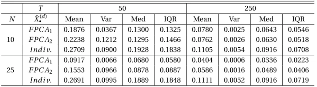
T 50 250
N Xˆ•(d) Mean Var Med IQR Mean Var Med IQR
10 F PC A1 0.1876 0.0367 0.1300 0.1325 0.0780 0.0025 0.0643 0.0546 F PC A2 0.2238 0.1212 0.1295 0.1466 0.0762 0.0026 0.0630 0.0518 I nd i v. 0.2709 0.0900 0.1928 0.1838 0.1105 0.0054 0.0916 0.0708 25 F PC A1 0.0917 0.0066 0.0680 0.0580 0.0404 0.0006 0.0336 0.0223 F PC A2 0.1553 0.0966 0.0878 0.0887 0.0586 0.0016 0.0489 0.0406 I nd i v. 0.2691 0.0995 0.1889 0.1848 0.1111 0.0052 0.0916 0.0719
Table 1.Results of the simulation described in Section3.2with different values forT andN.
F PC A1andF PC A2are superior in sense of MSE over the individual estimation of the derivatives
in each setting.F PC A1is better thanF PC A2except forN=10,T=250. ForF PC A1and
F PC A2the estimation improves with raisingNandT. These results support our asymptotic
results given by Proposition2.2and2.5.
FPCAsimulation
Without loss of generality, we setriτ=0, for each dayi=i, . . . ,N. We construct a random grid for each observed curveXi by simulating pointsti k=(mi k,τi k),k=
1, . . .,T from a uniform distribution with continuous support [0.5, 1.8]×[0.2, 0.7]. Fi-nally, we record noisy discrete observations of the call functions with additive error term i.i.d.εi k∼N(0, 0.12).
The true SPDs given by equation (36) are used to verify the performance of
ˆ
XF PC A(d)
1, ˆX
(d)
F PC A2and of the individually estimated curves ˆX
(d)
I nd i v., in terms of mean
in-tegrated squared error (MSE), i.e.,T−1PT
k=1
n
X(d)(ti k)−Xˆ•(d)(ti k)
o2
, ford=(2, 0). For evaluation we generate a common grid of 256 points from a uniform distribution. To derive the optimal bandwidth in each case we stick to the rule-of-thumb approach
presented in Section3.1. The bandwidth for the individually smoothed curveiis
de-rived by replacing ˆp(i rν)in (31) by one and zero otherwise. The performance is recorded
for sample sizesN of 10 and 25 withT observations per day of size 50 and 250. This
procedure is repeated 500 times to get reliable results, mean, variance and the inter quartile distance based at the MSE of the repetitions are given in Table1.
Both FPCA based approaches give better estimates for the derivative of the call functions than an individually applied local polynomial estimator of the individual curves. Both the mean and the median of the MSE are smaller which is a result of the
additional average overN for the basis functions as given by Proposition2.5.
How-ever, theF PC A1 method performs decisively better for smallT than the other two
both in terms of mean and standard deviation of the mean squared error. In addition
F PC A1benefits more from increasingNthanF PC A2. With smallT forF PC A2and
individual smoothing the variability of MSE is much bigger than forF PC A1while the
median ofF PC A1andF PC A2are comparable. This means individual smoothing and
F PC A2must behave much worse thanF PC A1in some instances whileF PC A1was
able to stabilize the estimates. To get the same effect usingF PC A2a much biggerTis
needed. A possible explanation for this behavior is given by Proposition2.2. The rates
of convergence for the estimators of the dual matrix entries rely onT. Thus in finite
3.3 Real Data Example
1. Data description —We use settlement European call option prices written on the underlying DAX 30 stock index. These prices are computed by EUREX at the close of each trading day as an average of the intraday transaction prices. The data range is ten years, between January 2, 2002 and December 3, 2011, and includes 2557 days. The expiration dates of the options are set on the third Friday of the month. Therefore, on a particular day, option prices with only a few maturities are available, see
Fig-ure1. The distance between two consecutive observed maturities is higher for more
distant expiration dates, while the distance between two consecutive strike prices is relatively constant. Methods that analyze curves jointly are generally better tailored to this type of data, because they provide better estimates at grid points with only a few observations available of the individual curves. We include call options with maturity between one day and one year. The sample contains prices of options with an average of six maturities and sixty-five strikes per day.
By assuming ’sticky’ coordinates for the daily observations, in accordance with
equation (27), we divide the strike and the call prices within one day by the stock
index forward price to ensure that the observation points are in the same range.
Af-terwards, we apply the estimation methodology described in Section2to the rescaled
call prices as a function of moneyness and maturity. Our proxy for the risk-free inter-est rates are the EURIBOR rates, which are listed daily for several maturities. We apply a linear interpolation to calculate the rate values for desired maturities.
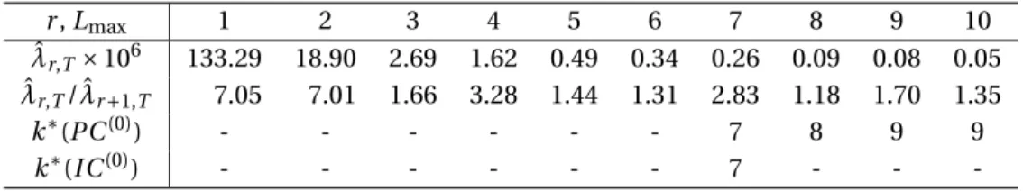
2. Estimation results — We report the results for the loadings estimated by spec-tral decomposition of dual covariance matrix for option price functions, and the es-timates of the second partial derivative of the functional principal components. The first eigenvalue of the dual covariance matrix ˆM(0)for the call option surfaces has a dominant explanatory power. The order of magnitude of the following eigenvalues decreases by a factor of ten for every few additional components. To detect the rela-tive contribution of consecurela-tive components, we construct the ratio of two adjacent
estimated eigenvalues in descending order, seeAhn and Horenstein(2013). The first
two terms are dominating the sequence and there are spikes at the fourth and
sev-enth component ratio.PC(0)criterion suggests at least seven components, see values
ofk∗forLmax≥7 in Table2.IC(0)criterion, which does not depend on the truncation
parameterLmax, suggests seven components.
r,Lmax 1 2 3 4 5 6 7 8 9 10 ˆ λr,T×106 133.29 18.90 2.69 1.62 0.49 0.34 0.26 0.09 0.08 0.05 ˆ λr,T/ ˆλr+1,T 7.05 7.01 1.66 3.28 1.44 1.31 2.83 1.18 1.70 1.35 k∗(PC(0)) - - - - - - 7 8 9 9 k∗(IC(0)) - - - 7 - -
-Table 2. Estimated eigenvalues and eigenvalue ratios. Number of factors byPC(0)criterion
1 0.75 Maturity 0.5 0.25 15-Jun-2007 0 1.5 1.25 1 Moneyness 0.75 0.5 0 0.5 Call prices 1.5 1.25 Moneyness 1 0.75 0.5 0 0.25 0.5 Maturity 0.75 -100 0 100 1 ^ . ( d ) 2 ;T 2002 2004 2006 2008 2010 2012 ^/2;T -0.06 -0.04 -0.02 0
Green: 15-Jun-2007. Red: 18-Jun-2007
1 0.75 Maturity 0.5 0.25 18-Jun-2007 0 1.5 1.25 1 Moneyness 0.75 0.5 0 0.5 Call prices
Figure 1. The effect of expiration date on the level of estimated loadingsδˆ2,T
FPCAexpiration
A closer look at the dynamics of the loadings ˆδ2,T shows an unusual behavior
be-tween mid-February 2007 through mid-June 2008. This interval spans the financial crisis and extends until the end of the recession in the Euro Area, according to the Center for Economic and Policy Research (CEPR) recession indicator. The loadings are extremely volatile and display a particular time regularity of jumps. We identify these jumps with the Mondays following an expiration date (options expire at a monthly frequency, always on a Friday). Figure1highlights the dynamics of ˆδ2,Ton and
follow-ing an expiration day. After roughly two weeks, the loadfollow-ings revert to a ’normal’ level. During this period, for small maturities, there are only few observations available for call prices with strikes larger than the current stock index. In addition, the absence of a call string with close enough time to maturity on the following trading Monday, introduces bias in the estimated smooth call surface for grid values outside the obser-vation points range. The shape of the second estimated component ˆγ(2,dT), displayed in Figure1, suggests that it is related to variations of the short end of the SPD term struc-ture. A similar behavior of the loadings are observed for a few other components we investigated: ˆδ4,T, ˆδ5,Tand ˆδ6,T. Their variances remain important even if we exclude
the interval with large jumps from the sample. The corresponding components have similar shape features to the three components we discuss below. We argue that they impact the option prices and SPDs when jumps in the underlying occur, and that they related to the asymmetric behavior of the option prices along the maturity direction.
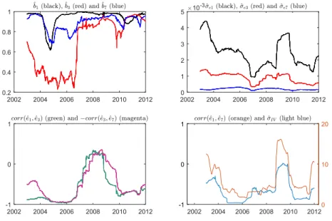
The estimated components ˆγ(1,dT), ˆγ(3,dT) and ˆγ(7,dT) together with their loadings are
dis-played in Figure2. They describe three types of asymmetry present in the dynamics of
the SPDs. The first component, is similar in shape to the empirical mean of the SPD. It has a long left tail, specific to the negatively skewed densities and a peak located at a value of moneyness slightly above one. For positive levels of the loadings, this
compo-1.5 1.25 Moneyness 1 0.75 0.5 0 0.25 0.5 Maturity 0.75 200 0 -200 1 ^ . ( d ) 1 ;T 2002 2004 2006 2008 2010 2012 ^/1;T -0.06 -0.04 -0.02 0 0.02 0.04 1.5 1.25 Moneyness 1 0.75 0.5 0 0.25 0.5 Maturity 0.75 1000 0 -1000 1 ^ . ( d ) 7 ;T 2002 2004 2006 2008 2010 2012 ^/7;T #10-3 -2 -1 0 1 2 1.5 1.25 Moneyness 1 0.75 0.5 0 0.25 0.5 Maturity 0.75 -100 0 100 1 ^ . ( d ) 3 ;T 2002 2004 2006 2008 2010 2012 ^/3;T -0.015 -0.01 -0.005 0 0.005 0.01
Figure 2. Estimated componentsγˆ(d) 1,T,γˆ
(d) 3,Tandγˆ
(d)
7,T and their loadings obtained by the
decomposition of the dual covariance matrixMˆ(0)
FPCAcomponents
nent increases the mass of SPD around the mode and decreases the values in the tails. We find that this component is related to the time-varying volatility of the index re-turns. The next component, ˆγ(3,dT) has a ’valley-hill’ pattern, which shifts mass around the central region of the density. A positive shock in the direction of this components increases the negative skewness, and a large negative shock can reverse the sign of the SPD skewness. This component is interpreted as a skewness factor. The last com-ponent, ˆγ(7,dT) takes negative values in the left tail and displays a prominent positive valued peak at the right of the mode of the empirical SPD mean. This component rep-resents a tail factor, and we show that its loading can be interpreted as the volatility of volatility index.
The functional principal components of the reduced modelP
r∈{1,3,7}δˆr,Tγˆ(rd,T)
re-semble closely the three components displayed in Figure2. Further analysis shows
that when including any additional component to the reduced representation, the shape of the orthogonal basis changes to some extent. The loadings of all orthogo-nalized components become ’contaminated’ with jumps. Moreover, all the loadings estimated by decomposing ˆM(d), ford =(2, 0)>feature the jump-behavior outlined
above, between mid-February 2007 and mid-September 2008. For those reasons, ˆM(0)
decomposition enables a better interpretation of the components, by separating the continuous and discontinuous sources of variation in the SPDs.
We show next that the first estimated component ˆγ(1,dT) is related to the expected
variance under a risk neutral measureQ, which admits the densityq. Under this
mea-sure, the prices are martingales. Equations (6) and (26) yield
(38) E Q i ¡ si+τ/Fi ¢ exp(riττ) = Z ∞ 0 mq˜(m,τ)d m+ ∞ X r=1 δi r Z ∞ 0 mγ(rd)(m,τ)d m=1,
where ˜qis the population mean. The computation of the second moment gives
(39) Var Q i ¡ si+τ/si ¢ exp(riττ)2 = Z ∞ 0 m2q˜(m,τ)d m+ ∞ X r=1 δi r Z ∞ 0 m2γ(rd)(m,τ)d m−1.
We consider the empirical version of Equation (39), forτ=1 month. Instead of
com-puting the integrals, based on our estimates of ˜qandγ(d), we assume them to be un-known coefficients in a linear regression, in which the empirical loadings are used as explanatory variables of the real-data proxy for the standardized variance. In the
nu-merator, we use the squared VDAX index multiplied byτ. This index is computed by
Deutsche Börse AG from the prices of call and put options and reflects market expecta-tion under the risk neutral measure of the 30 day ahead square root implied variance
for the DAX 30 log-returns, which is then annualized.Duan and Yeh(2010) show that
squared volatility index is a good approximation of the expected risk-neutral volatility when the jumps are small. While the volatility index refers to the standard deviation of the log-returns under the risk neutral measure, it can still be used in the regression because the transformationq(logm,τ)=mq(m,τ) maintains the linear-relationship between the dependent and explanatory variables. We find that the most important
component in the regression is ˆδ1,T (adjusted R-squared in the univariate regression
is 93.97%). When including ˆδ3,T as an additional regressor, it increases the adjusted
R-squared to 94.06%, while ˆδ7,T has a negative marginal contribution to the goodness
of fit of multivariate regression.
No skewness index is readily available, and we take a simple measure instead, Pear-son’s skewness coefficient. In terms of equations (38) and (39), for a fixed maturityτ, it is equal to (40) 1−arg max m © q(m,τ)ª q VarQi ¡ si+τ/si ¢ / exp(riττ) .
Since the first component ˆγ(1,dT) is unimodal (as it is also ˆγ(2,dT)), the SPD mode is mostly affected by the loadings of the third component ˆγ(3,dT) (and to some extend by those of the seventh component ˆγ(7,dT)).
3. Dynamic analysis of the loadings — In this section, we investigate the dynam-ics of the loadings in the reduced model. The partial autocorrelation function of all