Do Value-Added Estimates Add Value? Accounting for
Learning Dynamics
Tahir Andrabi
Department of Economics - Pomona College
Jishnu Das
World Bank - Development Economics Research Group (DECRG)
Asim Ijaz Khwaja
John F. Kennedy School of Government - Harvard University
Tristan Zajonc
John F. Kennedy School of Government - Harvard University
Faculty Research Working Papers Series
October 2009
RWP09-034
The views expressed in the HKS Faculty Research Working Paper Seriesare those of the author(s) and do not necessarily reflect those of the John F. Kennedy School of Government or of Harvard University. Faculty Research Working Papers have not undergone formal review and approval. Such papers are included in this series to elicit feedback and to encourage debate on important public policy challenges. Copyright belongs to the author(s). Papers may be downloaded for personal use only.
Policy Research Working Paper
5066
Do Value-Added Estimates Add Value?
Accounting for Learning Dynamics
Tahir Andrabi
Jishnu Das
Asim Ijaz Khwaja
Tristan Zajonc
The World Bank
Development Research Group
Human Development and Public Services Team
September 2009
WPS5066
Public Disclosure Authorized
Public Disclosure Authorized
Public Disclosure Authorized
Abstract
The Policy Research Working Paper Series disseminates the findings of work in progress to encourage the exchange of ideas about development issues. An objective of the series is to get the findings out quickly, even if the presentations are less than fully polished. The papers carry the names of the authors and should be cited accordingly. The findings, interpretations, and conclusions expressed in this paper are entirely those of the authors. They do not necessarily represent the views of the International Bank for Reconstruction and Development/World Bank and its affiliated organizations, or those of the Executive Directors of the World Bank or the governments they represent.
Policy Research Working Paper 5066
Evaluations of educational programs commonly assume that what children learn persists over time. The authors compare learning in Pakistani public and private schools using dynamic panel methods that account for three key empirical challenges to widely used value-added models: imperfect persistence, unobserved student heterogeneity, and measurement error. Their estimates suggest that only a fifth to a half of learning persists between grades
This paper—a product of the Human Development and Public Services Team, Development Research Group—is part of a larger effort in the department to expand our knowledge of child learning and test scores as a broad measure of educational outcomes. Policy Research Working Papers are also posted on the Web at http://econ.worldbank.org. The author may be contacted at [email protected].
and that private schools increase average achievement by 0.25 standard deviations each year. In contrast, estimates from commonly used value-added models significantly understate the impact of private schools’ on student achievement and/or overstate persistence. These results have implications for program evaluation and value-added accountability system design.
Do Value-Added Estimates Add Value? Accounting for
Learning Dynamics
∗
Tahir Andrabi
Jishnu Das
Asim Ijaz Khwaja
Tristan Zajonc
†1 Introduction
Models of learning often assume that children’s achievement persists between grades—what a child learns today largely stays with her tomorrow. Yet recent research highlights that treatment effects measured by test scores fade rapidly, both in randomized interventions and observational studies. Jacob, Lefgren and Sims (2008), Kane and Staiger (2008), and Rothstein (2008) find that teacher effects dissipate by between 50 and 80 percent over one year. The same pattern holds in several studies of supplemental education programs in developed and developing countries. Currie and Thomas (1995) document the rapid fade out of Head Start’s impact in the United States, and Glewwe, Ilias and Kremer (2003) and Banerjee et al. (2007) report on education experiments in Kenya and India where over 70 percent of the one-year treatment effect is lost after an additional year. Low persistence may in fact be the norm rather than the exception, and a central feature of learning.
Low persistence has critical implications for commonly used program evaluation strategies that rest heavily on assumptions about or estimation of persistence. Using primary data on public and private schools in Pakistan, this paper addresses the challenges to value-added evaluation strategies posed by 1) imperfect persistence of achievement, 2) heterogeneity in
∗An earlier version of this paper also circulated under the title “Here Today, Gone Tomorrow? Examining
the Extent and Implications of Low Persistence in Child Learning”.
†[email protected], Pomona College. [email protected], World Bank, Washington DC and Center
for Policy Research, New Delhi;[email protected],Kennedy School of Government, Harvard University,
BREAD, NBER;[email protected],Kennedy School of Government, Harvard University. We are grateful
to Alberto Abadie, Chris Avery, David Deming, Pascaline Dupas, Brian Jacob, Dale Jorgenson, Elizabeth King, Karthik Muralidharan, David McKenzie, Rohini Pande, Lant Pritchett, Jesse Rothstein, Douglas Staiger, Tara Vishwanath, and seminar participants at Harvard, NEUDC and BREAD for helpful comments on drafts of this paper. This research was funded by grants from the Poverty and Social Impact Analysis and Knowledge for Change Program Trust Funds and the South Asia region of the World Bank. The findings, interpretations, and conclusions expressed here are those of the authors and do not necessarily represent the views of the World Bank, its Executive Directors, or the governments they represent.
learning, and 3) measurement error in test scores. We find that ignoring any of these learning dynamics biases estimates of persistence and can dramatically affect estimates of the value-added of private schools.
To fix concepts, consider a simple model of learning evolution,yit=αTit+βyi,t−1+ηi+υit,
where yit is child achievement measured by test scores in period t, Tit is the treatment or
program effect in period t, and ηi is unobserved student ability that speeds learning each
period. We refer to β, the parameter that links test scores across periods, as persistence.1
The canonical restricted value-added or gain-score model assumes that β = 1 (for examples,
see Hanushek (2003)). When β < 1, test scores exhibit mean reversion. Estimates of the
treatment or program effect, α, that assume β = 1 will be biased if the baseline achievement
of the treatment and control groups differs and persistence is imperfect. This has led many researchers to advocate leaving lagged achievement on the right-hand side. However doing so is not entirely straightforward: if estimated by OLS, omitted heterogeneity that speeds learning,
ηi, will generally biasβupward and any measurement in test scores yi,t−1 will bias βdownward.
Both the estimate of persistenceβand the treatment effectαmay remain biased when estimated
by standard methods.
To address these concerns, we introduce techniques from the dynamic panel literature (Arel-lano and Honore, 2001; Arel(Arel-lano, 2003) that require three years of data. There are several find-ings. First, we find that learning persistence is low: only a fifth to a half of achievement persists
between grades. That is, β is between 0.2 and 0.5 rather than closer to 1. These estimates
are remarkably similar to those obtained in the United States (Jacob, Lefgren and Sims, 2008;
Kane and Staiger, 2008; Rothstein, 2008). Second, OLS estimates ofβ are contaminated both
by measurement error in test scores and unobserved student-level heterogeneity in learning.
Ignoring both biases leads to higher persistence estimates between 0.5 and 0.6; correcting only for measurement error results in estimates between 0.7 and 0.8. For persistence, the upward bias from omitted heterogeneity outweighs measurement error attenuation.
Third, our estimate of the private schooling effect is highly sensitive to the persistence parameter. Since private schooling is a school input that that is continually applied and leads to a large baseline gap in achievement, this is expected. Indeed, we find that incorrectly
assuming β = 1 significantly understates and occasionally yields the wrong sign for private
schools’ impact on achievement—providing a compelling example of Lord’s paradox (Lord, 1967). The restricted value-added model suggests that private schools contribute no more than public schools; in contrast, our dynamic panel estimates suggest large and significant
1There are several different uses of the term persistence in the education literature. We refer to persistence as
the fraction of knowledge that persist from one period to the next. The education literature, however, also uses the term “persistence” to indicate the probability of continuation from grade to grade (as opposed to dropping out), or to indicate a child’s motivation or propensity to complete tasks in the face of adversity.
contributions ranging from 0.19 to 0.32 standard-deviations a year.2 Notably, the lagged
value-added model estimated by OLS gives similar results for the private school effect as our more data intensive dynamic panel methods. This is due to the countervailing heterogeneity and
measurement error biases on β and because lagged achievement can act as a partial proxy for
omitted heterogeneity in learning.3
Finally, towards an economic interpretation of low persistence, we use question-level exam responses as well as household expenditure and time-use data to explore whether psychome-tric testing issues, behavioral responses, or forgetting contribute to low persistence—causes that have different welfare implications. This investigation suggests that measurement error, mechanical psychometric testing, and behavioral response based explanations are insufficient. Understanding the behavioral or technological reasons for low persistence remains a critical issue in the literature.
The value-added of our contribution is several fold. To begin with, we show that the
restricted value-added estimates based on longitudinal data may beworse than the naive
cross-sectional OLS estimates. Second, we demonstrate how unobserved heterogeneity in learning and measurement error in test scores can bias estimates of persistence. The low persistence we find implies that long-run extrapolations from short-run impacts are fraught with danger. In
the model above, the long-run impact of continued treatment isα/(1−β); with estimates of β
around 0.2 to 0.5, these gains may be much smaller than those obtained by assuming thatβ is
close to 1.4 Third, we find that students in Pakistan’s private schools learn significantly more
each year than their public school counterparts but that the popular gain-score or restricted
value-added model would have detected no effect of private schools on learning.5 From a public
2Harris and Sass (2006) find the that the persistence parameter makes little difference to estimates of teacher
effects, while we find it starkly affects the estimates of school type. This can be explained by the relative gaps in baseline achievement. It is likely that a child does not continue with the same teacher, or an equally good teacher, over time. Hence, even if we don’t observe children’s educational history, two children who currently have different teachers may have been exposed to a similar quality teachers in the past. As such, children with different teachers often do not differ substantially in their baseline learning levels. In contrast, given that there is little switching across school types, children currently in different schools differ substantially in baseline learning levels.
3This results suggests that correcting for measurement error alone may do more harm than good. For
example, Ladd and Walsh (2002) correct for measurement error in the lagged value-added model of school effects by instrumenting using double-lagged test scores but don’t address potential omitted heterogeneity. They show this correction significantly changes school rankings and benefits poorly performing districts. Given that we find unobserved heterogeneity in learning rates, rankings that correct for measurement error may be poorer than those that do not.
4For example, Krueger and Whitmore (2001), Angrist et al. (2002), Krueger (2003), and Gordon, Kane and
Staiger (2006) calculate the economic return of various educational interventions by citing research linking test scores to earnings of young adults (e.g. Murnane, Willett and Levy, 1995; Neal and Johnson, 1996). Although effects on learning as measured by test-scores may fade, non-cognitive skills that are rewarded in the labor market could persist. For instance, Currie and Thomas (1995), Deming (2008) and Schweinhart et al. (2005) provide evidence of long run effects of Head Start and the Perry Preschool Project, even though cognitive gains largely fade after children enroll in regular classes.
finance point of view, these different estimates matter particularly since per pupil expenditures
are lower in private relative to public schools.6 Our results are consistent with growing evidence
that relatively inexpensive, mainstream, private schools hold potential in the developing country context (Jimenez, Lockheed and Paqueo, 1991; Alderman, Orazem and Paterno, 2001; Angrist et al., 2002; Alderman, Kim and Orazem, 2003; Tooley and Dixon, 2003; Muralidharan and Kremer, forthcoming; Andrabi, Das and Khwaja, 2008). Overall, our general results support a movement towards long-run, experimental evaluations of educational interventions.
A final contribution of our work is that it applies a wider set of econometric tools from the dynamic panel data literature than have been typically used in the education literature. In the use of dynamic panel methods, our estimators bear greatest resemblance to those discussed by Schwartz and Zabel (2005) and Sass (2006). Both use simple dynamic panel estimators, in the first case using school-level data and in the second using the Arellano and Bond (1991) differences GMM approach. Santibanez (2006) also uses the Arellano and Bond (1991) estimator to analyze the impact of teacher quality. Our efforts extend to include system GMM approaches (Arellano and Bover, 1995) and to address measurement error in test scores and alternative assumptions regarding omitted heterogeneity. We find both are important.
The rest of the paper is organized as follows: Section 2 presents the basic education pro-duction function analogy and discusses the specification and estimation of the value-added approximations to it. Section 3 summarizes our data. Section 4 reports our main results, several robustness checks, and a preliminary exploration of the economic interpretation of per-sistence. Section 5 concludes by discussing implications for experimental and non-experimental program evaluation.
2 Empirical Learning Framework
The “education production function” approach to learning relates current achievement to all previous inputs. Boardman and Murnane (1979) and Todd and Wolpin (2003) provide two
accounts of this approach and the assumptions it requires; the following is a brief summary.7
Using notation consistent with the dynamic panel literature, we aggregate all inputs into a
single vector xit and exclude interactions between past and present inputs. Achievement for
variables. We are exploring such strategies using plausible exogenous geographical variation in a companion paper focused on the returns to private school education in Pakistan and competition between public and private schools. Our emphasis here is on the challenges faced by popular value-added strategies.
6For details on the costs of private schooling in Pakistan see Andrabi, Das and Khwaja (2008).
7Researchers generally assume that the model is additively separable across time and that input interactions
can be captured by separable linear interactions. Cunha, Heckman and Schennach (2006) and Cunha and Heckman (2007) are two exceptions to this pattern, where dynamic complementarity between early and late investments and between cognitive and non-cognitive skills are permitted.
child iat time (grade) t is therefore yit∗ =α#1xit+α#2xi,t−1+...+α#txi1+ s=t ! s=1 θt+1−sµis, (1)
where yit∗ is true achievement, measured without error, and the summed µis are cumulative
productivity shocks.8 Estimating (1) is generally impossible because researchers do not observe
the full set of inputs, past and present. The value-added strategy makes estimation feasible by
rewriting (1) to avoid the need for past inputs. Adding and subtracting βy∗
it, normalizingθ1 to
unity, and assuming that coefficients decline geometrically (αj =βαj−1 and θj =βθj−1 for all
j) yields the lagged value-added model
yit∗ =α#1xit+βyi,t∗−1+µit. (2)
The basic idea behind this specification is that lagged achievement will capture the contribution of all previous inputs and any past unobservable endowments or shocks. As before, we refer to
α as the input coefficient and β as the persistence coefficient. Finally, imposing the restriction
that β = 1 yields the gain-score or restricted value-added model that is often used in the
education literature:
y∗it−yi,t∗−1 =α#1xit+µit.
This model asserts that past achievement contains no information about future gains, or equiv-alently, that an input’s effect on any subsequent level of achievement does not depend on how
long ago it was applied. As we will see from our results, the assumption that β = 1 is clearly
violated in the data, and increasingly it appears, in the literature, as well. As a result, we will focus primarily on estimating (2).
There are two potential problems with estimating (2). First, the error termµit could include
individual (child-level) heterogeneity inlearning (e.g., µit ≡ηi+υit). Lagged achievement only
captures individual heterogeneity if it enters through a one-time process or endowment, but
talented children may also learn faster. Since this unobserved heterogeneity enters in each
period, Cov(y∗
i,t−1, µit)>0and β will be biased upwards.
The second likely problem is that test scores are inherently a noisy measure of latent
achieve-ment. Letting yit = yit∗ +εit denote observed achievement, we can rewrite the latent lagged
value-added model (2) in terms of observables. The full error term now includes measurement
8This starting point is more restrictive than the more general starting framework presented by Todd and
Wolpin (2003). In particular, it assumes an input applied in first grade has the same effect on first grade scores as an input applied in second grade has on second grade scores.
error, µit+εit−βεi,t−1 .
Dropping all the inputs to focus solely on the persistence coefficient, the expected bias due to both of these sources is
plimβOLS =β+ "Cov(ηi, y∗ i,t−1) σ2 y∗+σε2 # − " σ2 ε σ2 y∗ +σε2 # β. (3)
The coefficient is biased upward by learning heterogeneity and downward by measurement error.
These effects only cancel exactly when Cov(ηi, y∗
i,t−1) =σε2β (Arellano, 2003).
Furthermore, bias in the persistence coefficient leads to bias in the input coefficients,α. To
see this, consider imposing a biased βˆand estimating the resulting model
yit−βyi,tˆ −1 =α#xit+ [(β−βˆ)yi,t−1 +µit+εit−βεi,t−1].
The error term now includes (β−βˆ)yi,t−1. Since inputs and lagged achievement are generally
positively correlated, the input coefficient will, in general, by biased downward if β > βˆ . The
precise bias, however, depends on the degree of serial correlation of inputs and on the potential
correlation between inputs and learning heterogeneity that remains in µit.
This is more clearly illustrated in the case of the restricted value-added model (assuming
that β = 1) where:
plimαOLSˆ =α−(1−β)Cov(xit, yi,t−1)
Var(xit)
+ Cov(xit, ηi)
Var(xit)
. (4)
Therefore, if indeed there is perfect persistence as assumed and if inputs are uncorrelated with
ηi, OLS yields consistent estimates of the parameters α. However, if β < 1, OLS estimation
of α now results in two competing biases. By assuming an incorrect persistence coefficient we
leave a portion of past achievement in the error term. This misspecification biases the input coefficient downward by the first term in (4). The second term captures possible correlation between current inputs and omitted learning heterogeneity. If there is none, then the second term is zero, and the bias will be unambiguously negative.
2.1 Addressing Child-Level Heterogeneity: Dynamic Panel Approaches
to the Education Production Function
Dynamic panel approaches can address omitted child-level heterogeneity in value-added ap-proximations of the education production function. We interpret the value-added model (2) as an autoregressive dynamic panel model with unobserved student-level effects:
yit∗ = α#xit+βyi,t∗ −1+µit, (5)
µit ≡ ηi+υit. (6)
Identification of β and α is achieved by imposing appropriate moment conditions. Following
Arellano and Bond (1991) and Arellano and Bover (1995), we focus on linear moment conditions and split our analysis into three groups: “differences” GMM, “differences and levels” GMM, and “levels only” GMM, which respectively refer to whether the estimates are based on the undifferenced “levels” equation (5), a differenced equation (see equation (7) below), or both. The section below provides a brief overview of the estimators we explore. Table 1 summarizes the estimators, including the standard static value-added estimators (M1-M4) and dynamic panel estimators (M5-M10). For more complete descriptions, Arellano and Honore (2001) and Arellano (2003) provide excellent reviews of these and other panel models.
2.1.1 Differences GMM: Switching estimators
As noted previously, the value-added model differences out omitted endowments that might be correlated with the inputs. It does not, however, difference out heterogeneity that speeds learning. To accomplish this, the basic intuition behind the Arellano and Bond (1991) difference GMM estimator is to difference again. Differencing the dynamic panel specification of the lagged value-added model (5) yields
y∗it−y∗i,t−1 =α#(xit−xi,t−1) +β(y∗i,t−1−yi,t∗ −2) + [υit−υi,t−1]. (7)
Here, the differenced model eliminates the unobserved fixed effect ηi. However, (7) cannot be
estimated by OLS because y∗
i,t−1 is correlated by construction with υi,t−1 in the error term.
Arellano and Bond (1991) propose instrumenting for y∗
i,t−1 −yi,t∗ −2 using lags two periods and
beyond, such as y∗
i,t−2, or certain inputs, depending on the exogeneity conditions. These lags
are uncorrelated with the error term but are correlated with the change in lagged achievement,
provided β <1. The input coefficient, in our case the added contribution of private schools, is
primarily identified from the set of children who switch schools in the observation period. The implementation of the difference GMM approach depends on the precise assumptions
about inputs. We consider two candidate assumptions: strictly exogenous inputs (M5) and predetermined inputs (M6). Strict exogeneity assumes past disturbances do not affect current and future inputs, ruling out feedback effects. In the educational context, this is a strong assumption. A child who experiences a positive or negative shock may adjust inputs in response. In our case, a shock may cause a child to switch schools.
To account for this possibility, we also consider the weaker case where inputs are prede-termined but not strictly exogenous. Specifically, the predeprede-termined inputs case assumes that inputs are uncorrelated with present and future disturbances but are potentially correlated with past disturbances. This case also assumes lagged achievement is uncorrelated with present and future disturbances. Compared to strict exogeneity, this approach uses only lagged inputs as instruments. Switching schools is instrumented by the original school type, allowing switches to depend on previous shocks. This estimator remains consistent if a child switches school at the same time as an achievement shock but still rules out parents anticipating and adjusting to future expected shocks.
2.1.2 Levels and differences GMM: Uncorrelated or constantly correlated effects
One difficulty with the differences GMM approach (M5 and M6) is that time-invariant inputs drop out of the estimated equation and their effects are therefore not identified. In our case, this means that the identification of the private school effect is based on the five percent of children who switch between public and private schools. We address the limited time-series variation using the levels and differences GMM framework proposed by Arellano and Bover (1995) and extended by Blundell and Bond (1998). Levels and differences GMM estimates a system of equations, one for the undifferenced levels equation (5) and another for the differenced equation (7). Further assumptions regarding the correlation between inputs and heterogeneity (though not necessarily between heterogeneity and lagged achievement) yield additional instruments.
We first consider predetermined inputs that have a constant correlation with the individual effects (M7). While inputs may be correlated with the omitted effects, constant correlation
implies switching is not. The constant correlation assumption implies that $xit are available
as instruments in the levels equation (Arellano and Bover, 1995). In the context of estimating school type, this estimator can be viewed as a levels and differences switching estimator since it relies on children switching school types in both the levels and differences equations. In practice, we often must assume that any time-invariant inputs are uncorrelated with the fixed effect or the levels equation, which includes the time-invariant inputs, is not fully identified.
A second possibility is that inputs are predetermined but are also uncorrelated with the
omitted effects (M8). This allows using inputs xt
i as instruments in the levels model (5). The
the omitted effect. Certainly, the decision to attend private school may be correlated with the child’s ability to learn. At the same time, the assumption is weaker than OLS estimation of lagged value-added model since the model (M8) allows for the omitted fixed effect to be correlated with lagged achievement.
2.1.3 Levels GMM: Conditional mean stationarity
In some instances, it may be reasonable to assume that, while learning heterogeneity exists, it does not affect achievement gains. A talented child may be so far ahead that imperfect persistence cancels the benefit of faster learning. That is, individual heterogeneity may be
uncorrelated with gains,y∗
it−yit∗−1, but not necessarily with learning,y∗it−βyit∗−1. This situation
arises when the initial conditions have reached a convergent level with respect to the fixed effect such that
y∗i1 = ηi
1−β +di, (8)
wheret = 1is the first observed period and not the first period in the learning life-cycle.
Blun-dell and Bond (1998) discuss this type of conditional mean stationarity restriction in
consider-able depth. As they point out, the key assumption is that initial deviations,di, are uncorrelated
with the level of ηi/(1−β). It does not imply that the achievement path,{y∗
i1, y∗i2, . . . , yiT∗ }, is
stationary; inputs, including time dummies, continue to spur achievement and can be nonsta-tionary. The assumption only requires that, conditional on the full set of controls and common time dummies, the individual effect does not influence achievement gains.
While this assumption seems too strong in the context of education, we discuss it because the dynamic panel literature has documented large downward biases of other estimators when the instruments are weak (e.g. Blundell and Bond, 1998). This occurs when persistence is
perfect (β = 1) since the lagged value-added model then exhibits a unit root and lagged tests
scores become weak instruments in the differenced model. The conditional mean stationarity
assumption provides an additional T −2 non-redundant moment conditions that can augment
the system GMM estimators. While a fully efficient approach uses these additional moments along with typical moments in the differenced equation, the conditional mean stationarity
assumption ensures strong instruments in the levels equation to identify β. Thus, if we prefer
simplicity over efficiency, we can estimate the model using levels GMM or 2SLS and avoid the need to use a system estimator. In this simpler approach, we instrument the undifferenced
value-added model (5) using lagged changes in achievement, $yi∗t−1, and either changes in
inputs,$xt
i, or inputs directly,xti, depending on whether inputs are constantly correlated (M9)
2.2 Addressing Measurement Error in Test Scores
Measurement error in test scores is a central feature of educational program evaluation. Ladd and Walsh (2002), Kane and Staiger (2002), and Chay, McEwan and Urquiola (2005) all docu-ment how test-score measuredocu-ment error can pose difficulties for program evaluation and value-added accountability systems. In the context of value-value-added estimation, measurement error attenuates the coefficient on lagged achievement and can bias the input coefficient in the pro-cess. Dynamic panel estimators do not address measurement error on their own. For instance, if we replace true achievement with observed achievement in the standard Arellano and Bond (1991) setup, (7) becomes
$yit =α#$xit+β$yi,t−1+ [$υit+$εi,t−β$εi,t−1]. (9)
The standard potential instrument, yi,t−2, is uncorrelated with $υit but is correlated with
$εi,t−1 =εi,t−1−εi,t−2 by construction.
The easiest solution is to use either three-period lagged test scores or alternate subjects as instruments. In the dynamic panel models discussed above, correcting for measurement error using additional lags requires four years of data for each child—a difficult requirement in most longitudinal datasets, including ours. We therefore use alternate subjects, although doing so does not address the possibility of correlated measurement error across subjects.
An alternative to instrumental variables strategies is to correct for measurement error
an-alytically using the standard error of each test score, available from Item Response Theory.9
Because the standard error is heteroscedastic—tests discriminate poorly between children at the tails of the ability distribution—one can gain efficiency by using the heteroscedastic errors-in-variables (HEIV) procedure outlined in Sullivan (2001) and followed by Jacob and Lefgren (2005), among others. Appendix A provides a detailed explanation of this analytical correction. While this correction is easy to apply in an OLS model, it becomes considerably more compli-cated in the dynamic panel context, and we therefore use an instrumental variable strategy for most of our estimators.
3 Data
To demonstrate these issues, we use data collected by the authors as part of the Learning and Educational Achievement in Punjab Schools (LEAPS) project, an ongoing survey of learning in Pakistan. The sample comprises 112 villages in 3 districts of Punjab: Attock, Faisalabad, and Rahim Yar Khan. Because the project was envisioned in part to study to dramatic rise of
9Item Response Theory provides the standard error for each score from the inverse Fisher information matrix
private schools in Pakistan, the 112 villages in these districts were chosen randomly from the list of all villages with an existing private school. As would be expected given the presence of a private school, the sample villages are generally larger, wealthier, and more educated than the average rural village. Nevertheless, at the time of the survey, more than 50 percent of the province’s population resided in such villages (Andrabi, Das and Khwaja, 2006).
The survey covers all schools within the sample village boundariesand within a short walk
of any village household. Including schools that opened and closed over the three rounds, 858 schools were surveyed, while three refused to cooperate. Sample schools account for over 90 percent of enrollment in the sample villages.
The first panel of children consists of 13,735 third-graders, 12,110 of which were tested in Urdu, English, and mathematics. These children were subsequently followed for two years and retested in each period. Every effort was made to track children across rounds, even when they were not promoted. In total, 12 percent and 13 percent of children dropped out
or were lost between rounds one and two, and two and three, respectively.10 In addition to
being tested, 6,379 children—up to ten in each school—were randomly administered a survey including anthropometrics (height and weight) and detailed family characteristics such parental education and wealth, as measured by principal components analysis analysis of 20 assets. When exploring the economic interpretation of persistence, we also use a small subsample of approximately 650 children that can be matched to a detailed household survey that includes, among other things, child and parental time use and educational spending.
For our analysis, we use two subsamples of the data: all children who were tested in all
three years (N=8120) and children who were tested and given a detailed child survey in all
three years (N=4031). Table 2 presents the characteristics of these children split by whether they attend public or private schools. The patterns across each subsample is relatively stable. Children attending privates schools are slightly younger, have fewer elder siblings, and come from wealthier and more educated households. Years of schooling, which largely captures grade retention, is lower in private schools. Children in private schools are also less likely to have a father living at home, perhaps due to a migration or remittance effect on private school attendance.
The measures of achievement are based on exams in English, Urdu (the vernacular), and mathematics. The tests were relatively long (over 40 questions per subject) and were designed to maximize the precision over a range of abilities in each grade. While a fraction of questions
10Attrition in private schools is 2 percentage points higher than in public schools. Children who drop out
between rounds one and two have scores roughly 0.2 s.d. lower than children that don’t. Controlling for school type and drop out status, drop outs in private schools are slightly better (0.05 sd) than children in public schools, although the difference is only statistically significant for math. Given the small relative differences in attrition between public and private schools, additional corrections for attrition are unlikely to significantly affect our results.
changed over the years, the content covered remained consistent, and a significant portion of questions appeared across all years. To avoid the possibility of cheating, the tests were administered directly by our project staff and not by classroom teachers. The tests were scored and equated across years by the authors using Item Response Theory so that the scale has cardinal meaning. Preserving cardinality is important for longitudinal analysis since many other transformations, such as the percent correct score or percentile rank, are bounded artificially by the transformations that describe them. By comparison, IRT scores attempt to ensure that change in one part of the distribution is equal to a change in another, in terms of the latent trait captured by the test. Children were tested in third, fourth, and fifth grades during the winter at roughly one year intervals. Because the school year ends in the early spring, the test scores gains from third to fourth grade are largely attributable to the fourth grade school.
4 Results
4.1 Cross-sectional and Graphical Results
Before presenting our estimates of learning persistence and the implied private school effect, we provide some rough evidence for a significant private school effect using cross-sectional and graphical evidence. These results do not take advantage of the more sophisticated specifications above but nevertheless provide initial evidence that the value-added of private schools is large and significant.
4.1.1 Baseline estimates from cross-section data
Table 3 presents results for a cross-section regression of third grade achievement on child, household, and school characteristics. These regressions provide some initial evidence that the public-private gap is more than omitted variables and selection. Adding a comprehensive set of child and family controls reduces the estimated coefficient on private schools only slightly.
Adding village fixed effects also does not change the coefficient, even though the R2 increases
substantially. Across all baseline specifications, the gap remains large: over 0.9 standard devia-tions in English, 0.5 standard deviadevia-tions in Urdu, and 0.4 standard deviadevia-tions in mathematics. Besides the coefficient on school type, few controls are strongly associated with achievement. By far the largest other effect is for females, who outperform their male peers in English and Urdu. However, even for Urdu, where the female effect is largest, the private school effect is still nearly three times as large. Height, assets, and whether the father (and for Column 3, mother) is educated past elementary school also enter the regression as positive and significant. More elder brothers and more years of schooling (i.e. being previously retained) correlates with lower achievement. Children with a mother living at home perform worse although this result is driven
by an abnormal subpopulation of two percent of children with absent mothers. Overall, these results confirm mild positive selection into private schools but also suggest that, controlling a host of other observables typically not available in other datasets (such as child height and household assets) does not alter significantly the size of the private schooling coefficient.
4.1.2 Graphical evidence
Figure 1 plots learning levels in the tested subjects (English, mathematics, and the vernacular, Urdu) over three years. While, levels are always higher for children in private schools, there is little difference in learning gains (the gradient) between public and private schools. This illustrates why a specification that uses learning gains (i.e., assumes perfect persistence) would conclude that private schools add no greater value to learning than their public counterparts.
Many of the dynamic panel estimators that we explore identify the private school effect using children who switch schools. Figure 2 illustrates the patterns of achievement for these children. For each subject we plot two panels: the first containing children who start in public school and the second containing those who start in private school. We then graph achievement patterns for children who never switch, switch after third grade, and switch after fourth grade. For simplicity, we exclude children who switch back and forth between school types.
As the table at the bottom of the figure shows, very few children change schools. Only 48 children move from public to private schools in fourth grade, while 40 move in fifth grade. Consistent with the role of private schools serving primarily younger children, 167 children switch to public schools in fourth grade, and 160 switch in fifth grade. These numbers are roughly double the number of children available for our estimates that include controls, since only a random subset of children were surveyed regarding their family characteristics.
Even given the small number of children switching school types, Figure 2 provides prelimi-nary evidence that the private school effect is not simply a cross-sectional phenomenon. In all three subjects, children who switch to private schools between third and fourth grade experi-ence large achievement gains. Children switching from private schools to public schools exhibit similar achievement patterns, except reversed. Moving to a public school is associated with slower learning or even learning losses. Most gains or losses occur immediately after moving; once achievement converges to the new level, children experience parallel growth in public and private schools.
4.2 OLS and Dynamic Panel Value-Added Estimates
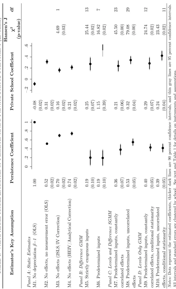
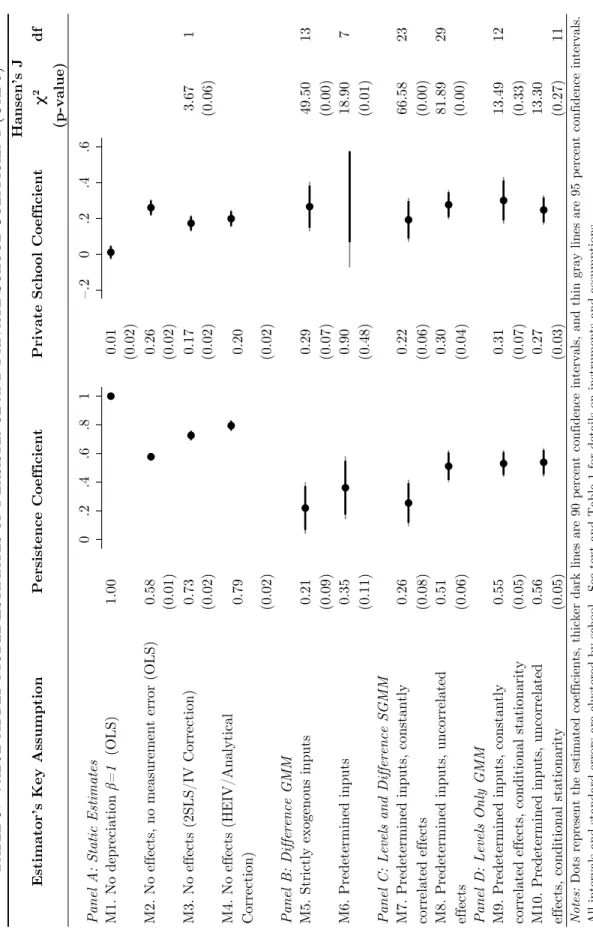
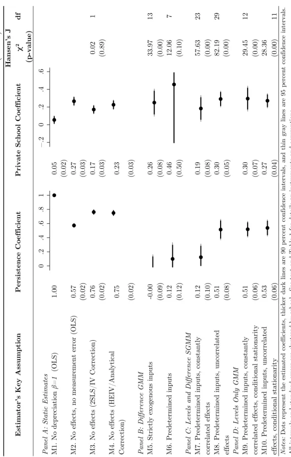
Tables 4 (English), 5 (Urdu), and 6 (mathematics) summarize our main value-added results. All estimates include the full set of controls in the child survey sample, the survey date, round (grade) dummies, and village fixed effects. For brevity, we only report the persistence and
private school coefficients.11 We group the discussion of our results in three domains: estimates
of the persistence coefficient, estimates of the private schooling coefficient, and regression diag-nostics.
4.2.1 The persistence parameter
We immediately reject the hypothesis of perfect persistence (β = 1). Across all specifications
and all subject (except M1 which imposes β = 1), the estimated persistence coefficient is
significantly lower than one, even in the specifications that correct for measurement error only and should be biased upward (M3 and M4). The typical lagged value-added model (M2), which assumes no omitted student heterogeneity and no measurement error, returns estimates between 0.52 and 0.58 for the persistence coefficient. Correcting only for measurement error by instrumenting using the two alternate subjects (M3), or using the analytical correction described by in the appendix (M4), increases the persistence coefficient to between 0.70 and 0.79,
consistent with significant measurement error attenuation. This estimate, however, remains
biased upward by omitted heterogeneity.
Moving to our dynamic panel estimators, Panel B of each table gives the Arellano and Bond (1991) difference GMM estimates under the assumption that inputs are strictly exogenous (M5) or predetermined (M6). In English and Urdu, the persistence parameter falls to between 0.19 and 0.35. The estimates are (statistically) different from models that correct for measurement
error only. In other words, omitted heterogeneity in learning exists, and biases the static
esti-mates upward. For mathematics, the estimated persistence coefficient is indistinguishable from
zero, considerably below all the other estimates. These estimates are higher and somewhat more stable in the systems GMM approach summarized in Panel C (M7, M8).
With the addition of a conditional mean stationarity assumption (Panel D), we can more precisely estimate the persistence coefficient. In this model, we only use moments in levels to illustrate a dynamic panel estimator that improves over the lagged value-added model estimated by OLS but doesn’t require estimating a system of equations. The persistence coefficient rises substantially to between 0.39 and 0.56. This upward movement is consistent with a violation of the stationarity assumption (the fixed-effect still contributes to achievement growth) but an overall reduction in the omitted heterogeneity bias. Across the various dynamic panel models and subjects, estimates of the persistence parameter vary from 0.2 to 0.55. However the highest dynamic panel estimates come from assuming conditional mean stationary, which is likely too strong in the context of education.
11As discussed, time-invariant controls drop out of the differenced models. For the system and levels estimators
we also assume, by necessity, that time-invariant controls are uncorrelated with the fixed effect or act as proxy variables.
4.2.2 The contribution of private schools
Assuming perfect persistence biases the private school coefficient downward. For English, the
estimated private school effect in the restricted model that incorrectly assumesβ = 1(Panel A,
Table 4) is negative and significant. For Urdu and mathematics, the private school coefficient is small and insignificant or marginally significant (Panel A, Tables 5 and 6). By comparison, all the dynamic panel estimates are positive and statistically significant, with the exception of one of the difference GMM estimates, which is too weak to identify the private school effect with any precision.
Panel C (levels and differences GMM) illustrates the benefit of a systems approach. Adding a levels equation (Panel C, Tables 4-6), using the assumption that inputs are constantly correlated or uncorrelated with the omitted effects, reduces the standard errors for the private school coefficient while maintaining the assumption that inputs are predetermined but not strictly exogenous. Under the scenario that private school enrollment is constantly correlated with the omitted effect (M7), the private school coefficient is large: 0.19 to 0.32 standard deviations depending on the subject and statistically significant. This estimate allows for past achievement shocks to affect enrollment decisions but assumes that switching school type is uncorrelated with unobserved student heterogeneity. This is our preferred estimate.
An overarching theme in this analysis is that the persistence parameter influences the esti-mated private school effect but that it is rarely possible to get enough precision to distinguish estimates based on different exogeneity conditions. This is largely due to the small number of children switching between public and private schools in our sample. In Figure 3, we graph the relationship between both coefficients explicitly. Rather than estimating the persistence coefficient, we assume a specific rate and then estimate the value-added model. That is, we
use yit−βyi,t−1 as the dependent variable. This provides a robustness check for any estimated
effects, requires only two years of data, and eliminates the need for complicated measurement error corrections. (It assumes, however, that inputs are uncorrelated with the omitted learning heterogeneity.) As expected given the large baseline differences, the estimated private school effect strongly depends on the assumed persistence rate. Moving from the restricted
value-added model (β = 1) to the pooled cross-section model (β = 0) increases the estimated effect
from negative or insignificant to large and significant. For most of the range of the persistence parameter, the private school effect is positive and significant, but pinning down the precise yearly contribution of private schooling depends on our assumptions about how children learn. A couple of natural questions are how these estimates compare to the private-public dif-ferences reported in the cross-section and why the trajectories in Figure 1 are parallel even though the private school effect is positive. Controlling for observables suggests that after three years, children in private schools are 0.9 (English), 0.5 (Urdu), and 0.45 (mathematics)
stan-dard deviations ahead of their public school counterparts. If persistence is 0.4 and the yearly private school effect is 0.3, children’s trajectories will become parallel when that achievement
gap reaches 0.5 (= 0.3/(1−0.4)). This is roughly the gap we find in Urdu and mathematics.
Any small disagreement, including the larger gap in English, may be attributable to baseline selection effects. Thus our results can consistently explain the large baseline gap in achieve-ment, the parallel achievement trajectories in public and private schools, and the significant and ongoing positive private school effect.
4.2.3 Regression diagnostics
For many of the GMM estimates, Hansen’sJ test rejects the overidentifying restrictions implied
by the model. This is troubling but not entirely unexpected. Different instruments may be identifying different local average treatment effects in the education context. For example, the portion of third grade achievement that remains correlated with fourth grade achievement may decay at a different rate than what was learned most recently. This is particularly true in an optimizing model of skill formation where parents smooth away shocks to achievement. In such a model, unexpected shocks to achievement, beyond measurement error, would fade more quickly than expected gains. Instrumenting using contemporaneous alternate subject scores will therefore more likely identify different parameters than instrumenting using previous year scores. Likewise, instrumenting using alternate lags and differenced achievement and inputs may also identify different effects. This type of heterogeneity is important and suggests that
a richer model than a constant coefficient lagged value-added may be warranted.12 Given the
rejection of the overidentifying restrictions in some cases, the next section provides a series of robustness exercises around the estimation of the persistence parameter.
4.3 Robustness Checks
If our estimates are interpreted as forgetting, children lose over half of their achievement in a single year. For some subjects, such as mathematics, this fraction may be even larger. While the estimates reported may appear to be implausibly high, they match recent work on fade-out in value-added models, as well as the rapid fade-out observed in most educational interventions. Table 7 summarizes six randomized (or quasi-randomized) interventions that followed chil-dren after the program ended. This follow-up enables estimation of both immediate and ex-tended treatment effects. For the interventions summarized, the exex-tended treatment effect represents test scores roughly one year after the particular program ended. For a number of
12Another common strategy to address potentially invalid instruments is to slowly reduce the instrument
set, testing each subset, until the overidentification test is accepted or the model becomes just identified. We explored this approach but no clear story emerged. One result of note is that dropping the overidentifying inputs typically raises the the persistence coefficient slightly, to roughly 0.25 for math.
the interventions, the persistence coefficient is less than 0.10. In two interventions—learning incentives and grade retention—the coefficient is between 0.6 and 0.7. However, this higher
level of persistence may in part be explained by the specific nature of these interventions.13
Although the link between fade-out in experimental studies and the persistence parameter is not always exact, all the evidence suggests that current learning does not carry over to future learning without loss and, in fact, these losses may be substantial.
Exploring the magnitude of thepotential bias in a basic lagged value-added model can also
give us some sense for whether our estimates are reasonable. Consider, for example, the bias in
the regression yit =α+βyi,t−1+ηit, where we have omitted all potential inputs and corrected
only for measurement error bias. Our estimates of this model suggest that the persistence coefficient is at most 0.8 to 0.9—far higher than our highest dynamic panel estimates of around 0.5. Is this discrepancy reasonable?
Aggregating all the omitted contemporaneous inputs into one variableηitimplies the upward
bias of the persistence coefficient isCov(ηit, yi,t−1)/Var(yit−1). If the correlation between inputs
in any two periods is a constant ρX, and all children in grade zero start from the same place,
the persistence coefficient in a lagged value-added model for fourth grade will be biased upward to
Cov(ηi4, yi3)
Var(yi3˙)
= ρX
2βρX −β+β2+ 1. (10)
Figure 4 gives a graphical representation of this bias calculation. To read the graph, choose
a true persistence coefficient, β (the dotted lines), and a degree of correlation of inputs over
time,ρX (the horizontal axis). Given these choices, the y-axis reveals the persistence coefficient
that a lagged value-added specification estimated by OLS would yield. Working with our
estimates, if the true persistence effect, β, is 0.4 and inputs are correlated only 0.6 over time,
the (incorrectly) estimated β will be 0.9. Given that the vast majority of inputs are fixed, this
seems quite reasonable, and perhaps even too low.14
13In the case of grade retention, there is no real “post treatment” period since children always remain one
grade behind after being retained. If one views grade retention as an ongoing multi-period treatment, then lasting effects can be consistent with low persistence. In the case of learning incentives, Kremer, Miguel and Thornton (2003) argue that student incentives increased effort (not just achievement) even after the program ended, leading to ongoing learning.
14Another way to get at the reasonableness of rapid fade out is motivated by Altonji, Elder and Taber’s
(2005) assumption of equal selection on observed and unobserved variables. Absent controls and correcting for
measurement error the persistence coefficient is 0.91, while the R2 of the regression is 0.52. Adding controls
raises theR2only modestly to 0.56 but at the same time reduces the estimated persistence coefficient to 0.74.
Thus, just by explaining an additional four percent of the total variation, we reduced the persistence coefficient substantially. Assuming equal selection on observed and unobserved variables would lead to a persistence
4.4 Why Is Persistence So Low?
The low estimates of persistence are worrying, not only for program evaluation but for the more substantive issue of how to improve cognitive achievement. One major concern is that imperfect persistence is a psychometric testing issue, and therefore not a “true” feature of the learning dynamic. For instance, later test forms may capture fundamentally different latent traits than earlier test forms. To address this concern, we replicated our results using IRT scores based solely on a common set of items that appeared on every test form—our tests had a significant number of overlapping items in each year. Our results were similar using these scores, with the difference GMM persistence estimates in fact dropping slightly. The score equating methods used to create a single cardinal measure of learning therefore do not appear to be the driving force behind the low observed persistence.
Several other possible mechanical explanations for low persistence are also unlikely. First, artificial ceiling effects can appear like low persistence in models that use bounded scores. To address this concern, we exclusively use unbounded IRT scale scores and our exam is designed to maximize the variation over the entire range of observed abilities. Second, cheating, often driven by high stakes testing, can create artificially low estimates of persistence. Jacob and Levitt (2003), for instance, detect teacher cheating in part by looking for poor subsequent performance of students who made rapid gains. In our data, cheating is unlikely both because our test is relatively low stakes and because our project staff administered the exam directly to avoid this possibility. Third, critics of high stakes testing often argue that shallow “teaching to the test” leads to low persistence. This is also an unlikely explanation in our context; our exam is relatively low stakes, is not part of the standard educational infrastructure, and covers only
subject matter that all students should know and that Pakistani parents generally demand.15
We looked at a couple of other candidate explanations, but there are no “smoking guns” that could explain low persistence. Tables 8 and 9, for instance, present the results of a preliminary exercise that assesses whether low persistence arises from household and school re-sponses to unexpected achievement shocks—an explanation that has different implications for
cost-benefit analysis than simple forgetting.16 Parents’ perceptions of their child’s performance
reacts strongly to unexpected gains in achievement, but there is only weak evidence of
substi-15On average, the children tested at the end of Grade 3 could complete two-digit addition, but not subtraction
or multiplication (in mathematics); recognize simple words (but not sentences) in the vernacular (Urdu); and recognize alphabets and match simple three-letter words to pictures in English.
16We examine whether inputs adjust to unexpected achievement shocks for roughly 650 children for whom we
have detailed information from a survey collected at households. As a measure of the unexpected shock, we first compute the residual from a regression of fourth grade scores on third grade scores and a host of known controls. We then test whether this residual predicts changes between fourth and fifth grade in parents’ perceptions of the child’s performance, expenditure on school, and time spent helping children on homework, being tutored, doing homework, and playing.We instrument for the subject specific residuals using the alternate subject residuals to lessen measurement error attenuation.
tution effects. School expenditures do drop slightly as do the hours spent helping the child on his or her homework. Minutes spent playing increases, but tuition also increases. While some of these responses are in the direction of substitution, they are generally not statistically signif-icant. Given the detailed household data we obtained, it suggests that household substitution is unlikely to be a main driver behind low persistence. This may not be particularly surprising given that very low achievement suggests that children may be below parents’ desired learning levels.
Table 9 explores the possibility that fade out captures teachers targeting poorly performing students. If teachers target poorly performing children in each classroom, persistence should be lower within schools than between schools. To test this hypothesis, we estimate a basic lagged value-added model with no controls and instrument for lagged achievement using lagged differences in alternate subjects. We estimate this model using average school scores (between school specification) and child scores measured in deviations for the school average (within school specification). If anything, the persistence coefficient is lower for the between school regressions, suggesting that within school targeting is not the primary reason for low persistence. Finally, Table 10 looks at whether heterogeneity in persistence can provide some hints about
its origin(Semb and Ellis, 1994).17 To obtain the most power possible, we estimate the
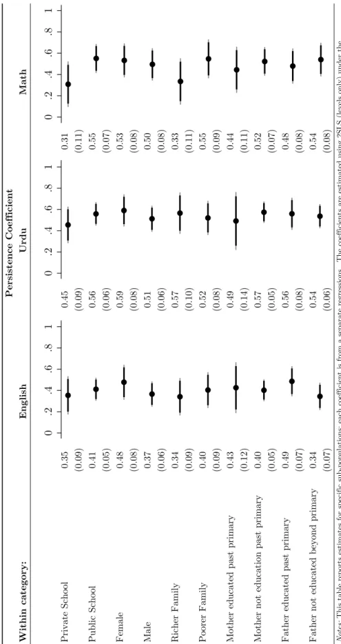
value-added model for specific sub-populations using the “predetermined inputs, uncorrelated effects, and conditionally stationary” based estimator (M10 of Tables 4, 5, and 6). Unfortunately, large standard errors make it difficult to find statistically different decay rates between groups. Learning in private schools seems to decay faster than learning in government schools, but the difference is not statistically significant. A similar pattern holds for richer families and children with educated parents. These results hint that learning decays faster for faster learners.
These candidate explanations do not yield a compelling story thus far; it could just be that children forget what they learned. Psychology and neuroscience provide some compelling evi-dence for this using laboratory experiments. Psychological research on the “curve of forgetting” dates back to Ebbinghaus’s (1885) seminal study on memorization. Rubin and Wenzel (1996) review the laboratory research spawned by this contribution. Semb and Ellis (1994) review classroom studies that test how much students remember after taking a course. Both litera-tures document the fragility of human memory. Cooper et al. (1996) studies the learning losses that children experience between spring and fall achievement tests. These losses are generally not as rapid as the effects we find, but the experiment is different: we estimate the depreciation with no inputs, whereas summer activities provide some stimulus, particularly for privileged
17To give one example, MacKenzie and White (1982) report that fade out for geographical knowledge was
much higher for in-class exercises compared to field excursions (or, passive versus active learning.) Similarly, Rothstein (2008) finds heterogeneity in the long-run effects of teachers who produce equal short-run gains; Jacob, Lefgren and Sims (2008) estimate that teacher effects are only a third as persistent as achievement in general.
children.
5 Conclusion
In the absence of randomized studies, the value-added approach to estimating education pro-duction functions has gained momentum as a valid methodology for removing unobserved indi-vidual heterogeneity in assessing the contribution of specific programs or in understanding the contribution of school-level factors for learning (e.g. Boardman and Murnane, 1979; Hanushek, 1979; Todd and Wolpin, 2003; Hanushek, 2003; Doran and Izumi, 2004; McCaffrey, 2004; Gor-don, Kane and Staiger, 2006). In such models, assumptions about learning persistence and unobserved heterogeneity play central roles. Our results reject both the assumption of perfect persistence required for the restricted value-added model and of no learning heterogeneity re-quired for the lagged value-added model. Our results for Pakistan should illustrate the danger of incorrectly modeling or estimating education production functions: the restricted value-added model is fundamentally misspecified and can even yield wrong-signed estimates of a program’s impact. Underscoring the potential of affordable, mainstream, private schools in developing countries, we find that Pakistan’s private schools contribute roughly 0.25 standard deviations more to achievement each year than government schools, an effect greater than the average yearly gain between third and fourth grade.
Our estimate of persistence is consistent with recent work on teacher effects, with analytical and empirical estimates of the expected bias under OLS, and with experimental evidence of program fade out in developing and developed countries. But the economic interpretation still remains an open area of enquiry. Our context and test largely rule out mechanical explanations of low persistence. We also find little evidence that low persistence results from substitution by parents and teachers; the behavioral adjustments we are able to measure are unlikely to represent the primary reason achievement gains fade out. Simple forgetting, consistent with a large body of memory research in psychology, appears to be a likely explanation and hence a core component of education production functions, although more research is needed to provide direct evidence for it.
Our results also highlight that short evaluations, even when experimental, may yield little information about the cost-effectiveness of a program. Using the one or two year increase from a program gives an upper-bound on the longer term achievement gains. As our estimates suggest, and Table 7 confirms, we should expect program impacts to fade quickly. Calculating the internal rate of return by citing research linking test scores to earnings of young adults is therefore a doubtful proposition. The techniques described here, with three periods of data, can theoretically obtain a lower bound on cost-effectiveness by assuming exponential fade out. At the same time, the causes of fade out are equally important: if parents no longer need to hire
tutors or buy textbooks (the substitution interpretation of imperfect persistence), a program
may be cost-effective even if test scores fade out.
Moving forward, empirical estimates of education production functions may benefit from further unpacking persistence. Overall, the agenda pleads for a richer model of education and for empirical techniques for modelling the broader learning process, not simply to add nuance to our understanding of learning, but to get the most basic parameters right.
A Analytical Corrections for Measurement Error
Consider the lagged value-added model
yit∗ =α#xit+βyi,t∗ −1+vit, (11)
where y∗it and yi,t∗ −1 are true achievement, vit is the error term, and we have put aside the
possibility of omitted heterogeneity. Since achievement is a latent variable, we can only estimate it with error. Thus, we actually estimate
yit=α#xit+βyi,t−1+ [vit+εit−βεi,t−1] (12)
and OLS is inconsistent because yi,t−1 is correlated with εi,t−1.
The analytic correction we apply replacesyi,t−1 with the best linear predictor
˜
yi,t−1 ≡E∗[yi,t∗ −1 |yi,t−1,xit] =λ#xit+ri,t−1yi,t−1, (13)
where λ and ri,t−1 are parameters. To see why this works, add and subtract βyi,t˜ −1 from (11)
to get
yit=xitα+βy˜i,t−1+ [β(yi,t−1−y˜i,t−1) +vit+εit−βεit−1] (14)
=xitα+βyi,t˜ −1+ [β(yi,t∗ −1−yi,t˜ −1) +vit+εit]. (15)
where the second line follows from y∗
i,t−1 =yi,t−1−εit−1. Assuming exogeneity with respect to
vit+εit, OLS is consistent if
E[x#it(yi,t∗ −1−yi,t˜ −1)] = 0, (16)
E[˜yi,t−1(yi,t∗ −1−yi,t˜ −1)] = 0. (17)
These conditions are automatically satisfied since the fitted value yi,t˜ −1 and independent
vari-ables xit are orthogonal to the residual yi,t∗ −1−yi,t˜ −1 by the definition of the projection (13).
The only difficulty is estimating the projection parametersλ andri,t−1 since the dependent
variable y∗
i,t−1 is unobserved. But it turns out that we do not need to observe the true score.
The orthogonality conditions that define the projection (13) are
E[x#it(yi,t∗ −1−λ#xit−ri,t−1yi,t−1)] = 0, (18)
E[y#i,t−1(yi,t∗ −1−λ#xit−ri,t−1yi,t−1)] = 0. (19)
Solving first for λ, we have
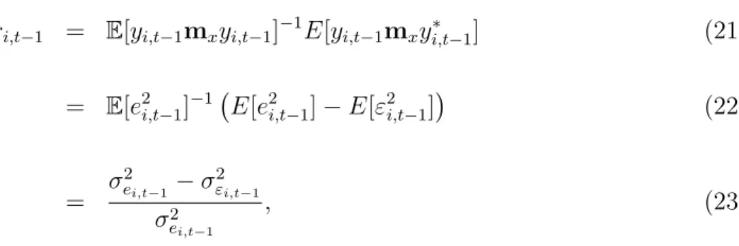
Plugging (20) into (19) and solving for ri,t−1 yields
ri,t−1 = E[yi,t−1mxyi,t−1]−1E[yi,t−1mxyi,t∗−1] (21)
= E[e2i,t−1]−1$E[e2i,t−1]−E[ε2i,t−1]% (22)
= σ 2 ei,t−1 −σ 2 εi,t−1 σ2 ei,t−1 , (23)
where mx ≡1− xit(x#itxit)−1x#it is an annihilator vector andei,t−1 is the residual from a
regres-sion of yi,t−1 on xit. We can estimate ri,t−1 by computing σ2ei,t−1 from the regression of yi,t−1
on xit and taking σε2i,t−1 from IRT—i.e., from the inverse Fisher information matrix of θˆ.
In-tuitively, ri,t−1 is the heteroscedastic reliability ratio of the score minus the variation explained
by the independent variables. That is, the reliability ratio ofyi,t−1−E[y∗i,t−1 |xit].
We computeλ by plugging ri,t−1 into (20) to get
λ = E[x#itxit]−1E[xit# (y∗i,t−1−ri,t−1yi,t−1)] (24)
= E[x#itxit]−1E[x#ityi,t−1](1−ri,t−1). (25)
The best predictor is ˜
yi,t−1 =E[yi,t−1|xit](1−ri,t−1) +ri,t−1yi,t−1 (26)
This takes the familiar form of an empirical Bayes estimate that shrinks the observed score to the predicted mean. The shrinkage performs the same function as blowing up the coefficient using the reliability ratio after estimation. Here, however, our shrunken estimate provides a more efficient correction by using the full heteroscedastic error structure (Sullivan, 2001) .
Table A1 reports persistence coefficients corrected only for measurement error using the instrumental variable (using alternate subjects) and the analytical correction approach. Each cell contains the estimated coefficient on lagged achievement from a regression with no controls and the associated standard error. Where applicable, we also report the p-value for Hansen’s overidentification test statistic. This is possible for the instrumental variables estimators since we have three subject tests and three years of data.
Absent any correction (OLS), the estimated persistence coefficient ranges between 0.65 and 0.70. Instrumenting using alternate subjects raises the estimated coefficient significantly to 0.85 for English, 0.89 for mathematics, and 0.97 for Urdu. However, the overidentifying restriction is rejected at the one percent level in all three subjects. This suggests that measurement errors may be correlated across subjects at the same sitting and that this correlation may differ depending on the subject. By comparison, when we instrument for lagged achievement using double lagged scores we cannot reject the overidentifying restrictions. Unfortunately, in the context of dynamic panel methods, additional lags to address measurement error require
T = 4. The final line of Table A1 shows estimates based on our analytical correction around