Integrated hydro-bacterial modelling for predicting bathing water quality Guoxian Huang, Roger A. Falconer, Binliang Lin
PII: S0272-7714(16)30382-1 DOI: 10.1016/j.ecss.2017.01.018 Reference: YECSS 5395
To appear in: Estuarine, Coastal and Shelf Science
Received Date: 21 September 2016 Revised Date: 12 January 2017 Accepted Date: 13 January 2017
Please cite this article as: Huang, G., Falconer, R.A., Lin, B., Integrated hydro-bacterial modelling for predicting bathing water quality, Estuarine, Coastal and Shelf Science (2017), doi: 10.1016/ j.ecss.2017.01.018.
This is a PDF file of an unedited manuscript that has been accepted for publication. As a service to our customers we are providing this early version of the manuscript. The manuscript will undergo copyediting, typesetting, and review of the resulting proof before it is published in its final form. Please note that during the production process errors may be discovered which could affect the content, and all legal disclaimers that apply to the journal pertain.
M
AN
US
CR
IP
T
AC
CE
PT
ED
1Integrated Hydro-bacterial Modelling for Predicting
1
Bathing Water Quality
2
Guoxian Huang1,2, Roger A. Falconer1,* and Binliang Lin1,2 3
1
Hydro-environmental Research Centre, School of Engineering, Cardiff University, 4
Cardiff, CF24 3AA, UK; 5
E-Mails: [email protected]; (G.H.); [email protected] (B.L.) 6
2
Department of Hydraulic Engineering, Tsinghua University, Beijing 100084, 7
China 8
* Author to whom correspondence should be addressed: 9
Email:[email protected] 10
Tel.: +44-292-087-4280. 11
Abstract: In recent years health risks associated with the non-compliance of bathing 12
water quality have received increasing worldwide attention. However, it is 13
particularly challenging to establish the source of any non-compliance, due to the 14
complex nature of the source of faecal indicator organisms, and the fate and delivery 15
processes and scarcity of field measured data in many catchments and estuaries. In 16
the current study an integrated hydro-bacterial model, linking a catchment, 1-D 17
model and 2-D model were integrated to simulate the adsorption-desorption 18
processes of faecal bacteria to and from sediment particles in river, estuarine and 19
coastal waters, respectively. The model was then validated using hydrodynamic, 20
sediment and faecal bacteria concentration data, measured in 2012, in the Ribble 21
river and estuary, and along the Fylde coast, UK. Particular emphasis has been 22
M
AN
US
CR
IP
T
AC
CE
PT
ED
2placed on the mechanism of faecal bacteria transport and decay through the 1
deposition and resuspension of suspended sediments. The results showed that by 2
coupling the E.coli concentration with the sediment transport processes, the accuracy 3
of the predicted E.coli levels was improved. A series of scenario runs were then 4
carried out to investigate the impacts of different management scenarios on the E.coli 5
concentration levels in the coastal bathing water sites around Liverpool Bay, UK. 6
The model results show that the level of compliance with the new EU bathing water 7
standards can be improved significantly by extending outfalls and/or reducing urban 8
sources by typically 50%. 9
Key words: Cloud to Coast (C2C); Computational Hydraulics; Faecal Indicator 10
Organisms; Health Impact Assessment; Sediment Transport, Water quality. 11
1. Introduction 12
Bathing water quality is of increasing international concern, and public 13
awareness of the impacts of poor bathing water quality on health risk has increased 14
in recent years. Beach closures now frequently occur due to the non-compliance of 15
water quality to the required standards. It is therefore increasingly a challenge to 16
balance wastewater disposal with other activities in estuarine and coastal waters 17
(Bedri et al., 2016). In order to comply with the standards required by regulatory 18
authorities world-wide, many bathing water quality improvement measures have 19
been drawn up and many projects have been carried out worldwide to study non-20
compliance. For example: the TIMOTHY project in Belgium (de Brauwere et al., 21
2011; Ouattara et al., 2013), the Southern California Coastal Water Research Project 22
(de Brauwere et al., 2014a; Field and Samadpour, 2007; Griffith et al., 2009) and 23
Michigan Lake (Liu et al., 2013; Pramod et al., 2010; Safaie et al., 2016) in the USA, 24
M
AN
US
CR
IP
T
AC
CE
PT
ED
3Hong Kong, China (Chan et al., 2013; Thoe et al., 2012) and the Cloud to Coast 1
project (C2C) in the UK (http://www.shef.ac.uk/c2c/index), are all examples of 2
studies undertaken to investigate bathing water quality. However, bathing water non-3
compliance is a complex problem, since it involves many aspects and processes 4
(Huang et al., 2015b) including: catchment management (Byappanahalli et al., 2015), 5
arrangements relating to the siting of sewage pipe networks and outfalls (Fan et al., 6
2015; Obiri‐Danso and Jones, 1999), waste water treatment methods, weather
7
conditions (Ackerman and Weisberg, 2003; Kashefipour et al., 2002), sediment 8
suspension and transport (Gao et al., 2013), currents, waves, and sea birds and pets 9
(Converse et al., 2012; Wither et al., 2005; Wright et al., 2009) etc. Moreover, it is 10
still unfeasible to track the sources of Faecal Indicator Organisms (FIOs) and predict 11
the fate and transport of FIO processes (Boehm et al., 2002), based only on case-12
specific measured data with a low spatio-temporal resolution (de Brauwere et al., 13
2014b). 14
Many hydrological models have been developed to predict the hydrological and 15
FIO transport process in river catchments, e.g. the semi-distributed model Soil and 16
Water Assessment Tool (SWAT) (Arnold and Fohrer, 2005; Cho et al., 2012), the 17
Hydrological Simulation Program—FORTRAN (HSPF) (Benham et al., 2006; Liao 18
et al., 2015) and the distributed model (Huang et al., 2015b; Niu and Phanikumar, 19
2015). Hydrodynamic and water quality models have been developed for bacteria 20
process predictions in river networks (Yakirevich et al., 2013; Yang et al., 2002) and 21
estuaries (Gao et al., 2013; Liao et al., 2015; Thupaki et al., 2013). Numerical model 22
studies have also been undertaken for predicting FIO processes in both rivers and 23
coastal waters (de Brauwere et al., 2014a; Huang et al., 2015a), and in some cases a 24
catchment model is used to supply the upper boundary conditions (Bedri et al., 25
M
AN
US
CR
IP
T
AC
CE
PT
ED
42014; Huang et al., 2015b). To summarize, these numerical models can be used (de 1
Brauwere et al., 2014b) to: (i) identify the sources, processes and parameters 2
controlling FIO dynamics; (ii) assess the impacts of natural events and human 3
activity on bathing water quality; and (iii) support real-time decision making by 4
providing short-term predictions of FIO distributions at bathing water and shellfish-5
harvesting sites. 6
Since the complex processes of the source, transport and fate of FIOs can occur 7
in the catchments, sewage works, riverine and estuarine waters, and they are closely 8
linked with environmental and sedimentary factors, it is difficult to use existing 9
numerical models to reproduce the FIO processes for the whole study area, i.e from 10
Cloud to Coast. At present, quantitative evaluation of bathing water improvements 11
by various measures still involve significant uncertainties. Therefore, the main 12
objective of this study has been to develop an integrated hydro-bacterial modelling 13
system to quantify more accurately the effects of bathing water improvement 14
measures on the water quality characteristics and particularly in terms of the FIO 15
levels. The system comprises: two hydrological models, a 1-D river and sewage pipe 16
network model and the 2-D/3-D Environmental Fluid Dynamics Code (EFDC) 17
model. These models have been integrated to predict the fate and transport processes 18
of FIOs from the upstream catchments, through pipe network and/or river systems to 19
the estuarine and coastal waters. The FIO fluxes have been linked to the sediment 20
transport processes, which are considered to be important in order to improve on the 21
model predictive accuracy of FIO levels in river and estuarine waters. The model 22
was first validated using hydrodynamic data and then further validated using 23
sediment and faecal bacteria concentration data, measured in the river Ribble and its 24
estuary in 1999 and 2012. In this study, E.coli has been used as the representative 25
M
AN
US
CR
IP
T
AC
CE
PT
ED
5indicator for FIOs. A series of scenario runs have also been carried out to investigate 1
the most efficient management strategy for reducing E.coli concentration levels 2
along the bathing water beaches around the Ribble Estuary and Fylde Coast. 3
2. Materials and methods 4
2.1 Outline of the Integrated Model 5
The integrated modelling system is composed of 5 sub-models and a brief 6
description of the system and the linkage between the sub-models is given below. 7
(1) HSPF model
8
The Hydrological Simulation Program – FORTRAN (HSPF) (Bicknell et al., 9
1997) is a sophisticated and comprehensive watershed model that simulates runoff 10
and diffuse (or non-point) pollutant loads, for various land cover configurations and 11
enables the fate and transport processes of solutes to be predicted in streams. HSPF 12
comprises three main modules, including: PERLND, IMPLND, and RCHRES, and 13
five auxiliary modules. In HSPF, the watershed is represented in terms of land 14
segments and stream reaches. The PERLND module is used to simulate the 15
hydrological and water quality processes over pervious areas, while IMPLND is used 16
for impervious land, where infiltration is very small and can be omitted. Compared 17
with distributed hydrological models with grid cells, HSPF has a high computational 18
efficiency with reasonable accuracy. 19
(2) Infoworks model
20
The Infoworks model includes a distributed rainfall-runoff model and a pipe 21
network model, built and simulated using the Infoworks CS software package. It can 22
M
AN
US
CR
IP
T
AC
CE
PT
ED
6be used to solve the hydrological, hydrodynamic and water quality processes in 1
urban catchments, rivers, drainage and sewerage networks and related devices. A 2
more detailed description of the urban model is given in the Hydroworks/Infoworks 3
CS menu (Wallingford Software Ltd, 1995) and various papers, such as (Rico-4
Ramirez et al., 2015) Rico-Ramirez et al. (2015).. 5
(3) DMHSF model
6
A distributed catchment model (Huang et al., 2015b), which has been developed 7
to simulate the hydrological, sediment transport and faecal indicator organism 8
processes in river basin catchments, is based on the Xinanjiang (XAJ) flow yield 9
mechanism (Zhao, 1992). In this model, the E.coli transport processes are associated 10
with sediment transport fluxes, with the decay rate for E.coli being dependent upon 11
temperature and irradiance, and with the E.coli being adsorbed or desorbed onto or 12
from the sediment particles. 13
(4) One-dimensional river network model (RMN1D)
14
A one-dimensional river network model has been developed to predict the 15
hydrodynamic and water quality processes in riverine basins. The model has been 16
applied to the complex network of rivers associated with the Ribble basin. In this 17
model, the implicit four point Pressimann finite difference scheme has been used for 18
the hydrodynamic solution (Huang et al., 2016). Meanwhile, the finite volume 19
method, with a staggered grid, has been used to improve on mass conservation for 20
the sediment and water quality flux predictions. The model has proven to be highly 21
accurate for simulating solute concentration levels in river networks, such as the 22
M
AN
US
CR
IP
T
AC
CE
PT
ED
7Ribble, and particularly for E.coli concentration values which can vary from near 1
zero to many millions. 2
(5) Modified EFDC 2D/3D model 3
The Environmental Fluid Dynamics Code (EFDC) is a general purpose 4
modelling package developed at the Virginia Institute of Marine Science for 5
simulating hydrodynamic, solute and biogeochemical processes in surface water 6
systems (Hamrick, 1992). The model deploys a curvilinear-orthogonal co-ordinate 7
system in the horizontal direction and a stretched sigma coordinate system in the 8
vertical direction. It uses a finite volume-finite difference spatial discretization, with 9
a staggered grid, to solve the governing equations representing the hydrodynamic, 10
water-quality and sediment transport processes. A second moment turbulence closure 11
model, developed by Mellor and Yamada (1982) and modified by Galperin et al. 12
(1988), is used to provide the vertical turbulent viscosity and diffusivity. This 13
turbulence closure model relates the vertical turbulent viscosity and diffusivity to the 14
turbulence intensity and length scales. The EFDC model is second-order accurate in 15
both space and time and is well documented and widely used. 16
2.2 Model Verification 17
2.2.1 Site Description 18
The model domain covered part of North West England, with about 9660 km2 and
19
12920 km2 for the coastal region and catchments respectively (see Figure 1a). The bed
20
elevation ranged from -60 m to 866 m, and the minimum and maximum elevation 21
regions were mainly located to the western edge of the sea boundary and the source 22
regions of rivers Dee, Mersey and Lune, respectively. There were 11 main rivers 23
included in the model, flowing into the coastal region along the East and North banks. 24
M
AN
US
CR
IP
T
AC
CE
PT
ED
8In the extensively wide transitional lowland zones between the mountains and 1
estuaries, major cities, such as Manchester, Preston, Liverpool, Blackpool, Chester are 2
located at the lower and middle reaches of these rivers or around the main bay. 3
Meanwhile, there are extensive arable and improved grass lands for crops and 4
livestock breeding around these cities, which needed to be included in the catchment 5
models. The well-known bathing water sites of Blackpool and Lytham St Annes are 6
located between the deltas of rivers Wyre and Ribble, including the river Ribble 7
network and its estuary. The domain was located along the North West region of 8
England, with a total basin area of 1583 km2. The river Ribble rises in the Yorkshire
9
Pennines and has a length of around 75 miles in main channel length, with 3 key 10
tributaries, including: the Hodder, Calder and Darwen. 11
The hydrological and hydrodynamic computational sub-domains were extended to 12
the other adjacent regions, especially considering the intense mixing due to the strong 13
currents and related matter transport, partly associated with the bathymetry. In recent 14
decades, non-compliance of bathing water quality has frequently occurred for the 15
bathing beaches around the Ribble delta, although there has been a significant 16
improvement in recent years due to the construction of a series of infrastructure assets, 17
which have improved the water quality in the region. 18
M
AN
US
CR
IP
T
AC
CE
PT
ED
9 UK 10000 m ( (( (a)))) (b)Figure 1. (a) Map of the study area including: monitoring sites and bathing 1
water compliance sites for the rivers and coastal region; and (b) view of the 2
nearshore region around the Ribble estuary, showing the original outfall 3
locations and extended locations, together with planned outfalls. 4
2.2.2 Model Set-up 5
In modelling the Ribble catchment, the hydrological and E.coli simulation in the 6
rural catchments were carried out by the c2c participants from Sheffield University 7
(Phillips, 2014) using the HSPF model, where 52 sub-catchments with an average of 8
10 segments were used in the sub-catchments. If sewage pipe networks were also 9
involved, then the Infoworks model which is built by Shepherd (2015) was used to 10
simulate the hydrodynamic and E.coli processes in these pipe networks and the 11
related outputs were then included in the HSPF model as point sources. Meanwhile, 12
the hydrological and E.coli processes in the catchments were calculated by a 13
2000 m
Origenal outfalls
SourthPort Fleetwood Chartworth 1&2
Manchester Square Chartworth Anchorsholme Harrowside Fairhaven Extended outfalls Outfalls (by UU)
M
AN
US
CR
IP
T
AC
CE
PT
ED
10distributed hydrological model system (Huang et al., 2015b), except for the river 1
Ribble and sediment concentrations in the catchment domain. The curvilinear grid 2
was refined to give a higher resolution near the bathing water sites and the river delta 3
regions (see Figure 1b). The bathymetry, bed sediment size distribution, bed 4
roughness values, and the initial and boundary conditions were setup using the EFDC 5
model, including the coastal region and the river network inputs (Huang et al., 2015a). 6
The rivers Ribble, Wyre, Mersey and Lune were all modelled up to the tidal limits 7
in the estuaries, using the EFDC 2D model, while the middle and upstream reaches of 8
the river Ribble were modelled using RNM-1D. The main channels were included as 9
they were located relatively close to the region of interest, i.e. the bathing water sites 10
along the Fylde Coast and the Ribble Estuary. For the key focused coastal domain, the 11
boundary conditions at the open seaward boundary were specified based on the tidal 12
level data obtained using the EFDC-2D hydrodynamic model for the Irish Sea region 13
(Zhou et al., 2014). A constant salinity level of 35 ppt, a temperature value of 20.0oC,
14
a suspended sediment concentration of 5 mg/l and an E.coli concentration of 10 15
cfu/100ml were all assumed at the seaward boundary. At the upper riverine 16
boundaries the measured data acquired in 1999 (Kashefipour et al., 2002) and the 17
modelling data acquired in 2012 from the 1-D and HSPF or distributed catchment 18
models(Huang et al., 2015b) were specified respectively. The inputs included: 19
discharges, suspended sediment and E.coli concentration data, and a water 20
temperature time series, obtained from the UK Meteorological Office. Lateral point 21
sources were also included using either measured data for 1999 or predicted using the 22
catchment models for 2012. 23
M
AN
US
CR
IP
T
AC
CE
PT
ED
112.2.3 Linkage of different models and calculation efficiency 1
In considering the large differences in the time step, calculation speed, and model 2
formats for the different types of land use considered, a simple data flow and model 3
linkage procedure was used in the model system. For the river Ribble catchment the 4
outflow results obtained from the HSPF and Infoworks models were used to provide 5
the upper and lateral boundary conditions to the RNM1D model. For other catchments, 6
where the sewage network data were unavailable, the DMHSF model was used to 7
simulate the flow, sediment and E.coli processes, with the related processes in the 8
sewage pipes being simplified to some degree. Finally, all of the output data from the 9
1D model and parts of the catchment model output data were inputted into the EFDC-10
2D model to predict the sediment and FIO concentrations in the estuarine and coastal 11
waters. Because the upper boundaries of the 2D model were located in the region of 12
the tidal limit, any calculation errors in the hydrodynamic and mass transport 13
predictions would be relatively small. 14
A personal computer with a speed of 3.4 GHz was used throughout this study; it 15
took about 100 hours to undertake one month of simulations of the hydrodynamic, 16
sediment and FIO processes for the whole study area. In the model system, the 17
calculation efficiency was mainly governed by the EFDC 2D model due to its large 18
model domain and the fine grid structure in the estuarine and coastal areas. The 19
catchment and 1D models took much less computational time. 20
2.2.4 Hydrodynamic Verification 21
Comparisons were made between the model predicted water level and velocity 22
values and their corresponding field measurements, at selected sites in the Ribble 23
Estuary, Morecambe Bay, Liverpool Bay and other key sites. The water levels 24
M
AN
US
CR
IP
T
AC
CE
PT
ED
12predicted by the model generally agreed well with the field measurements, with an 1
example prediction being shown in Figure 2, at station L5 near Blackpool. For the 2
comparisons between the field observed and model predicted velocities, some 3
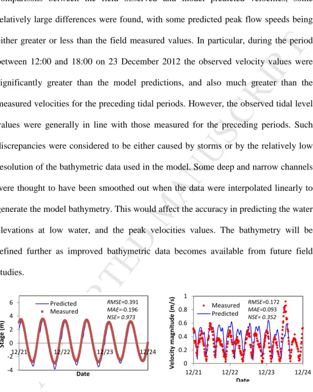
relatively large differences were found, with some predicted peak flow speeds being 4
either greater or less than the field measured values. In particular, during the period 5
between 12:00 and 18:00 on 23 December 2012 the observed velocity values were 6
significantly greater than the model predictions, and also much greater than the 7
measured velocities for the preceding tidal periods. However, the observed tidal level 8
values were generally in line with those measured for the preceding periods. Such 9
discrepancies were considered to be either caused by storms or by the relatively low 10
resolution of the bathymetric data used in the model. Some deep and narrow channels 11
were thought to have been smoothed out when the data were interpolated linearly to 12
generate the model bathymetry. This would affect the accuracy in predicting the water 13
elevations at low water, and the peak velocities values. The bathymetry will be 14
refined further as improved bathymetric data becomes available from future field 15
studies. 16
(a) Water level (b) Velocity
Figure 2. Verification of water level and velocity predictions at a typical coastal 17
monitoring site L5 in 2012, as shown in Figure 1b. 18 -4 -2 0 2 4 6 12/21 12/22 12/23 12/24 S ta g e ( m ) Date Predicted Measured RMSE=0.391 MAE=-0.196 NSE= 0.973 0 0.2 0.4 0.6 0.8 1 12/21 12/22 12/23 12/24 V e lo ci ty m a g n it u d e ( m /s ) Date Measured Predicted RMSE=0.172 MAE=0.093 NSE= 0.352
M
AN
US
CR
IP
T
AC
CE
PT
ED
13 2.2.5 Sediment Verification 1The numerical model results showed that the relatively high suspended sediment 2
concentrations (SSCs), ranging from 100 to 300 mg/l, appeared in the estuarine and 3
shallow coastal regions. The sediments were predicted to have originated from the 4
main feeding rivers, transported by the riverine flows and tidal currents from the 5
rivers to the estuarine and coastal waters. Subsequently, the periodic SSC fluctuations 6
were caused by regional erosion and resuspension, induced by the tidal currents. At 7
the bathing sites, i.e. primarily at Blackpool and Lytham St Annes, the SSCs were 8
found to be lower than the corresponding SSCs in the delta regions. The sediments 9
were thought to be transported from Morecambe Bay, the Wyre and Ribble deltas 10
through the complex sediment-laden currents. This was due to the relatively large 11
proportion of coarse and fine sands along the beaches and the long distance from the 12
river delta to the source. Meanwhile, the FIOs adsorbed on the sediments, have been 13
transported with the sediments from the rivers Ribble and Wyre and have been 14
deposited along the bathing beaches following certain specific hydrodynamic 15
conditions. The predicted and measured comparisons for SSCs are shown for two 16
typical sites, namely No. 713019 and MP11 in the Ribble main channel and estuary, 17
respectively (see Figures 3). 18
(a) No. 713019 in River Ribble (b) No. MP11 in Ribble Delta
0 40 80 120 07/10 07/30 08/19 09/08 S S C (m g /l ) Date 713019 Measured Predicted RMSE=17.7 MAE=-1.55 NSCE= 0.57 0 100 200 300 400 06/03 06/04 06/05 S S C ( m g /l ) Date MP11 Measured Predicted RMSE=77.7 ME=41.30 NSCE= 0.62
M
AN
US
CR
IP
T
AC
CE
PT
ED
14Figure 3. Suspended Sediment Concentration (SSC) verification at two typical 1
monitoring sites. 2
The numerical model predicted SSCs showed encouraging agreement with the 3
corresponding measured data at all sites. For example, in the upper reaches of the 4
river basin (i.e. Figure 3a), the highly episodic variations in the SSCs were generally 5
well reproduced using the distributed hydrological model. Likewise, in the estuary at 6
Milepost 11 (i.e. Figure 3b), the more slowly varying SSCs were also well predicted 7
using by the EFDC-2D model. The SSC distributions around the whole Fylde Coast 8
are also shown at low and high tide respectively in Figure 4. The results show 9
relatively high concentration levels across much of Morecambe Bay, to the north, and 10
in the Ribble Estuary, with the levels in the latter being noticeably higher for low, vis-11
à-vis high, tides. It was found that the suspended sediment fluxes from Morecambe 12
Bay, and the rivers Mersey, Ribble and Wyre governed the SSC distribution across 13
the domain. Local erosion and deposition near Blackpool North may also have had 14
some effect. The main sediment deposition area was identified as being around the 15
river deltas of the Ribble and Wyre and with the relatively low tidal currents in the 16
region of Blackpool therefore providing good conditions for safe bathing. 17
M
AN
US
CR
IP
T
AC
CE
PT
ED
15(a) Low water
(b) High water
Figure 4. Suspended sediment concentration distributions at: (a) low, and (b) high 1
spring tide on 6th August, 2012 2
2.2.6 Faecal Indicator Organism (FIO) Calibration and Tests 3 (1)Model calibration 4 x(m) y (m ) 300000 350000 400000 380000 400000 420000 440000 460000 480000 360 340 320 300 280 260 240 220 200 180 160 140 120 100 80 60 40 20 0 Tidal level: m Wind Mag: m/s SSC (mg/l) Date: 0 5 10 15 20 25 30 Wind Dir: Radiation Watts/m^2 Rainfall: mm/hr Total inflow m^3/s Ribble Inflow: m^3/s Humidity: % Temperature Deg. Cloud: Fractional 6.0 4.0 2.0 0.0 -2.0 -4.0 -6.0 Time(d) T id a l le v e l (m ) 05 0 05 5 0 60 07 0 075 080090 100 120 130 150 180 190 210 230 250 260 280 300 310 326355 420 430 440 450459 2012-08-06 07:30:00 2.91 638. 0.8 0.0 91.3 11.4 482.8 38.9 -3.7 x(m) y (m ) 300000 350000 400000 380000 400000 420000 440000 460000 480000 360 340 320 300 280 260 240 220 200 180 160 140 120 100 80 60 40 20 0 Tidal level: m Wind Mag: m/s SSC (mg/l) Date: 0 5 10 15 20 25 30 Wind Dir: Radiation Watts/m^2 Rainfall: mm/hr Total inflow m^3/s Ribble Inflow: m^3/s Humidity: % Temperature Deg. Cloud: Fractional 6.0 4.0 2.0 0.0 -2.0 -4.0 -6.0 Time(d) T id a l le v e l (m ) 05 0 05 5 06 0 07 0 0 75 080090 100 120 130 150 180 190 210 230 250 260 280 300 310 326355 420 430 440 450459 2012-08-06 13:30:00 2.65 1474. 0.7 0.0 79.2 13.2 428.2 37.3 3.2
M
AN
US
CR
IP
T
AC
CE
PT
ED
16In order to predict the E.coli concentration distributions as accurately as possible, 1
the decay rate was represented dynamically and expressed in the form of T90 values,
2
i.e. the time specified in hours for the concentration to reduce by 90%. Based on 3
recent data acquired by the Centre for Research into Environment and Health 4
(CREH), at Aberystwyth University (http://www.shef.ac.uk/c2c/dissemination/ 5
events), which are presented in table 1, with the T90 values in the modelling system 6
being based on a simplified for day and night variation only. In addition, since E.coli 7
in the river and marine bed material can survive up to 1-2 months (Davies et al., 1995; 8
Garzio-Hadzick et al., 2010)-2 , T90 in the bed sediments was therefore et to 30d in 9
the modelling system. The corresponding T90 value was then converted to an
10
equivalent decay rate kd (with units of sec-1), and with this decay rate being corrected 11
according to the local water temperature. The E.coli concentrations were then coupled 12
to the suspended sediment concentrations, to take into account the effects of 13
adsorption and desorption of the bacteria to and from the sediments. When the 14
sediments were concentrated near the bed then the E.coli level did not reduce 15
significantly, because of the high T90 value (due to darkness) and the corresponding 16
low decay rate in such conditions. 17
Table 1 T90 value measured by CREH and used in the RNM-1D and EFDC-2D 18 model 19 E.coli n Mean T90 Irradiated (hr) Mean T90 Dark (hr) Freshwater 68 13.61 355.51 Estuarine 32 8.56 30.64 Saline 20 2.33 33.77
M
AN
US
CR
IP
T
AC
CE
PT
ED
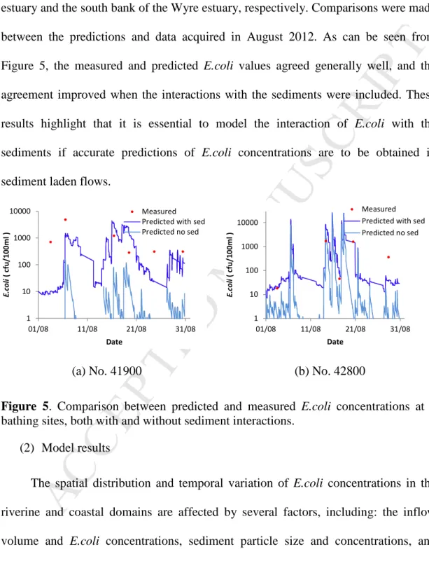
17Figure 5 shows the E.coli predictions using the original model without coupling to 1
the sediments, with the predicted and measured E.coli concentrations being compared 2
at two bathing water sites (No. 41900 and 42800) near the north bank of Ribble 3
estuary and the south bank of the Wyre estuary, respectively. Comparisons were made 4
between the predictions and data acquired in August 2012. As can be seen from 5
Figure 5, the measured and predicted E.coli values agreed generally well, and the 6
agreement improved when the interactions with the sediments were included. These 7
results highlight that it is essential to model the interaction of E.coli with the 8
sediments if accurate predictions of E.coli concentrations are to be obtained in 9
sediment laden flows. 10
(a) No. 41900 (b) No. 42800
Figure 5. Comparison between predicted and measured E.coli concentrations at 2 11
bathing sites, both with and without sediment interactions. 12
(2) Model results
13
The spatial distribution and temporal variation of E.coli concentrations in the 14
riverine and coastal domains are affected by several factors, including: the inflow 15
volume and E.coli concentrations, sediment particle size and concentrations, and 16
environmental conditions, such as light intensity, wind speed etc. The spatial 17
distributions of the modelled E.coli concentrations are shown for low and high tides in 18
Figure 6, both with sediment coupling (Figures 6a, c) and without sediment coupling 19 1 10 100 1000 10000 01/08 11/08 21/08 31/08 E .c o li ( cf u /1 0 0 m l ) Date Measured Predicted with sed Predicted no sed 1 10 100 1000 10000 01/08 11/08 21/08 31/08 E .c o li ( cf u /1 0 0 m l ) Date Measured Predicted with sed Predicted no sed
M
AN
US
CR
IP
T
AC
CE
PT
ED
18(Figures 6b, d). The results show that the relative high E.coli concentration regions, 1
with a concentration in the range exceeding 500 cfu/100 ml, are located mainly in the 2
river deltas, salt marshes and a part of the beach. The high concentration regions may 3
move to and fro along the river corridor and coastline, controlled by the river flow and 4
tidal currents (Figure 6 a, c). The middle concentration region, where the E.coli 5
concentration ranges from 200 to 800 cfu/100 ml, tends to move in a south-westerly 6
direction, along the river corridor, controlled mainly by the river flow. The front of 7
the middle concentration region may reach Southport, to the south of the estuary 8
(Figure 6 c). In addition, under some conditions, e.g. strong southerly winds and 9
currents, the middle concentration region may also occasionally reach the Fylde Coast 10
to the North. The low concentration region appears in the estuary, with these 11
conditions primarily occurring at neap tides and for large river discharges. The local 12
point sources near the bathing water sites may also have some impact on the E.coli 13
concentrations locally. 14
From the model predicted E.coli concentration distributions, both with and 15
without sediment coupling, it can be seen that the sediment transport processes may 16
play an important role in the E.coli surviving rate by changing the sunlight radiation 17
effects and by sediment: advection, deposition and erosion, and adsorption and 18
desorption of the FIOs to/from the sediments. The E.coli bacteria attached to the 19
surface of sediment particles can be transported more readily to the offshore marine 20
waters as an additional net source of E.coli (Zhongfu et al., 2010), while the free 21
swimming E.coli component is much more likely to stay within the coastal zone. This 22
means that E.coli concentrations will generally be underestimated without including 23
the coupling sediment processes of adsorption and desorption, especially in the 24
offshore region. Furthermore, since the E.coli concentration is regularly predicted and 25
M
AN
US
CR
IP
T
AC
CE
PT
ED
19measured to be relatively high in the intertidal region, more E.coli bacteria are likely 1
to be attached to the sediment particles. The resuspension and subsequent movement 2
with tidal currents then delivers the E.coli bacteria to the nearshore region, resulting 3
in a likely further increase in the E.coli concentration levels in this region. 4
M
AN
US
CR
IP
T
AC
CE
PT
ED
20(a) With sediment coupling, at low water neap tide
(b) Without sediment coupling, at low water neap
tide x(m) y (m ) 300000 350000 400000 380000 400000 420000 440000 460000 480000 600 570 540 510 480 450 420 390 360 330 300 270 240 210 180 150 120 90 60 30 0 Tidal level: m Wind Mag: m/s E.coli (cfu/100 ml) Date: 0 5 10 15 20 25 30 Wind Dir: Radiation Watts/m^2 Rainfall: mm/hr Total inflow m^3/s Ribble Inflow: m^3/s Humidity: % Temperature Deg. Cloud: Fractional 6.0 4.0 2.0 0.0 -2.0 -4.0 -6.0 Time(d) T id a l le v e l (m ) 05 0 05 5 06 0 07 0 075 080090 100 120 130 150 180 190 210230 250 260 280 300 310 326355 420 430 440 450459 2012-08-06 07:30:00 2.91 638. 0.8 0.0 91.3 11.4 482.8 38.9 -3.7 x(m) y (m ) 300000 350000 400000 380000 400000 420000 440000 460000 480000 600 570 540 510 480 450 420 390 360 330 300 270 240 210 180 150 120 90 60 30 0 Tidal level: m Wind Mag: m/s E.coli (cfu/100 ml) Date: 0 5 10 15 20 25 30 Wind Dir: Radiation Watts/m^2 Rainfall: mm/hr Total inflow m^3/s Ribble Inflow: m^3/s Humidity: % Temperature Deg. Cloud: Fractional 6.0 4.0 2.0 0.0 -2.0 -4.0 -6.0 Time(d) T id a l le v e l (m ) 05 0 05 5 06 0 07 0 075 080090 100 120 130 150 180 190 210230 250 260 280 300 310 326355 420 430 440 450459 2012-08-06 07:30:00 2.91 638. 0.8 0.0 91.3 11.4 482.8 38.9 -3.7
M
AN
US
CR
IP
T
AC
CE
PT
ED
21(c) With sediment coupling, at high water spring tide
(d) Without sediment coupling, at high water spring tide
Figure 6. Spatial distributions of predicted E.coli: with (a and c), and without (b 1
and d) sediment coupling on 6th August, 2012
2 3 x(m) y (m ) 300000 350000 400000 380000 400000 420000 440000 460000 480000 600 570 540 510 480 450 420 390 360 330 300 270 240 210 180 150 120 90 60 30 0 Tidal level: m Wind Mag: m/s E.coli (cfu/100 ml) Date: 0 5 10 15 20 25 30 Wind Dir: Radiation Watts/m^2 Rainfall: mm/hr Total inflow m^3/s Ribble Inflow: m^3/s Humidity: % Temperature Deg. Cloud: Fractional 6.0 4.0 2.0 0.0 -2.0 -4.0 -6.0 Time(d) T id a l le v e l (m ) 05 0 05 5 06 0 07 0 075 0 80090 1 00 120 130 150 180 190 210230 250 260 280 300 310 326355 420 430 440 450459 2012-08-06 13:30:00 2.65 1474. 0.7 0.0 79.2 13.2 428.2 37.3 3.2 x(m) y (m ) 300000 350000 400000 380000 400000 420000 440000 460000 480000 600 570 540 510 480 450 420 390 360 330 300 270 240 210 180 150 120 90 60 30 0 Tidal level: m Wind Mag: m/s E.coli (cfu/100 ml) Date: 0 5 10 15 20 25 30 Wind Dir: Radiation Watts/m^2 Rainfall: mm/hr Total inflow m^3/s Ribble Inflow: m^3/s Humidity: % Temperature Deg. Cloud: Fractional 6.0 4.0 2.0 0.0 -2.0 -4.0 -6.0 Time(d) T id a l le v e l (m ) 05 0 05 5 06 0 07 0 075 080090 100 120 130 150 180 190 210230 250 260 280 300 310 326355 420 430 440 450459 2012-08-06 13:30:00 2.65 1474. 0.7 0.0 79.2 13.2 428.2 37.3 3.2
M
AN
US
CR
IP
T
AC
CE
PT
ED
222.3 Evaluation of effectiveness of management plans 1
In order to evaluate the effectiveness of the proposed management plans for E.coli 2
concentration reductions in estuarine and coastal regions 6 scenario runs were carried 3
out. The details of the 6 designed scenarios are listed as follows: (i) Scenario A: 4
baseline plus FIO loads to the urban networks since summer 2012; (ii) Scenario B: all 5
major urban areas improved to a level consistent with plans for Preston/Blackburn to 6
2020 (urban flux 50% reduction); (iii) Scenario C: rural improvement (rural flux: 50% 7
reduction); (iv) Scenario D, E, F: up to 1000 m extension of 5 key main outfalls 8
toward the open sea, according to the plans outlined by the local water company and 9
the Environment Agency, while the E.coli inputs from the upstream catchments are 10
kept the same as for Scenarios A, B, C respectively. The E.coli and sediment coupled 11
model was used in the scenario runs based on the data acquired during August, 2012. 12
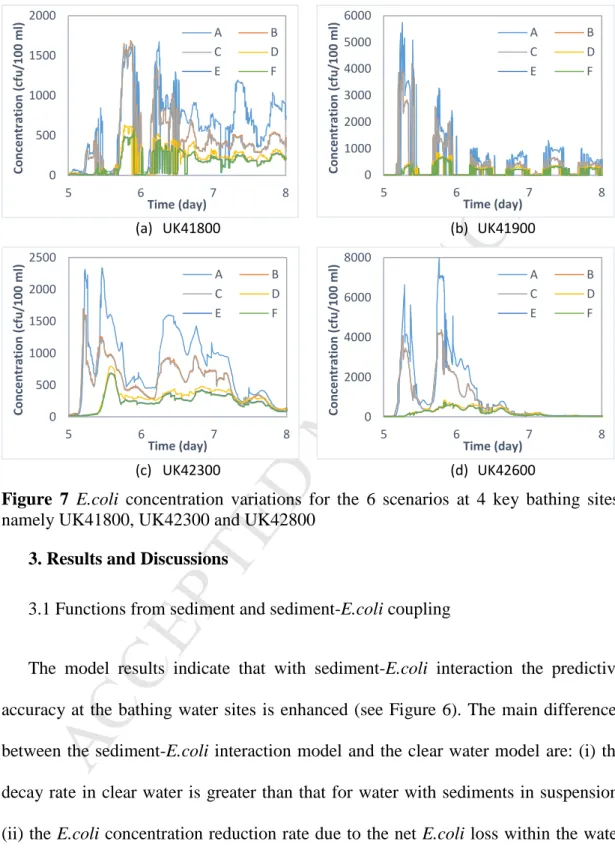
The predicted E.coli concentration values at the key bathing water sites, namely 13
UK41800, UK42300 and UK42800, are presented in Figure 8. The main results can 14
be summarised as follows: (i) the scenarios leading to a 50% cutoff in the urban flux 15
and outfall extension are effective in reducing the E.coli concentrations at the bathing 16
water sites (see Figure 8), with the E.coli concentrations being reduced to about 1/3rd
17
of their original values and with the peak value being reduced to 500~1000 cfu/100ml, 18
which is close to the upper-limit of the new EU bathing water standard (500 19
cfu/100ml); (ii) the extension of the outfalls is more effective than other measures in 20
reducing the peak value of the E.coli concentration; and (iii) the 50% cutoff of the 21
rural sources in the catchments near the Wyre delta to the Ribble delta is not effective 22
at the bathing water sites near Blackpool, since the high urbanized intensity in this 23
region, and the ratio of the rural source input, is an order of magnitude smaller when 24
compared to the urban E.coli sources. Comparisons with the new EU bathing water 25
M
AN
US
CR
IP
T
AC
CE
PT
ED
23quality standards, and the effectiveness of these various schemes, will be further 1
analyzed in the next section using the accumulated probability calculation. 2
(a) UK41800 (b) UK41900
(c) UK42300 (d) UK42600
Figure 7 E.coli concentration variations for the 6 scenarios at 4 key bathing sites, 3
namely UK41800, UK42300 and UK42800 4
3. Results and Discussions 5
3.1 Functions from sediment and sediment-E.coli coupling 6
The model results indicate that with sediment-E.coli interaction the predictive 7
accuracy at the bathing water sites is enhanced (see Figure 6). The main differences 8
between the sediment-E.coli interaction model and the clear water model are: (i) the 9
decay rate in clear water is greater than that for water with sediments in suspension; 10
(ii) the E.coli concentration reduction rate due to the net E.coli loss within the water 11
column is an order of magnitude smaller than the reduction caused by dilution due to 12
advection and diffusion (Pramod et al., 2010); and (iii) the time dependent transport 13 0 500 1000 1500 2000 5 6 7 8 C o n ce n tr a ti o n ( cf u /1 0 0 m l) Time (day) A B C D E F 0 1000 2000 3000 4000 5000 6000 5 6 7 8 C o n ce n tr a ti o n ( cf u /1 0 0 m l) Time (day) A B C D E F 0 500 1000 1500 2000 2500 5 6 7 8 C o n ce n tr a ti o n ( cf u /1 0 0 m l) Time (day) A B C D E F 0 2000 4000 6000 8000 5 6 7 8 C o n ce n tr a ti o n ( cf u /1 0 0 m l) Time (day) A B C D E F
M
AN
US
CR
IP
T
AC
CE
PT
ED
24and resuspension of sediment particles, which are associated with E.coli adsorption 1
and desorption to the sediments, may further change the movement of E.coli. In 2
comparison with the clear water model, the model results with sediment coupling are 3
found to be closer in agreement with the measured E.coli concentrations and a 4
smoother transformation occurs between the maximum and minimum values (see 5
Figure 5). Without sediment coupling, the minor peaks and low values due to the 6
E.coli desorption and adsorption with the sediments may disappear.
7
3.2 Effectiveness of management plans 8
Based on a probability analysis of the results shown in Figure 8, the E.coli 9
reductions for the various management and engineering scenarios maintain the same 10
trends as shown in Figure 7. Furthermore, any extension of the outfall is predicted to 11
be more effective in reducing the peak E.coli value, which is sensitive to the distance 12
between the bathing water beach and the outfall sites. After implementation of the 13
combined sewage extension plan, the E.coli concentration value at the 95% 14
probability level will be less than 500 cfu/100ml, except at the bathing water site 15
named UK42600, which, however, has shows a substantial reduction from 2300 16
cfu/100ml to 550 cfu/100 ml for the worst case scenario. This means that the 17
microbiological compliance with the new EU Bathing Water standard (maximum 500 18
cfu with 95% probability level for E.coli in estuarine bathing waters) can be improved 19
significantly with outfall extensions. According to the model predictions, the outfall 20
extensions taken further offshore are preferable for spring tide conditions in order to 21
satisfy the new EU bathing water standards. Moreover, due to the large proportion of 22
urban FIO sources in the catchments, the urban source cutoff will also play an 23
important role in reducing E.coli inputs. However, a 50% cutoff in the urban source 24
M
AN
US
CR
IP
T
AC
CE
PT
ED
25alone does not seem to be not sufficient to enable the bathing water quality along the 1
Ribble estuary and coast to satisfy the new EU standard. 2
(a) UK41800 (b) UK41900
(c) UK42300 (d) UK42600
Figure 8 Accumulated probability analysis results for the 6 scenarios at 4 key bathing 3
water sites, namely UK41800, UK41900, UK42300 and UK42600. 4
4. Conclusions 5
In natural marine and aquatic waters the fate and transport processes of FIOs are 6
highly dynamic and complex and they can vary significantly from the upstream 7
catchments to the coastal regions. In the current study an integrated numerical 8
modelling system has been refined and applied to predict the spatial and temporal 9
distribution of FIOs in riverine basins and, in particular, coastal bathing waters. The 10
integrated model includes the river network (RNM1D) model and the open source 11
2D/3D EFDC model, in which the upper boundaries are specified from the results for 12 0 500 1000 1500 2000 60 70 80 90 100 C o n ce n tr a ti o n ( cf u /1 0 0 m l) Probability (%) A B C D E F 95 0 1000 2000 3000 4000 5000 6000 60 70 80 90 100 C o n ce n tr a ti o n ( cf u /1 0 0 m l) Probability (%) A B C D E F 95 0 500 1000 1500 2000 2500 60 70 80 90 100 C o n ce n tr a ti o n ( cf u /1 0 0 m l) Probability (%) A B C D E F 95 0 2000 4000 6000 8000 60 70 80 90 100 C o n ce n tr a ti o n ( cf u /1 0 0 m l) Probability (%) A B C D E F 95
M
AN
US
CR
IP
T
AC
CE
PT
ED
26two catchment models for rural regions and the Inforworks model for urban regions. 1
The key refinement to the existing codes is the inclusion of FIO interactions between 2
the water column and suspended sediments. The modelling system was applied to 11 3
catchments of the river Ribble basin and the coastal receiving water of the Liverpool 4
Sea, UK, with model predictions being compared with field measurements taken 5
along the Ribble river and estuary in 1999 and 2012. The level of agreement between 6
the measured and predicted hydrodynamic, sediment transport and E.coli parameters 7
were encouraging at most of the sites. 8
Because the integrated model covers all of the important sub-catchments and 9
better represents the fate and transport processes of FIOs from the source region to the 10
coastal receiving waters, it has the potential to provide more accurate solutions than 11
non-integrated models, particularly for large and complex river basins. Due to the 12
different coding formats and time steps in the sub-systems, a simple linkage approach 13
using input and output data modes was used to link the different sub-systems. Since 14
the 2D model domain was extended to the tidal current limits for the riverine inflows, 15
and due to the relatively large spatial scales used in the current research study, the 16
errors related to this aspect of the study were considered to be small. However, further 17
research needs to be carried out to investigate the impact of stronger dynamic 18
coupling problems. 19
The results confirm that sediment transport is a key process by which FIOs can be 20
transported from river basins to coastal waters. The concentration distribution of FIOs 21
in coastal and estuarine waters, and exclusion of the transport mechanism of FIOs 22
through adsorption and desorption with the sediments, can lead to a marked under-23
prediction of the FIO levels along coastal waters, and particularly at regions near 24
bathing water sites. The higher FIO levels near bathing water sites appears to be 25
M
AN
US
CR
IP
T
AC
CE
PT
ED
27influenced by the resuspension of sediment particles and the subsequent movement 1
with tidal currents in the offshore direction. 2
The analysis of 6 scenarios in the current study indicated that a significant 3
reduction in the E.coli levels can be obtained by extending outfalls and/or 4
significantly reducing the E.coli source inputs from urban regions. The cumulative 5
analysis showed that the level of compliance with the new EU standard can be 6
improved to a large degree by extending outfalls. Although the emphasis of the work 7
reported herein has focused on the river Ribble Basin and Fylde Coast, the modelling 8
developments are generic and can be applied to other river basin to coast studies, both 9
elsewhere in the UK and internationally. 10
Author Contributions 11
Roger Falconer and Binliang Lin developed the original ideas and Guoxian Huang 12
undertook the studies and further developed and improved on the original ideas as 13
reported herein. Guoxian Huang and Roger Falconer drafted the manuscript, which 14
was revised substantially by all authors. 15
Conflicts of Interest 16
The authors declare no conflict of interest. 17
Acknowledgements 18
This work was supported by the Natural Environment Research Council, the 19
Medical Research Council, the Department for Environment, Food and Rural Affairs 20
and the Economic and Social Research Council, GR NE/I008306/1, UK. The authors 21
are also grateful to the Environment Agency North West and Intertek Energy & Water 22
M
AN
US
CR
IP
T
AC
CE
PT
ED
28Consultancy Services for their provision of data and to all colleagues from the 1
universities of Aberystwyth and Sheffield working on the NERC C2C project. 2
References 3
Ackerman, D., Weisberg, S.B., 2003. Relationship between rainfall and beach 4
bacterial concentrations on Santa Monica Bay beaches. Journal of Water and Health 5
1, 85-89 6
Arnold, J., Fohrer, N., 2005. SWAT2000: current capabilities and research 7
opportunities in applied watershed modelling. Hydrol Process 19, 563-572 doi:DOI: 8
10.1002/hyp.5611 9
Bedri, Z., Corkery, A., O'Sullivan, J.J., Alvarez, M.X., Erichsen, A.C., Deering, L.A., 10
Demeter, K., O'Hare, G.M., Meijer, W.G., Masterson, B., 2014. An integrated 11
catchment-coastal modelling system for real-time water quality forecasts. Environ 12
Modell Softw 61, 458-476 doi:http://dx.doi.org/10.1016/j.envsoft.2014.02.006 13
Bedri, Z., Corkery, A., O'Sullivan, J.J., Deering, L.A., Demeter, K., Meijer, W.G., 14
O'Hare, G., Masterson, B., 2016. Evaluating a microbial water quality prediction 15
model for beach management under the revised EU Bathing Water Directive. J 16
Environ Manage 167, 49-58 doi:http://dx.doi.org/10.1016/j.marpolbul.2014.11.008 17
Benham, B., Baffaut, C., Zeckoski, R., Mankin, K., Pachepsky, Y., Sadeghi, A., 18
Brannan, K., Soupir, M., Habersack, M., 2006. Modeling bacteria fate and transport in 19
watersheds to support TMDLs. T Asae 49, 987-1002 20
Bicknell, B., Imhoff, J., Kittle, J., Donigian, A., Johanson, R., 1997. Hydrological 21
Simulation Program — FORTRAN: User's Manual for Version 11. 22
Boehm, A., Grant, S., Kim, J., Mowbray, S., McGee, C., Clark, C., Foley, D., 23
Wellman, D., 2002. Decadal and shorter period variability of surf zone water quality 24
at Huntington Beach, California. Environ Sci Technol 36, 3885-3892 25
doi:http://dx.doi.org/10.1021/es020524u 26
Byappanahalli, M.N., Nevers, M.B., Whitman, R.L., Ge, Z., Shively, D., Spoljaric, 27
A., Przybyla-Kelly, K., 2015. Wildlife, urban inputs, and landscape configuration are 28
responsible for degraded swimming water quality at an embayed beach. J Great Lakes 29
Res 41, 156-163 doi:http://dx.doi.org/10.1016/j.jglr.2014.11.027 30
Chan, S., Thoe, W., Lee, J., 2013. Real-time forecasting of Hong Kong beach water 31
quality by 3D deterministic model. Water Res 47, 1631-1647
32
doi:http://dx.doi.org/10.1016/j.watres.2012.12.026 33
Cho, K.H., Pachepsky, Y.A., Kim, J.H., Kim, J.-W., Park, M.-H., 2012. The modified 34
SWAT model for predicting fecal coliforms in the Wachusett Reservoir Watershed, 35
USA. Water Res 46, 4750-4760 doi:http://dx.doi.org/10.1016/j.watres.2012.05.057 36
Converse, R.R., Kinzelman, J.L., Sams, E.A., Hudgens, E., Dufour, A.P., Ryu, H., 37
Santo-Domingo, J.W., Kelty, C.A., Shanks, O.C., Siefring, S.D., 2012. Dramatic 38
improvements in beach water quality following gull removal. Environ Sci Technol 46, 39
10206-10213 doi:http://dx.doi.org/10.1021/es302306b 40
M
AN
US
CR
IP
T
AC
CE
PT
ED
29Davies, C.M., Long, J., Donald, M., Ashbolt, N.J., 1995. Survival of fecal 1
microorganisms in marine and freshwater sediments. Appl Environ Microb 61, 1888-2
1896 3
de Brauwere, A., de Brye, B., Servais, P., Passerat, J., Deleersnijder, E., 2011. 4
Modelling Escherichia coli concentrations in the tidal Scheldt river and estuary. Water 5
Res 45, 2724-2738 doi:http://dx.doi.org/10.1016/j.watres.2011.02.003 6
de Brauwere, A., Gourgue, O., de Brye, B., Servais, P., Ouattara, N.K., Deleersnijder, 7
E., 2014a. Integrated modelling of faecal contamination in a densely populated river– 8
sea continuum (Scheldt River and Estuary). Sci Total Environ 468–469, 31-45 9
doi:http://dx.doi.org/10.1016/j.scitotenv.2013.08.019 10
de Brauwere, A., Ouattara, N.K., Servais, P., 2014b. Modeling fecal indicator bacteria 11
concentrations in natural surface waters: a review. Crit Rev Env Sci Tec 44, 2380-12
2453 doi:http://dx.doi.org/10.1080/10643389.2013.829978 13
Fan, J., Ming, H., Li, L., Su, J., 2015. Evaluating spatial-temporal variations and 14
correlation between fecal indicator bacteria (FIB) in marine bathing beaches. Journal 15
of water and health 13, 1029-1038 doi:10.2166/wh.2015.031 16
Field, K.G., Samadpour, M., 2007. Fecal source tracking, the indicator paradigm, and 17
managing water quality. Water Res 41, 3517-3538
18
doi:http://dx.doi.org/10.1016/j.watres.2007.06.056 19
Galperin, B., Kantha, L., Hassid, S., Rosati, A., 1988. A quasi-equilibrium turbulent 20
energy model for geophysical flows. J Atmos Sci 45, 55-62 21
Gao, G., Falconer, R.A., Lin, B., 2013. Modelling importance of sediment effects on 22
fate and transport of enterococci in the Severn Estuary, UK. Mar Pollut Bull 67, 45-54 23
doi:http://dx.doi.org/10.1016/j.marpolbul.2012.12.002 24
Garzio-Hadzick, A., Shelton, D.R., Hill, R.L., Pachepsky, Y.A., Guber, A.K., 25
Rowland, R., 2010. Survival of manure-borne E. coli in streambed sediment: Effects 26
of temperature and sediment properties. Water Res 44, 2753-2762
27
doi:http://dx.doi.org/10.1016/j.watres.2010.02.011 28
Griffith, J.F., Cao, Y., McGee, C.D., Weisberg, S.B., 2009. Evaluation of rapid 29
methods and novel indicators for assessing microbiological beach water quality. 30
Water Res 43, 4900-4907 doi:http://dx.doi.org/10.1016/j.watres.2009.09.017 31
Hamrick, J.M., 1992. A three-dimensional environmental fluid dynamics computer 32
code: Theoretical and computational aspects. Virginia Institute of Marine Science, 33
College of William and Mary. 34
Huang, G., Falconer, R.A., Boye, B.A., Lin, B., 2015a. Cloud to coast: integrated 35
assessment of environmental exposure, health impacts and risk perceptions of faecal 36
organisms in coastal waters. International Journal of River Basin Management, 1-14 37
doi:http://dx.doi.org/10.1080/15715124.2014.963863 38
Huang, G., Falconer, R.A., Lin, B., 2015b. Integrated River and Coastal Flow, 39
Sediment and Escherichia coli Modelling for Bathing Water Quality. Water 7, 4752-40
4777 doi:10.3390/w7094752 41
Huang, G., Zhou, J., Lin, B., Xu, X., Zhang, S., 2016. Modelling flow in the middle 42
and lower Yangtze River, China. Water Management, 1-12
43
doi:http://dx.doi.org/10.1680/jwama.15.00123 44
M
AN
US
CR
IP
T
AC
CE
PT
ED
30Kashefipour, S.M., Lin, B., Harris, E., Falconer, R.A., 2002. Hydro-environmental 1
modelling for bathing water compliance of an estuarine basin. Water Res 36, 1854-2
1868 doi:http://dx.doi.org/10.1016/S0043-1354(01)00396-7 3
Liao, H., Krometis, L.-A.H., Kline, K., Hession, W., 2015. Long-term impacts of 4
bacteria–sediment interactions in watershed-scale microbial fate and transport 5
modeling. J Environ Qual 44, 1483-1490 doi:10.2134/jeq2015.03.0169 6
Liu, L., Fu, X., Wang, G., 2013. Parametric study of fate and transport model of E. 7
coli in the nearshore region of southern Lake Michigan. J Environ Eng 140, 8
A5013001 9
Mellor, G.L., Yamada, T., 1982. Development of a turbulence closure model for 10
geophysical fluid problems. Rev Geophys 20, 851-875 doi:DOI:
11
10.1029/RG020i004p00851 12
Niu, J., Phanikumar, M.S., 2015. Modeling watershed-scale solute transport using an 13
integrated, process-based hydrologic model with applications to bacterial fate and 14
transport. J Hydrol 529, 35-48 doi:http://dx.doi.org/10.1016/j.jhydrol.2015.07.013 15
Obiri‐Danso, K., Jones, K., 1999. The effect of a new sewage treatment plant on
16
faecal indicator numbers, campylobacters and bathing water compliance in 17
Morecambe Bay. J Appl Microbiol 86, 603-614
doi:10.1046/j.1365-18
2672.1999.00703.x 19
Ouattara, N.K., de Brauwere, A., Billen, G., Servais, P., 2013. Modelling faecal 20
contamination in the Scheldt drainage network. J Marine Syst 128, 77-88 21
doi:http://dx.doi.org/10.1016/j.jmarsys.2012.05.004 22
Phillips, A., 2014. Rural HSPF modelling Technical Guide, p. 105. 23
Pramod, T., Phanikumar, M.S., Dmitry, B., Schwab, D.J., Nevers, M.B., Whitman, 24
R.L., 2010. Budget analysis of Escherichia coli at a Southern Lake Michigan Beach. 25
Environ Sci Technol 44, 1010-1016 doi:10.1021/es902232a 26
Rico-Ramirez, M.A., Liguori, S., Schellart, A.N.A., 2015. Quantifying radar-rainfall 27
uncertainties in urban drainage flow modelling. J Hydrol 528, 17-28 28
doi:http://dx.doi.org/10.1016/j.jhydrol.2015.05.057 29
Safaie, A., Wendzel, A., Ge, Z., Nevers, M.B., Whitman, R.L., Corsi, S.R., 30
Phanikumar, M.S., 2016. Comparative Evaluation of Statistical and Mechanistic 31
Models of Escherichia coli at Beaches in Southern Lake Michigan. Environ Sci 32
Technol 50, 2442-2449 doi:10.1021/acs.est.5b05378 33
Shepherd, W., Phillips, A., Stapleton, C., Kay, D., Saul, A., Lerner, D, 2015. 34
Integrated Modelling of Faecal Indicator Organisms (FIOs) for Prediction of Bathing 35
Water Quality, Proceedings of 10th International Urban Drainage Modelling (UDM) 36
conference, Quebec, Canada, 20th-23rd September, Quebec, Canada, pp. 1-10.
37
Thoe, W., Wong, S.H., Choi, K., Lee, J.H.W., 2012. Daily prediction of marine beach 38
water quality in Hong Kong. Journal of hydro-environment research 6, 164-180 39
doi:10.1016/j.jher.2012.05.003 40
Thupaki, P., Phanikumar, M.S., Schwab, D.J., Nevers, M.B., Whitman, R.L., 2013. 41
Evaluating the role of sediment ‐ bacteria interactions on Escherichia coli
42
concentrations at beaches in southern Lake Michigan. Journal of Geophysical 43
Research: Oceans 118, 7049-7065 doi:10.1002/2013JC008919 44
M
AN
US
CR
IP
T
AC
CE
PT
ED
31Wallingford Software Ltd, 1995. HydroWorks on-line documentation
1
Wallingford,HR, UK, in: Ltd, W.S. (Ed.). 2
Wither, A., Rehfisch, M., Austin, G., 2005. The impact of bird populations on the 3
microbiological quality of bathing waters. Water Science & Technology 51, 199-207 4
Wright, M.E., Solo-Gabriele, H.M., Elmir, S., Fleming, L.E., 2009. Microbial load 5
from animal feces at a recreational beach. Mar Pollut Bull 58, 1649-1656 6
doi:10.1016/j.marpolbul.2009.07.003 7
Yakirevich, A., Pachepsky, Y.A., Guber, A.K., Gish, T.J., Shelton, D.R., Cho, K.H., 8
2013. Modeling transport of Escherichia coli in a creek during and after artificial 9
high-flow events: Three-year study and analysis. Water Res 47, 2676-2688 10
doi:http://dx.doi.org/10.1016/j.watres.2013.02.011 11
Yang, L., Lin, B., Kashefipour, S., Falconer, R., 2002. Integration of a 1-D river 12
model with object-oriented methodology. Environ Modell Softw 17, 693-701 13
doi:S1364-8152(02)00029-4 14
Zhongfu, G., Nevers, M.B., Schwab, D.J., Whitman, R.L., 2010. Coastal loading and 15
transport of Escherichia coli at an embayed beach in Lake Michigan. Environ Sci 16
Technol 44, 6731-6737 doi:10.1021/es100797r 17
Zhou, J., Falconer, R.A., Lin, B., 2014. Refinements to the EFDC model for 18
predicting the hydro-environmental impacts of a barrage across the Severn Estuary. 19
Renew Energ 62, 490-505 doi:http://dx.doi.org/10.1016/j.renene.2013.08.012 20
21 22