Estimation of an indicator of the representativeness of survey response

(1)

Natalie Shlomo, Chris J. Skinner and Barry Schouten

Estimation of an indicator of the

representativeness of survey response

Article (Accepted version)

(Refereed)

Original citation:

Shlomo, Natalie and Skinner, Chris J. and Schouten, Barry (2012) Estimation of an indicator of

the representativeness of survey response.Journal of statistical planning and inference, 142 (1).

This version available at: http://eprints.lse.ac.uk/39124/ Available in LSE Research Online: November 2011

LSE has developed LSE Research Online so that users may access research output of the School. Copyright © and Moral Rights for the papers on this site are retained by the individual authors and/or other copyright owners. Users may download and/or print one copy of any article(s) in LSE Research Online to facilitate their private study or for non-commercial research. You may not engage in further distribution of the material or use it for any profit-making activities or any commercial gain. You may freely distribute the URL (http://eprints.lse.ac.uk) of the LSE Research Online website.

This document is the author’s final manuscript accepted version of the journal article, incorporating any revisions agreed during the peer review process. Some differences between this version and the published version may remain. You are advised to consult the publisher’s version if you wish to cite from it.

(2)

Estimation of an Indicator of the Representativeness of Survey

Response

Natalie Shlomo1, Chris Skinner1, Barry Schouten2

1

Southampton Statistical Sciences Research Institute, University of Southampton, Southampton SO17 1BJ, United Kingdom

2

Statistics Netherlands, Henri Faasdreef 312, 2492 JP Den Haag, The Netherlands

Abstract

Nonresponse is a major source of estimation error in sample surveys. The

response rate is widely used to measure survey quality associated with nonresponse,

but is inadequate as an indicator because of its limited relation with nonresponse bias.

Schouten, Cobben and Bethlehem (2009) proposed an alternative indicator, which

they refer to as an indicator of representativeness or R-indicator. This indicator

measures the variability of the probabilities of response for units in the population.

This paper develops methods for the estimation of this R-indicator assuming that

values of a set of auxiliary variables are observed for both respondents and

nonrespondents. We propose bias adjustments to the point estimator proposed by

Schouten et al. (2009) and demonstrate the effectiveness of this adjustment in a

simulation study where it is shown that the method is valid, especially for smaller

sample sizes. We also propose linearization variance estimators which avoid the need

for computer-intensive replication methods and show good coverage in the simulation

study even when models are not fully specified. The use of the proposed procedures is

also illustrated in an application to two business surveys at Statistics Netherlands.

(3)

1. Introduction

One of the most important sources of estimation error in surveys is nonresponse. Survey organisations need indicators of such error for a variety of purposes, for example to compare different surveys, to monitor changes in a repeated survey over time or to monitor changes during the fieldwork of a single survey, perhaps to inform decisions such as when to end fieldwork. An indicator which is widely used for such purposes is the response rate, where a higher response rate is taken to indicate higher quality. However, there has been much recent empirical research (see e.g. Groves (2006), Groves and Peytcheva (2008), Heerwegh, et al. (2007) and references therein) which concludes that the response rate is insufficient as an indicator to measure the potential error arising from nonresponse. Since sample sizes are usually large in surveys, the squared bias component of mean squared error will typically dominate the variance component and hence it is desirable that the indicator reflect nonresponse bias. However, the empirical evidence suggests that the response rate is only a weak predictor of nonresponse bias. There is therefore much interest in survey organisations in the development of alternative indicators (Groves et al., 2008).

In this paper, we consider an indicator proposed by Schouten, Cobben and Bethlemem (2009, referred to hereafter as SCB). The basic idea is that nonresponse bias depends critically on the contrast between the characteristics of respondents and nonrespondents. This contrast can be assessed in terms of the probability of a unit responding to the survey. If all units in the population share the same probability of responding then no nonresponse bias will result and the response mechanism may be viewed as ‘representative’. The indicator proposed by SCB, termed the R-indicator (‘R’ for representativeness), measures the extent to which the response probabilities vary. An advantage of this indicator (shared by the response rate) for various practical applications is that it provides a single measure for the whole survey. It should be recognized that nonresponse bias is defined in relation to a specific population parameter (and hence one or more survey variables). Thus, for any one (multipurpose) survey there may be a very large number of nonresponse biases. It would be

(4)

feasible to construct indicators which are parameter-specific (Groves et al., 2008, Wagner, 2008), but here we suppose the requirement is for a single indicator for the whole survey.

Further discussion of the rationale and applications of the R-indicator is provided by Cobben and Schouten (2007) and Schouten and Cobben (2007) in addition to the paper by SCB. The purpose of this paper is to consider in more detail some of the estimation issues associated with the R-indicator. The R-indicator proposed by SCB is subject to bias arising from the estimation of the response propensities. The bias is particularly problematic for small sample sizes, and a bias adjustment is developed. In addition, we develop linearization variance estimators as an alternative to the method of bootstrapping proposed in SCB. We evaluate these procedures in a simulation study and demonstrate the application of these procedures to a real business survey.

We introduce the theoretical framework and define response propensities in Section 2. The R-indicator is defined at the population level in Section 3. The relation of the R-indicator to non-response bias is discussed in Section 4. Point estimation of the R-indicator using sample data is considered in Section 5. The bias of the point estimator and bias adjustment, variance estimation and confidence intervals are considered in Section 6. A simulation study and results of that study are described in Section 7 and results from a real dataset are demonstrated in Section 8. Finally, we conclude and discuss future work in Section 9.

2. Preliminaries and Response Propensities

We suppose that a sample survey is undertaken, where a sample s is selected

from a finite population U. The units in U are labelled i=1, 2,K,N_{, with the sizes} of s and U denoted n and N , respectively. A probability sampling design is

employed, where s is selected with probability p s . The first order inclusion ( )

probability of unit i is denoted π_i and ₌ −1 i i

(5)

The survey is subject to unit nonresponse, with the set of responding units

denoted r , so r⊂ ⊂s U. We denote summation over the respondents, sample and population by Σ_r , Σ_s and Σ_U , respectively. Let R be the response indicator _i variable so that R_i =1 if unit i responds and R_i =0 , otherwise. Hence,

{ ; _i 1}

r= ∈i s R = . Let X be a vector of auxiliary variables which may influence nonreponse, e.g. a vector consisting of age, gender, degree of urbanization of

residence area and the observed status of the dwelling for a household survey or the

type of business and the number of employees for a business survey.

We define the response propensity

ρ

_i as the conditional expectation (under a model) of R given the values of specified variables, such as the auxiliary variables _i

above, and survey conditions (Little, 1986, 1988). If it is necessary to clarify that the

conditioning is on a vector of variables X , for example, then we write:

( ) ( | ) i i E Rr i i i

ρ ρ

= X x = X =x to denote the conditional expectation of R given that i the vector of variables X for unit i takes the value _i x . Here_i E_r(.) denotes

expectation with respect to the model underlying the response mechanism. We

assume that R is defined for each population unit _i i∈U , so that nonresponse is what Rubin (pp. 30-31, 1987) refers to as ‘stable’, and

ρ

_i is also defined for all i∈U. We also assume that the R_i for different units are independent, conditional on the

specified variables and survey conditions. We shall further assume that the sampling

design and the nonresponse process are ‘unconfounded’ (pp. 35-36, 1987) so that the

probability of selecting s remains ( )p s , whatever the values of the R_i, i∈U. Thus, it is assumed that nonresponse does not depend on the configuration of the sample.

(6)

The variation in the response propensities may be viewed as reflecting the

‘representativeness’ of the nonresponse. In SCB response is defined to be (strongly)

representative if the response propensities are the same for all units in the population, corresponding to the notion of missing completely at random (MCAR) (Little and

Rubin, p. 12, 2002) given the variables which are conditioned upon when defining

ρ

_i. They define a representativeness indicator, termed the R-indicator and denoted R_ρ, in

terms of the population standard deviation of the response propensities:

1 2

( 1) _U( _i _U)

S_ρ = N− −

∑

ρ ρ

− , where ρ_U =

∑

_Uρ_i/N . In order to facilitate the interpretation of the indicator, they define it in terms of S_ρ as follows:

R_ρ = −1 2S_ρ , (3.1)

where this transformation of S_ρ ensures that 0≤R_ρ ≤1 since it may be shown that (1 ) 0.5

U U

S_ρ ≤ ρ −ρ ≤ . The value R_ρ =1 indicates the most representative response, where the

ρ

_i display no variation, and the value 0 indicates the least representative response, where the

ρ

i display maximum variation.

4. Relation of R-Indicator to Non-response Bias

The R-indicator may also be motivated in terms of nonresponse bias. Suppose

that the target of inference is a population mean

θ

=N−1

∑

_U y_i of a survey variable, taking value y_i for unit i and observed only for i∈r. A standard design-weighted estimator of θ is ˆθ =

∑

sd R yi i i/

∑

sd Ri i. The bias of

ˆ

θ

as an estimator of θ may be evaluated by taking expectations with respect to both the random sampling

(7)

We assume, for now, that the specified variables include y so that it may be treated i

as fixed. We then have:

ˆ ( ) / / r s r s i i i i i i i i i s i s i U i U E E θ E E d R y d R ρ y ρ ∈ ∈ ∈ ∈   =  ≈ 

∑



∑

, (4.1) where in this case

ρ

_i =

ρ

_YX(y_i,x_i) is conditional on both Y and X and the

approximation is for large samples so that we take the first term only in the Taylor

expansion. In addition, we have used the assumption that the sampling and response

mechanisms are unconfounded. Hence the bias depends on nonresponse only via

ρ

_i. It follows that ˆ ( ) _i( _i ) / _i i U i U Bias

θ

ρ

y

θ

ρ

∈ ∈ ≈

∑

−

∑

=corr S S_ρ_y _ρ _y/ρ_U, (4.2) where y ( 1) 1 ( i U)( i ) / y i U corr_ρ N −

ρ ρ

y

θ

S S_ρ ∈ = −

∑

− − and y2 ( 1) 1 ( i )2 i U S N − y

θ

∈ = −

∑

− .

Expression (4.2) is also obtained in Bethlehem (1988) and Särndal and

Lundström (p.92, 2005). An upper bound for the absolute bias can thus be expressed

in terms of the R-indicator by

(1 ) ˆ | ( ) | / 2 y y U U R S Bias

θ

S S_ρ

ρ

− ≤ = . (4.3) A standardized measure, which is free of y is given by:

(1 ) 2 _U R B ρ

ρ

− = . (4.4) 5. Estimation of R-indicator

We suppose that the data available for estimation purposes consists first of the

(8)

variables), observed only for respondents. Secondly, we suppose that information is

available on the values ( _1, , _2,, , _, )T i = x i x i xK i

x K _{of a vector}

i

X of auxiliary variables for

all sample units, i.e. for both respondents and non-respondents. We refer to this as

sample-based auxiliary information. This is a key assumption and is natural if, for example, the variables making up x are available on a register. Other possible _i

assumptions about the availability of auxiliary information are discussed in Section 9.

Sincey is only observed for respondents, the response propensity conditional _i

on y is generally inestimable without further assumptions. Instead, we propose to _i

take

ρ

_i in the definition of R_ρ in (3.1) as conditional on x , i.e. to set _i

( ) ( | ) i X i E Rr i i i

ρ ρ

= x = X =x .

Nonresponse is missing at random, denoted MAR (Little and Rubin, p.12,

2002), if R_i is conditionally independent of y_i given x . In this case, we have _i

( | , ) ( | ) r i i i r i i

E R y x =E R x and

ρ ρ

i = X( )xi =

ρ

YX( ,yi xi) and so yi may implicitly be included in the conditioning set. Hence the argument used to obtain the bias bound in

(4.3) still applies if MAR holds. The bias bound and the R-indicator itself may,

however, be too conservative. If MAR holds then

ρ

_Y( )y_i =E_r[

ρ

_X( ) |x_i y_i] and: var(

ρ

_i)=var[

ρ

_X( )]x_i =var{ [E

ρ

_X( ) |x_i y_i]}+E{var[

ρ

_X( ) |x_i y_i]}

=var[

ρ

_Y( )]y_i +E{var[

ρ

_X( ) |x_i y_i]} (5.1) The first term on the right hand side of (5.1) represents the variation of the

conditional probabilities

ρ

Y(yi), which we should ideally like to use in the R-indicator if we are only concerned about nonresponse bias for a target parameter defined in

terms of yi alone. The second term represents additional variation which is unrelated

(9)

variability, i.e. noise, in the

ρ

i for that purpose. Kreuter et al. (2010) present examples of auxiliary variables which are predictive of nonresponse but only weakly

predictive of relevant y variables. In such cases, the second term in (5.1) may be i

relatively large and the R-indicator and its associated bias bound may be viewed as

too conservative. It is therefore desirable to select only those auxiliary variables

which are reasonably predictive of at least one of the y variables of key interest in _i

the survey.

One special case occurs when nonresponse is missing completely at random

(MCAR) so that it is independent of both x andi y . In this case, both i

ρ

X( )x i and

ρ

_Y( )y_i are constant so that both terms on the right hand side of (5.1) are zero. Hence, there is no variability in the

ρ

_i and this does, albeit in a degenerate way, capture the fact that there is nothing in the nonresponse process that will lead to

nonresponse bias for estimation related to y . _i

If nonresponse is not MAR then (5.1) no longer holds. Instead,

ρ ρ

_i = _X( )x will _i

represent a smoothed version of

ρ

YX( ,yi x and it is not necessarily the case that i) var(

ρ

_i) will be at least as large as var[

ρ

_Y( )]y_i . Thus, we may fail to capture relevant features of the nonresponse process in the

ρ

_i. In particular, if R is conditionally _i independent ofx given i y then var[i

ρ

Y( )]yi will necessarily be at least as large as var(

ρ

_i), i.e. var[

ρ

_X( )]x_i (following a parallel argument to the MAR case). It may be argued therefore that it is desirable to select the auxiliary variables constituting x _i

in such a way that the MAR assumption holds as closely as possible. In any case, it

must be emphasized that our definition of

ρ ρ

_i = _X( )x relates to a specific choice of _i

(10)

We noted in Section 2 that we define the response propensity conditional on the

survey conditions that apply when the data are collected. We do not make this

conditioning explicit in our notation, but it is crucial to recognize this conditioning

since, as we noted in Section 1, one of the objectives of constructing R-indicators is to

be able to compare the representativeness of different surveys and such comparisons

becomes challenging when the definition of the response propensity for any one

survey is dependent on the conditions with which that survey has been implemented,

for example upon the modes of data collection, the choice of interviewers, the way

these interviewers were trained and work and the contact strategy. Even for a single

survey repeated at different points in time, such conditions may well not remain

constant.

5.1 Nonresponse models

In order to estimate the R-indicator, we first estimate the response

propensities,

ρ

_i =E R( _i|x_i) . To do this, we assume that

ρ

_i depends on x in a _i

parametric way via:

g(

ρ

_i)=x_i'β, (5.2) where g(.) is a specified link function, β is a vector of unknown parameters and x _i

may involve the transformation of the original auxiliary variables for the purpose of

model specification. In particular, we shall consider the logit link function

( ) log[ /(1 )]

g ρ = ρ −ρ leading to the logistic regression model.

We propose to estimate β by pseudo maximum likelihood (Skinner, pp. 80-83,

(11)

1 [ ( ' )] 0 i i i i sd R g − − =

∑

x β x (5.3)

where g−1(.)is the inverse of the link function. One reason for using the design

weights here is because the objective is to estimate an R-indicator which provides a

descriptive measure for the population.

The response propensity

ρ

_i is then estimated by:

1 _ˆ

ˆ_i g ( _i' )

ρ

₌ − _x _β _. _(5.4)

5.2 Estimation of R-indicator

As in SCB, we propose to estimate R_ρ by:

Rˆ_ρ = −1 2Sˆ_ρ , (5.5) where Sˆ_ρ2 =(N−1)−1

∑

_sd_i(

ρ ρ

ˆ_i− ˆ_U)2 , ρˆ_i is defined in (5.4), ˆ

ρ

_U =(

∑

_sd_i

ρ

ˆ_i) /N and N may be replaced by

∑

_sd_i if it is unknown. We refer to the estimator in (5.5) as the SCB estimator.

6. Bias and Confidence Intervals

6.1 Bias and Bias Adjustment

We now consider the bias properties of the SCB estimator ˆR_ρ defined in (5.5).

We shall assume that the vector of auxiliary variables x is given so that no bias can _i

arise from specifying the ‘wrong’ set of auxiliary variables. We note, nevertheless,

that the choice of auxiliary variables is a critical decision in practice and we shall

illustrate empirically in Section 7 how the R-indicator can depend on this choice.

We first consider defining the bias with respect to the sampling mechanism,

(12)

likelihood estimate ˆβ is approximately unbiased for the ‘census’ parameter βUwhich

solves:

∑

_U[R_i−g−1(x_i' )]β x_i =0 (6.1) (Skinner, p. 82, 2003). The approximation here is with respect to an asymptotic

framework, with a sequence of samples and populations with n and N increasing.

This census parameter implies a corresponding response propensity

ρ

_iU =g−1(x_i'β_U)

and R-indicator R_ρ_U , defined in terms of these propensities. We then have

ˆ ( )

s U

E R_ρ ≈R_ρ . The difference R_ρ_U −R_ρ may be viewed as the bias arising from model misspecification.

Instead of defining the bias with respect to just sampling variation we could also

consider the response mechanism. In a parallel way, we may write E E R_r _s(ˆ_ρ)≈R_ρ_U₀, where R_ρ_U₀ is the R-indicator defined in terms of the response propensities

1 0 ( ' 0) iU g i U

ρ

₌ − _x _β _and 0 U

β is the solution of:

1 0 [ _i ( _i' )] _i 0 U

ρ

g − − =

∑

x β x . (6.2)

where

ρ

_i₀ =E R_r( _i|x is the true response propensity given _i) x and we suppose that _i

0 ( _i )

g

ρ

is not necessarily linear in x , as in (5.2), i.e. the latter model may be _i

misspecified. Thus, RρU0−Rρ may be viewed as the bias (with respect to both sampling variation and the response mechanism) arising from model misspecification.

We may expect that RρU RρU0 O Np( 0.5) −

− = so that there will usually be negligible difference in practice between the two measures R_ρ_U −R_ρ or R_ρ_U₀−R_ρ of bias.

In principle, one might consider ways of assessing either of these measures of

(13)

those for some kind of non-parametric regression. We do not pursue this approach

further here, however. Instead we consider the finite sample biasE R(ˆ_ρ)−R_ρ_U, treating U

R_ρ as the parameter of interest, which is equivalent to assuming that the

nonresponse model in (5.2) is correctly specified. We might anticipate that the finite

sample bias of ˆR_ρ will be non-negligible, since ˆR_ρ is defined via the variance of

the ρˆi and we might expect sampling variation in these quantities to inflate this variance. We approximate this finite sample bias of ˆR_ρ by first considering the bias

of Sˆ_ρ2 defined below (5.5).

We use the decomposition:

ˆ ˆ

ˆ_i _U (ˆ_i _i) ( _i _U) ( _U _s) ( _s _U)

ρ ρ

− =

ρ ρ

− +

ρ ρ

− +

ρ

−

ρ

+

ρ ρ

− ,

where

ρ

_s =N−1

∑

_sd_i

ρ

_i and use the approximation E_r(

ρ

ˆ_i)≈

ρ

_i to obtain E_r(

ρ

ˆ_U)≈

ρ

_s

and: 2 2 2 2 2 ˆ ˆ ˆ ˆ [( ) ] ( ) ( ) ( ) ( ) ˆ ˆ 2 ( , ) 2( )( ) ˆ ˆ ( ) ( ) ( ) 2( )( ) r i U r i i U s U r U i U i U s U r i U r i U s U i U s U E V V Cov V ρ ρ ρ ρ ρ ρ ρ ρ ρ ρ ρ ρ ρ ρ ρ ρ ρ ρ ρ ρ ρ ρ ρ ρ − ≈ + − + − + − − − − = − + − + − − − − It follows that 2 1 2 2 ˆ _ˆ ˆ ( ) ( 1) { ( ) ( ) ˆ ₍ ₎ ₂₍ ₎₍ ˆ _)} r s i i U s i r i U s s U s U s s U E S N d d V N N N ρ ρ ρ ρ ρ ρ ρ ρ ρ ρ ρ − ≈ − − + − + − − − −

∑

where ˆN_s =

∑

_sd_i.

Taking expectation also with respect to the sampling design, we obtain:

2 2 1 2 ˆ ( ) s r E E S_ρ ≈S_ρ+ +A A (6.3) where 1 1 s{( 1) s i r(ˆi ˆU)} A =E N− −

∑

d V ρ ρ− 1 2 2 {( 1) [ ˆs( s U) 2( s U)( s ˆs U)]} A =E N− − N ρ ρ− − ρ ρ− Nρ −N ρ

(14)

Both A and 1 A are terms of 2 O(1/ )n and, following standard linearization arguments,

we simplify these expressions by removing terms of lower order. First, A is ₁

asymptotically equivalent to:

1

1 E Ns{ sd Vi r(ˆi)}

λ ₌ −

_∑

ρ _.

Turning to the termA , we may write ₂

2 2

ˆ ₍ ₎ ₂₍ ₎₍ ˆ _{) {}ˆ _{2 }(} ₎ ₂₍ ˆ ₎₍ ₎

s s U s U s s U s s U s s U U

N

ρ ρ

− −

ρ ρ

− N

ρ

−N

ρ

= N − N

ρ ρ

− + N −N

ρ ρ ρ

− and, ignoring terms of lower order, A is asymptotically equivalent to ₂

2 1 2 Es{( s U) } 2 UEs{(N Nˆs 1)( s U)} λ _{≈ −} ρ ρ₋ ₊ ρ − ₋ ρ ρ₋ _{var (} ₎ ₂ 1_{cov (}_ˆ _, ₎ s ρs ρUN s Ns ρs − = − + .

Replacing A and ₁ A in (6.3) by ₂

λ

₁ and

λ

₂ respectively, we obtain

λ λ

₁+ ₂ as the approximate bias of Sˆ_ρ2. We thus propose as a bias-corrected SCB estimator of R_ρ:

1 2

R%_ρ = − S%_ρ. (6.4)

where S%_ρ2 =Sˆ_ρ2− −

λ λ

ˆ₁ ˆ₂ and

λ

ˆ₁ and

λ

ˆ₂ are estimators of

λ

₁ and

λ

₂ respectively. An estimator of

λ

₁ is 1 1 ˆ _{ˆ ˆ}₍ ₎ i r i s N d V λ ₌ −

_∑

ρ _{, where} _{ˆ ˆ}_{( )} r i V

ρ

is an estimator of ˆ ( ) r i

V

ρ

and N may be replaced by Nˆ_s if it is unknown. We propose to use the estimator Vˆ ˆ_r( )

ρ

_i given in the Annex. In the case of constant weights d_i =N n/ this gives: 1 2 1 1 ˆ ₍ _{' )}ˆ _'[ ₍ _{' )}ˆ _'] i i j j j i i s j s n h h λ − − ∈ ∈ =

∑

∇ x β x

∑

∇ x β x x x ,

where ∇h(x_i' )βˆ =exp(x_i' ) /[1 exp(βˆ + x_i' )]βˆ 2.

The second term

λ

₂ may, in general, be estimated using design-based variance estimation methods. In the case of constant weights the term Nˆ_s is constant so

λ

₂

(15)

reduces to λ₂ = −V_s(ρ_s) . Under simple random sampling, we may write

1 1 2

2 (n N )Sρ

λ _{= −} − ₋ − _{. It follows that a bias corrected estimator of} 2

S_ρ in the case of

simple random sampling is:

2 2 1 1 2 1 2 1 1 2 ˆ ˆ ˆ ₍₁ ₎ˆ ₍ _{' )}ˆ _'[ ₍ _{' )}ˆ _'] i i j j j i i s j s S_ρ S_ρ λ λ n− N− S_ρ n− h h − ∈ ∈ = − − = + − −

∑

∇ x β x

∑

∇ x β x x x % _{. (6.5)}

6.2 Standard Errors and Confidence Intervals

A linearization variance estimator for the SCB estimator ˆR_ρ is now derived in

terms of a variance estimator v S(ˆ_ρ2) of Sˆ_ρ2, assuming that a logistic regression model

is fitted and holds. From (5.5) and using linearization we have

2 _ˆ2 ˆ

var[R_ρ]≈S_ρ− var(S_ρ) . (6.6) To approximate var(Sˆ_ρ2) we shall decompose the distribution of Sˆ_ρ2 into the part

induced by the sampling design for a fixed value of ˆβ and the part induced by the

distribution of ˆβ. We take the latter to be ˆβ N( , )β Σ , where:

1 1

( ) var{ sd Ri[ i h( i' )] } ( )i

− −

=

∑

−

Σ J β x β x J β (6.7)

and ( )J β =E{ ( )}I β is the expected information rather than the observed information in (6.7). These two choices of information are asymptotically equivalent (to first order)

but the expected information has the advantage that Σ does not depend on s.

We write

2 2 2

ˆ ˆ

ˆ ˆ ˆ

var(S_ρ)=E_β[var (_s S_ρ)] var [+ _β E S_s( _ρ)], (6.8)

where the subscript ˆβ denotes the distribution induced by ˆβ N( , )β Σ , which may be

interpreted as arising from the response process. Following usual linearization

(16)

2 1 2 ˆ ˆ var (s ) var [s i( i U) ] i s S_ρ N− d

ρ ρ

∈ ≈

∑

− β=β

and, given the consistency of ˆβ for β (and for standard kinds of sampling designs),

we have approximately: 2 1 2 ˆ[var (s ˆ )] var [s i( i U) ] i s E S_ρ N− d

ρ ρ

∈ ≈

∑

− β . (6.9)

Turning to the second component in (6.8), we may write:

2 1 2 ˆ ˆ ( ) ( ) s i U i U E S_ρ N−

ρ ρ

∈ ≈

∑

− β=β .

As a linear approximation we have

ρ ρ

ˆ_i ≈ +_i z_i′(βˆ-β) where z_i = ∇h(x_i' )β x_i. Hence

2 2 ˆ ˆ ( ) ( ) 2 ( )( ) ( ) ˆ ˆ ( ) ( )( ) ( ) i U i U i U i U i U i U i U i U i U i U

ρ ρ

∈ ∈ ∈ ∈ ′ − ≈ − + − − ∑ ∑ ∑ ′ ′ +∑ − − − − β=β z z β-β z z β β β β z z where U N 1 U i − =

∑

z z .

In large samples, we assume that ˆβ is normally distributed so that ˆ(β−β) is uncorrelated with ˆ(β−β β)(ˆ−β) '. Hence, we have

2 ˆ ˆ ˆ ˆ ˆ var [E S_s( _ρ)]≈4 ′ +var { [ (tr )( ) ]}′ β AΣA β B β-β β-β , (6.10) where 1 ( _i _U)( _i _U) i U N− ρ ρ ∈ =

∑

− − A z z , 1 ( _i _U)( _i _U) ' i U N− ∈ =

∑

− B z - z z z and Σ is defined

in (6.7). The second term involves the fourth moments of ˆβ which may also be

expressed in terms of Σ since ˆβ is assumed normally distributed.

The variance of Sˆ_ρ2 may be estimated by the sum of the estimated components of

(6.8). The first of these appears in (6.9) and may be estimated by a standard

design-based estimator of var [_s _i( _i _U) ]2

i s

d

ρ ρ

∈ −

(17)

linear statistic var [_s _i] i s

u ∈

∑

and u is replaced by _i d_i(

ρ ρ

ˆ_i− ˆ_U)2 in the expression for the variance estimator. The second component of the variance appears in (6.10). To

estimate this term requires estimating A , B and Σ. First, z may be estimated by _i

ˆ ˆ_i = ∇h( _i' ) _i

z x β x . Then A may be estimated by ˆ 1 i(î Û)(î Û) i s N− d

ρ ρ

∈ =

∑

− − A z z , B may be estimated by ˆ 1 i(î Û)(î Û) ' i s N− d ∈ =

∑

− − B z z z z , where zˆ_U =N−1

∑

_sd_iz , and ˆ_i Σ may be estimated by a standard estimator of the covariance matrix of ˆβ.

Finally, the variance of the SCB estimator ˆR_ρ may be estimated by plugging the

estimated variance of Sˆ_ρ2 into (6.6) and replacing S_ρ2 by Sˆ_ρ2.

A confidence interval for R_ρ with level 1−α is given by

2 2 0.5

/ 2 ˆ 1 2− S%_ρ ±z_α v S( _ρ) .

7. Simulation Study of the Properties of the estimated R-indicators

7.1 Design of Simulation Study

In this Section, we carry out a simulation study to assess the sampling properties

of the estimation procedures described in Section 6. The study is based on repeated

samples drawn from a file (representing itself a 20% sample) from the 1995 Israel

Census. The file contains 753,711 individuals aged 15 and over in 322,411

households. The samples are drawn using designs intended to be similar to some

standard household and individual surveys carried out at national statistics institutes.

We use the following sample designs in the simulations:

• Household Survey – the sample units are households and all persons over the age of 15 in the sampled households are interviewed. Typically a proxy questionnaire

(18)

is used and therefore there is no individual non-response within the household. In

addition, we assume that every household has an equal probability to be included

in the sample.

• Individual Survey - the sample units are individuals over the age of 15. We assume equal inclusion probabilities.

For each type of survey, we carried out a two-step design to define response

probabilities in the population (census) file. In the first step, we determined

probabilities of response based on explanatory variables that typically lead to

differential nonresponse based on our experiences of working with survey data

collection. A response indicator was then generated for each unit in the population file.

In the second step, we fit a logistic regression model and generate a ‘true’ response

propensity for each unit in the population as predicted by the model. The dependent

variable for the logistic model is the response indicator and the independent variables

of the model the explanatory variables used in the first step (described below). This

two-step design ensures that we have a known model generating the response

propensities in the population and therefore can assess model misspecification besides

the sampling properties of the indicators.

The explanatory variables used to generate the response probabilities are the

following:

• Household Survey – Type of locality (3 categories), number of persons in household (1,2,3,4,5,6+), children in the household indicator (yes, no).

• Individual Survey – Type of locality (3 categories), number of persons in household (1,2,3,4,5,6+), children in the household indicator (yes, no), income

(19)

500 samples of size n were drawn from the Census population of size N at

different sampling fractions 1:50, 1:100, and 1:200. For each sample drawn, a sample

response indicator was generated from the ‘true’ population response probability. The

overall response rate was 82% for the household survey and 78% for the individual

survey. Response propensities and the R-indicator were then estimated from the

sample. Two choices of auxiliary variables were considered, first the ‘true’ variables

employed to generate the response propensities and, second, a simpler set of variables,

intended to represent a possible misspecified model.

7.2 Results

Simulation means of the SCB estimator ˆR_ρ, defined in (5.5), and its proposed

bias corrected version R%_ρ, defined in (6.4), obtained from the 500 repeated samples

drawn for the Household Survey at different sampling rates and for two different

models are reported in Table 1. Corresponding results for the Individual Survey are

presented in Table 2. Also included in the tables is the percentage of Relative Bias

calculated from the simulation study as: 100{[

∑

500_B₌₁(Rˆ_ρB −R_ρ)/R_ρ]/500} where RˆρB is the value ofRˆ computed for the Bth simulation sample and similarly for _ρ R%_ρ.

[PLACE TABLE 1 HERE]

The results for the ‘true’ model provide evidence of downward bias in the SCB

estimator, with the (absolute) size of the bias increasing as the sample size decreases.

This is as expected. Sampling error tends to lead to overestimation of the variability

(20)

R-indicator. We observe that the bias correction reduces the (absolute) bias of the SCB

estimator when the true model holds (although there is some evidence of

over-correction in Table 2 which does not disappear as the sample size increases). The bias

correction decreases (in absolute value) with the increase in sample sizes and tends to

stabilize the SCB estimator.

Using a less complex logistic model to estimate response probabilities results

in a ‘smoothing’ of the probabilities and hence an increase in the value of the

R-indicator. We include in Tables 1 and 2 values ofRρU0, which is the R-indicator for

the logistic model for the reduced set of auxiliary variables which best fits the

response propensities generated by the ‘true’ model (for the complete set of auxiliary

variables) in the population. Treating R_ρ_U₀ as the parameter of interest, we observe

that the bias adjustment does reduce the (absolute) bias for the household survey but

not necessarily for the individual survey, where the bias correction can lead to

overestimation. The instability of the bias correction for the less complex set of

auxiliary variables is likely caused by the misspecification of the model. Since the

bias correction depends on the correct specification of the logistic model, it may not

perform quite so well in these cases.

The Relative Root Mean Square Errors (RRMSE) were also calculated from

the simulation study as: 100{ [ 500(ˆ ) /500]} 1 2 1

∑

= − ₋ B R B R

R_ρ _ρ _ρ but not presented in the

tables. There was no systematic evidence of the bias adjustment leading to larger

RRMSEs. For the Household Survey, the RRMSE was stable across the SCB and

proposed estimators for both types of models. For the Individual Survey, there was

(21)

types of models. This result is reflected by the Relative Bias that is presented in the

tables.

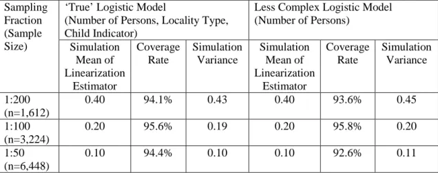
Simulation means of the linearization variance estimator (see Section 6.2) are

compared in Tables 3 and 4 with the simulation variances (calculated across the

replicated samples) of the SCB estimator for the household and individual surveys,

respectively. The tables also include the Coverage Rate defined as the percentage of

times that the trueR_ρ is included in the confidence interval calculated by the

linearization variance estimator: 100{[ 500 ( ˆ 2 var (ˆ ))]/500} 1

∑

_B₌ I Rρ∈RρB ± B RρB where )

ˆ (

var_B R_ρ_B is the estimated linearization variance for the Bth simulation sample and I

is the indicator function.

The linearization variance estimator is seen to be approximately unbiased across the

range of conditions represented in these tables under the different sample sizes with

good coverage as seen by the coverage rate in the tables.

Figures 1 and 2 present box plots comparing the SCB estimator and its proposed

bias adjusted version for the Household and Individual Survey simulation respectively

when fitting the ‘true’ logistic regression model. The gains from the bias adjustment

are evident.

[PLACE FIGURE 1 HERE]

(22)

8. Application to Real Surveys

We demonstrate the use of R-indicators on business surveys undertaken for the

2007 Dutch Short Term Statistics (STS) for retail and industry. Table 5 provides a

brief description of the two surveys.

In the table, the survey response rates are given for 15, 30, 45 and 60 days of

fieldwork. After 30 days STS needs to provide data for monthly statistics. We

examine both a complete set of auxiliary variables consisting of (i) business size class

(based on number of employees), (ii) business sub-type and (iii) VAT 2006 as

collected by the Tax Board and a reduced set consisting of just (i) and (ii). Table 6

provides the results of the unadjusted and bias adjusted R-indicators, 95% confidence

intervals and the standardized maximal bias (obtained by plugging estimated response

propensities into (4.4)) after 15, 30, 45 and 60 days of fieldwork for each of the

business surveys. Because of the large sample size, the bias adjustment had a small

impact.

The samples for the business surveys are large and hence the confidence

intervals are reduced with widths between 1% and 1.5%. The R-indicator for STS

retail after 30 days fieldwork drops almost 7% when VAT is added to the auxiliary

information. For STS industry the decrease is much reduced. Apparently, the size of

VAT in the previous year does not relate to response very strongly. Without the VAT

information the retail respondents have a higher R-indicator than the industry

(23)

worse. STS retail shows a reduction in the R-indicator as the response rates increase

for the reduced set of auxiliary variables. The main survey item of the STS surveys is

monthly turnover (subdivided over different activities). As VAT in a previous year

can be expected to correlate strongly to turnover in the running year, it is important

that representativeness is good with respect to VAT. The main conclusion is that for

Industry, the R-indicator goes up after 30 days, suggesting response

representativeness is still improving and one would ideally wait longer than 30 days

before producing statistics. For Retail, the R-indicator is lower, suggesting that

response is less representative than for Industry, but there is very little change when

data collection is prolonged. Hence, it does not pay off to wait longer

than 30 days considering the composition of the response. The only reason to do so

would be that the risk of nonresponse bias as reflected by the maximal bias is still

decreasing as responses are coming in.

9. Discussion

In this paper we have considered a new indicator, called the R-indicator,

designed to reflect the potential estimation error arising from nonresponse. The

indicator is defined at the population level and we have developed methods for its

estimation using sample data, including methods of bias adjustment and variance

estimation. The approximate validity of these methods has been demonstrated via

simulation. We have also demonstrated how the indicator may be used in real

business surveys as well as social surveys. The bias adjustment is particularly

effective for small sample sizes. In addition, the variance estimation provides good

(24)

The indicator is defined with respect to a set of auxiliary variables. An

R-indicator cannot be viewed separately from the auxiliary vector X that was used to

define it. As such, indicator values should always be reported with reference to the

auxiliary variables. Consequently, when comparing multiple surveys within one

survey institute, over survey institutes or even over countries, one needs to fix the set

of auxiliary variables used for each of the surveys. There are two conflicting aims that

need to be balanced when selecting auxiliary variables in the comparison of different

surveys. On the one hand, it is desirable to choose auxiliary variables that are

maximally correlated with the variables of analytic interest in each survey. On the

other hand, the choice is constrained to the set of auxiliary variables that is available

for each of the surveys. The wider the scope of the comparison, the more restrictive

the availability of variables will be. Within one survey institute one is likely to use

one sampling frame, have access to the same register data and collect similar paradata

for surveys. Multiple countries, however, may have completely different traditions

and legislation, which will limit the set of auxiliary variables that is shared. More

discussion on the selection of auxiliary variables is in Schouten, Shlomo and Skinner

(2011).

A key assumption has been that these variables are measured on both

respondents and nonrespondents. This assumption may be reasonable in some survey

settings. For example, rich auxiliary information is available at Statistics Netherlands

from a population register. However, in other survey settings, the availability of

unit-level auxiliary information on nonrespondents may be very limited. Instead, aggregate

information on the population totals of auxiliary variables may be available. We are

(25)

Acknowledgements

This research was undertaken as part of the RISQ (Representativity Indicators for

Survey Quality) project, funded by the European 7th Framework Programme (FP7),

as a joint effort of the national statistical institutes of Norway, the Netherlands and

Slovenia and the Universities of Leuven and Southampton. We should like to thank

Li-Chun Zhang, Jelke Bethlehem, Mattijn Morren and Ana Marujo for their

(26)

Annex. Variance of ˆ

ρ

_i for logistic regression model

For the logistic regression model, write 1

( ) ( ) exp( ) /[1 exp( )]

hη =g− η = η + η . The estimating equations in (5.3) may then be expressed as:

[ ( ' )] 0

i i i i

sd R −h =

∑

x β x . (A1)

Let ˆβ solve (A1). Then in large samples we may approximate the distribution of ˆβ

with respect to the sampling design (c.f. Skinner, pp. 80-83, 1989) by the distribution

of : 1 ˆ ₍ ₎ _[ ₍ _{) ]} U U sd Ri i h i U i − _′ ≈ +

∑

− β β I β xβ x , (A2)

where β_U is defined in (6.1), ( )I β =

∑

_sd_i∇h(x_i' )β x x is the information matrix and _i _i' ( ) ( ) / ( )[1 ( )]

hη hη η hη hη

∇ = ∂ ∂ = − . In particular, the variance of ˆβ with respect to the sampling design is in large samples

1 1

ˆ

( ) ( ) { [ ( )] } ( )

s U s s i i i U i U

V β ≈I β −V

∑

d R −h x′β x I β − (A3) and, since

ρ

ˆ_i =h(x_i' )βˆ from (5.4), we have

2 _ˆ 2 1 1 ˆ ( ) ( ) ( ) ( ) ( ) { [ ( )] } ( ) s i i U i s i i U i U s j j j U j U i j s V ρ h V h −V d R h − ∈ ′ ′ ′ ′ ′ ≈ ∇ xβ x β x = ∇ xβ x I β

∑

− x β x I β x (A4)

This expression treats the response indicators R_j as fixed. To account for the

response mechanism also, we may write ρ_i₀ =E R_r( _i|x and _i)

ˆ ˆ ˆ

var(ρ_i)=E V_r[ (_s ρ_i)]+V E_r[ _s(ρ_i)] (A5) In large samples, we may write Es(ρˆi)≈h(xi'βU). Assuming ρi0 =E Rr( i|x , we i) may write β_U =β_U₀ +O N_p( −0.5) and V E_r[ _s(ρˆ_i)]=O N( −1). The first term in (A5) is generally of 1

( )

(27)

sampling fraction /n N may be treated as negligible. In this case an expression for

ˆ

var(

ρ

_i) may be obtained by replacing β_U in (A4) by β_U₀.

References

Bethlehem, J.G. (1988). Reduction of nonresponse bias through regression estimation.

Journal of Official Statistics, 4, 251 – 260.

Cobben, F. and Schouten, B. (2007). An empirical validation of R-indicators.

Discussion paper, CBS, Voorburg.

Groves, R.M. (2006). Nonresponse rates and nonresponse bias in household surveys.

Public Opinion Quarterly, 70, 646-675.

Groves, R.M. and Peytcheva, E. (2008). The impact of nonresponse rates on

nonresponse bias: A meta-analysis. Public Opinion Quarterly, 72, 167-189.

Groves, R.M., Brick, J.M., Couper, M., Kalsbeek, W. Harris-Kojetin, F. Kreuter,

Pennell, B., Raghunathan, T., Schouten, B., Smith, T., Tourangeau, R., Bowers,

A., Jans, M., Kennedy, C., Levenstein, R., Olson, K., Peytcheva, E., Ziniel, S. and

Wagner, J. (2008). Issues facing the field: alternative practical measures of

representativeness of survey respondent pools. Survey Practice, October 2008

http://surveypractice.org/

Heerwegh, D., Abts, K. and Loosveldt, G. (2007). Minimizing survey refusal and

noncontact rates: Do our efforts pay off? Survey Research Methods, 1, 3-10.

Kreuter, F., Olsen, K., Wagner, J., Yan, T., Ezzati-Rice, T.M., Casa-Cordero, C.,

Lemay, M., Peytchev, A., Groves, R.M. and Raghunathan, T.E. (2010) Using

(28)

Non-response: Examples from Multiple Surveys. Journal of the Royal Statistical

Society, Series A, 173, 389-407.

Little, R.J.A. (1986). Survey nonresponse adjustments for estimates of means.

International Statistical Review, 54, 139-157.

Little, R.J.A. (1988). Missing-data adjustments in large surveys. Journal of Business

and Economic Statistics, 6, 287-301.

Little, R.J.A. and Rubin, D.B. (2002). Statistical Analysis with Missing Data. 2nd Ed.

Hoboken, NJ.: Wiley.

Rubin, D.B. (1987). Multiple Imputation for Nonresponse in Surveys. New York:

Wiley.

Särndal, C-E. and Lundström, S. (2005). Estimation in Surveys with Nonresponse.

Chichester: Wiley.

Schouten, B. and Cobben, F. (2007). R-indicators for the comparison of different

fieldwork strategies and data collection modes. Discussion paper 07002, CBS

Voorburg.

Schouten, B., Cobben, F. and Bethlehem, J. (2009). Indicators for the

representativeness of survey response. Survey Methodology, 35, 101-113.

Schouten, B., Shlomo, N. and Skinner, C.J. (2011). Indicators for monitoring and

improving representativeness of response. Journal of Official Statistics (to be

published). http://eprints.soton.ac.uk/158353/

Skinner, C.J. (1989). Domain means, regression and multivariate analysis. In Skinner,

C.J., Holt, D. and Smith, T.M.F. eds. Analysis of Complex Surveys, Chichester:

(29)

Skinner, C.J. (2003). Introduction to Part B. In Chambers, R.L. and Skinner, C.J.

Analysis of Survey Data, Chichester: Wiley.

Wagner, J.R. (2008). Adaptive survey design to reduce nonresponse bias. PhD

(30)

Table 1: Household Survey - Simulation Means of ˆR_ρ and its bias-corrected version, R%_ρ and their percent relative bias (across 500 simulated samples) Sampling

Fraction (Sample Size)

‘True’ Logistic Model

(Number of Persons, Locality Type, Child Indicator) R_ρ = 0.8780

Less Complex Logistic Model (Number of Persons) RρU0 =0.8842 SCBRˆ_ρ ProposedR%_ρ SCBRˆ_ρ ProposedR%_ρ Mean Relative Bias (%) Mean Relative Bias (%) Mean Relative Bias (%) Mean Relative Bias (%) 1:200 (n=1,612) 0.8700 -0.91 0.8813 0.38 0.8755 -0.98 0.8830 -0.14 1:100 (n=3,224) 0.8735 -0.51 0.8786 0.07 0.8801 -0.46 0.8834 -0.09 1:50 (n=6,448) 0.8749 -0.35 0.8765 -0.17 0.8807 -0.40 0.8814 -0.32

Table 2: Individual Survey - Simulation Means of ˆR_ρ and its bias-corrected version, R%_ρ and their percent relative bias (across 500 simulated samples)

Sampling Fraction (Sample Size)

(Number of Persons, Sex, Age Groups, Income Groups, Locality Type, Child Indicator) R_ρ =0.8767

Less Complex Logistic Model (Number of Persons, Sex and Age Groups) R_ρ_U₀ =0.9023 SCBRˆ_ρ Proposed R%_ρ SCB Rˆ_ρ Proposed R%_ρ Mean Relative Bias (%) Mean Relative Bias (%) Mean Relative Bias (%) Mean Relative Bias (%) 1:200 (n=3,769) 0.8587 -2.05 0.8809 0.48 0.8941 -0.91 0.9073 0.55 1:100 (n=7,537) 0.8686 -0.92 0.8796 0.33 0.9008 -0.17 0.9072 0.54 1:50 (n=15,074) 0.8748 -0.22 0.8795 0.32 0.9029 0.07 0.9054 0.34

(31)

Table 3: Household Survey - Simulation mean of linearization estimator of variance of ˆR_ρ with coverage rate and, simulation variance (across 500 simulated samples) (10-3) Sampling Fraction (Sample Size)

(Number of Persons, Locality Type, Child Indicator)

Less Complex Logistic Model (Number of Persons) Simulation Mean of Linearization Estimator Coverage Rate Simulation Variance Simulation Mean of Linearization Estimator Coverage Rate Simulation Variance 1:200 (n=1,612) 0.40 94.1% 0.43 0.40 93.6% 0.45 1:100 (n=3,224) 0.20 95.6% 0.19 0.20 95.8% 0.20 1:50 (n=6,448) 0.10 94.4% 0.10 0.10 92.6% 0.11

Table 4: Individual Survey - Simulation mean of linearization estimator of variance of ˆR_ρ with coverage rate and simulation variance (across 500 simulated samples) (10-3) Sampling Fraction (Sample Size)

(Number of Persons, Sex, Age Groups, Income Groups, Locality Type, Child Indicator)

Less Complex Logistic Model (Number of Persons, Sex and Age Groups) Simulation Mean of Linearization Estimator Coverage Rate Simulation Variance Simulation Mean of Linearization Estimator Coverage Rate Simulation Variance 1:200 (n=3,769) 0.21 94.4% 0.23 0.19 94.8% 0.19 1:100 (n=7,537) 0.10 93.4% 0.11 0.09 92.4% 0.11 1:50 (n=15,074) 0.05 93.8% 0.05 0.04 92.1% 0.05

(32)

Table 5: Description of 2007 Dutch Business Surveys STS retail 2007 STS industry 2007 n=93,799 n=64,413 Response=49.5% (15days) Response=78.0% (30days) Response=85.8% (45days) Response=88.2% (60days) Response=48.8% (15days) Response=78.7% (30days) Response=85.7% (45days) Response=88.3% (60days) All businesses retail All businesses industry Stratified design on size class

and business type

Stratified design on size class and business type

unequal design weights unequal design weights Fieldwork 90 days Fieldwork 90 days

Paper + web Paper + web

Table 6: Unadjusted (top) and Bias-adjusted (bottom) R-indicators, 95% Confidence Intervals and Standardized Maximal Bias (formula 4.4) for Dutch Business Surveys using Reduced and Complete Sets of Auxiliary Variables

Survey

Reduced Set Complete Set

15d 30d 45d 60d 15d 30d 45d 60d Industry R 91.9% 92.1% 93.2% 93.3% 93.9% 94.0% 94.1% 94.2% 90.2% 90.5% 91.6% 91.8% 92.9% 93.1% 93.2% 93.3% CI 91.3-92.8 92.7-94.0 93.5-94.4 93.8-94.6 89.7-91.3 91.3-92.2 92.6-93.5 92.8-93.8 B 16.2% 8.5% 7.0% 6.6% 19.5% 10.4% 8.1% 7.6% Retail R 95.9% 96.1% 94.5% 94.6% 93.9% 94.0% 94.0% 94.1% 87.9% 88.1% 87.8% 87.9% 88.2% 88.3% 88.9% 89.0% CI 95.4-96.7 94.0-95.2 93.5-94.5 93.6-94.6 87.3-88.8 87.3-88.6 87.6-88.9 88.3-89.6 B 7.9% 6.9% 7.0% 6.7% 24.0% 15.5% 13.6% 12.5%

(33)

Figure 1: Household Survey Box plots for SCB ˆR_ρ and its Bias-Corrected Version, R%_ρ for 500 simulated samples with 1:200, 1:100 and 1:50 sampling fractions - ‘True’ R-Indicator = 0.8780

Figure 2: Individual Survey Box plots for SCB ˆR_ρ and its Bias-Corrected Version, R%_ρ for 500 simulated samples with 1:200, 1:100 and 1:50 sampling fractions - ‘True’ R-Indicator = 0.8767