Classification with Support Hyperplanes
Georgi I. Nalbantov1,2, Jan C. Bioch2, and Patrick J. F. Groenen2
1 ERIM, Erasmus University Rotterdam
2 Econometric Institute, Erasmus University Rotterdam
{nalbantov,bioch,groenen}@few.eur.nl July 19, 2006
Econometric Institute Report E.I. 2006-42
Abstract. A new classification method is proposed, called Support Hy-perplanes (SHs). To solve the binary classification task, SHs consider the set of all hyperplanes that do not make classification mistakes, referred to as semi-consistent hyperplanes. A test object is classified using that semi-consistent hyperplane, which is farthest away from it. In this way, a good balance between goodness-of-fit and model complexity is achieved, where model complexity is proxied by the distance between a test object and a semi-consistent hyperplane. This idea of complexity resembles the one imputed in the width of the so-called margin between two classes, which arises in the context of Support Vector Machine learning. Class overlap can be handled via the introduction of kernels and/or slack vari-ables. The performance of SHs against standard classifiers is promising on several widely-used empirical data sets.
Key words: Kernel Methods, Large Margin and Instance-based Clas-sifiers
1
Introduction
Consider the task of separating two classes of objects from each other on the basis of some shared characteristics. In general, this separation problem is referred to as the (binary) classification task. Some well-known approaches to this task include (binary) Logistic Regression,k-Nearest Neighbor, Decision Trees, Naive Bayes classifier, Linear and Quadratic Discriminant Analysis, Neural Networks, and more recently, Support Vector Machines (SVMs).
Support Hyperplanes (SHs) is a new instance-based large margin classifica-tion technique that provides an implicit decision boundary using a set of explic-itly defined functions. For SHs, this set consists of all hyperplanes that do not misclassify any of the data objects. Each hyperplane that belongs to this set is called asemi-consistent hyperplane with respect to the data. We first treat the so-called separable case – the case where the classes are perfectly separable by a hyperplane. Then we deal with the nonseparable case via the introduction of kernels and slack variables, similarly to SVMs. The basic motivation behind SHs is the desire to classify a given test object with that semi-consistent hyperplane,
which is most likely to classify this particular object correctly. Since for each new object there is a different such semi-consistent hyperplane, the produced decision surface between the classes is implicit.
(a) (b)
x x
h
0 h+1 h−1
margin
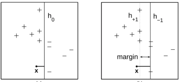
Fig. 1.Two equivalent ways to apply the SVMs classification rule. In Panel (a), the test pointxreceives the label (+1) assigned using hyperplaneh0,
Pl
i=1yiαiκ(xi,x)+b= 0. In Panel (b), the same test point receives the label (+1) assigned using the farthest away semi-consistent hyperplane from it (h−1,
Pl
i=1yiαiκ(xi,x) +b=−1), which is parallel to another semi-consistent hyperplane (h+1,
Pl
i=1yiαiκ(xi,x) +b= 1) in such
a way that the distance between these two hyperplanes is maximal.
An advantage of the SHs method is that it is robust against outliers and avoids overfitting. Further, we demonstrate empirically that the SHs decision boundary appears to be relatively insensitive to the choice of kernel applied to the data. The SHs approach is more conservative than SVMs, for instance, in the sense that the hyperplane determining the classification of a new object is more distant from it than any of the hyperplanes forming the so-called margin in SVMs. It can be argued that the SHs approach is more general than SVMs by means of a formulation of the SHs decision boundary that is nested into the formulation of the SVMs decision boundary.
2
Support Vector Machines for Classification
We start with an account of the SVM classifier, developed by Vapnik ([11]) and co-workers. SVMs for binary classification solve the following task: given training data {xi, yi}l
i=1 from Rn× {−1,1}, estimate a function f :Rn → {−1,1} such
that f will classify correctly unseen observations {xj, yj}lj+1+=l+1m. In SVMs, the
input vectors {xi}l
i=1 are usually mapped from Rn into a higher-dimensional
space via a mapping ϕ, in which the vectors are denoted as {ϕ(xi)}l i=1. In
this higher-dimensional (or, feature) space, the SVM method finds the hyper-plane that maximizes the closest distance between the observations from the two classes, the so-called margin, while at the same time minimizes the amount of
training errors ([2], [4], [11]). The optimal SVM hyperplane is found by solving the following quadratic optimization problem:
max α Pl i=1αi−12 Pl i,j=1αiαjyiyjκ(xi,xj) (1) s.t. 0≤αi≤C, i= 1,2, . . . , l, and Pl i=1yiαi= 0,
where κ(xi,xj) = ϕ(xi)0ϕ(xj) is a Mercer kernel that calculates the inner
product of input vectors xi and xj mapped in feature space. Using the opti-mal α’s of (1) the SVM hyperplane h0, w0ϕ(x) +b = 0, can be expressed as
Pl
i=1yiαiκ(xi,x) +b = 0. Here,w is a vector of hyperplane coefficients, and
b is the intercept. A test observationx receives the class label assigned using h0, as shown in Fig. 1a. Stated equivalently, x is classified using the
farthest-away hyperplane that is semi-consistent with the training data, which is parallel to another semi-consistent hyperplane in such a way that the distance between these two hyperplanes is maximal (see Fig. 1b).
3
Support Hyperplanes
3.1 Definition and Motivation
Just like SVMs, the SHs address the classification task. Let us focus on the so-called linearly separable case, where the positive and negative observations of a training data set D are perfectly separable from each other by a hyperplane. Consider the set of semi-consistent hyperplanes. Formally, a hyperplane with equationw0x+b= 0 is defined to be semi-consistent with a given data set if for all
data pointsi= 1,2, . . . , l, it holds thatyi(w0xi+b)≥0; the same hyperplane is defined to be consistent with the data if for all data pointsi= 1,2, . . . , l, it holds thatyi(w0xi+b)>0. The basic motivation behind Support Hyperplanes (SHs) is the desire to classify a test observationxwith that semi-consistent hyperplane, which is in some sense the most likely to assign the correct label tox. The extent of such likeliness is assumed to be positively related to the distance between x and any semi-consistent hyperplane. Thus, ifxis more distant from hyperplane ha than from hyperplanehb, both of which are semi-consistent withD, thenha is considered more likely to classifyxcorrectly than hyperplanehb. This leads to the following classification rule of SHs: a test pointx should be classified using the farthest-away hyperplane from x that is semi-consistent with the training data. Intuitively, this hyperplane can be called the “support hyperplane” since it supports its own judgement about the classification of x with greatest self-confidence; hence the name Support Hyperplanes for the whole method. For each test point x the corresponding support hyperplane is different. Therefore, the entire decision boundary between the two classes is not explicitly computed. A point is defined to lie on the SHs decision boundary if there exist two different semi-consistent hyperplanes that are farthest away from it. SHs consider the distance between a test pointxand a semi-consistent hyperplane as a proxy for complexity associated with the classification of x. Under this circumstance, the
best generalizability is achieved when one classifiesxwith the so-called support hyperplane: the semi-consistent hyperplane that is most distant from x. If one however considers the width of the margin as a proxy for complexity, then the SVM hyperplane achieves the best generalizability. Notice that by definition the support hyperplane is at least as distant fromxas any of the two semi-consistent hyperplanes that form the margin of the optimal SVM hyperplane, which makes
(a) (b)
a
b
x x
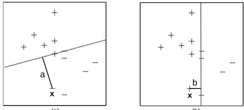
Fig. 2.Classification with Support Hyperplanes in two steps. At stage one (Panel (a)), a test pointx is added as class “–” to the original data set that consists of “+” and “–” labeled points, and the distance a from x to the farthest away semi-consistent hyperplane is computed. At stage two (Panel (b)),xis added to the original data set as class “+”, and the distancebfromxto the farthest away semi-consistent hyperplane is computed. Ifa > b(a < b), thenxis assigned to class “–” (“+”).
the SHs method relatively more conservative. Let us now argue more formally that the SH approach generalizes SVM by means of a formulation of the SHs decision boundary that is part of a formulation of the SVMs decision boundary. A pointxis defined to lie on the implicit SHs separation surface if the following three conditions are met: (1)xis equally distant from two hyperplanes, (2) these two hyperplanes are semi-consistent with the training data, and (3) the distance between pointxand any of the two hyperplanes is maximal. Next, observe that a pointxis defined to lie on the explicit SVMs optimal hyperplane if and only if the three conditions above plus an additional fourth condition are all satisfied: (4) the two (semi-consistent) hyperplanes are parallel to each other.
3.2 Estimation
Given a linearly separable data setD,{xi, yi}l
i=1, fromRn×{−1,1}, SHs classify
a test pointxl+1using that semi-consistent hyperplane with respect toD, which
is most distant from xl+1. Formally, in order to find the support hyperplane
w0x+b = 0 of point xl
problem: min w,b,yl+1 1 2w 0w (2) s.t. yi(w0xi+b)≥0, i= 1,2, . . . , l yl+1(w0xl+1+b) = 1
The distance between the support hyperplanew0x+b = 0 andxl
+1 is defined
as 1/√w0w by the last constraint of (2), irrespective of the label yl+1. This
distance is maximal when 1
2w0w is minimal. The role of the first l inequality
constraints is to ensure that the support hyperplane is semi-consistent with the training data.
Optimization problem (2) is partially combinatorial, since not all variables are continuous: the label yl+1 can take only two discrete values. Therefore, in
order to solve (2), two distinct optimization subproblems should we solved (see Fig. 2). One time (2) is solved when yl+1 equals +1, and another time when
yl+1 equals−1. Each of these optimization subproblems has a unique solution,
provided that the extended data set{xi, yi}li+1=1is separable. In case the two so-lutions yield the same value for the objective function 12w0w, the test pointxl
+1
lies on the SHs decision boundary and the classification label is undetermined. If the extended data set has become nonseparable whenyl+1is labeled, say, +1,
then the respective optimization subproblem does not have a solution. Then, xl+1 is assigned the opposite label, here −1. A way to detect whether a
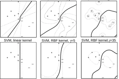
sub-problem has become nonseparable from separable will be described in [8]. The implicit nature of SHs provides for the property that the SHs decision boundary is in general nonlinear, even in case the original data is not mapped into a higher-dimensional space. Figure 3 demonstrates that this property does not hold in general for SVMs. This figure also illustrates that the SHs decision boundary appears to be less sensitive to the choice of kernel and kernel parameters than the respective SVMs boundary.
We now treat the so-called (linearly) nonseparable case. A training data set is said to be nonseparable if there does not exist a single hyperplane that is consistent with it. SHs deal with the nonseparable case in the same way as SVMs: by introducing so-called slack variables. For SHs, this procedure amounts to solving the following quadratic optimization problem:
min w,b,yl+1,ξ 1 2w 0w+C l X i=1 ξi (3) s.t. yi(w0xi+b)≥0−ξi, ξi ≥0, i= 1,2, . . . , l yl+1(w0xl+1+b) = 1.
Note that in (3) the points that are incorrectly classified are penalized linearly viaPli=1ξi. If one prefers a quadratic penalization of the classification errors, then the sum of squared errorsPli=1ξ2
i should be substituted for Pl
i=1ξiin (3). One can go even further and extend the SHs algorithm in a way analogical to
LS-SVM ([5]) by imposing in (3) that constraintsyi(w0xi+b)≥0−ξi hold as equalities, on top of substitutingPli=1ξ2
i for Pl
i=1ξi.
Each of the two primal subproblems pertaining to (3) can be expressed in dual form1as:
SH, linear kernel SVM, linear kernel SH, RBF kernel, γ=5 SVM, RBF kernel, γ=5 SH, RBF kernel,γ=35 SVM, RBF kernel,γ=35
Fig. 3.Decision boundaries for SHs and SVMs using the linear,κ(xi,xj) =x0ixj, and the RBF, κ(xi,xj) = exp(−γ kxi−xj k2), kernels on a linearly separable data set. The dashed contours for the SHs method are iso-curves along which the ratio of two distances is constant: the distance from a test point to the farthest semi-consistent hyperplane when it is added to the data set one time as “+”, and another time as “–”.
max α αl+1− 1 2 Pl+1 i,j=1αiαjyiyj(x0ixj) (4) s.t. 0≤αi≤C, i= 1,2, . . . , l, and Pl+1 i=1yiαi= 0,
where theα’s are the Lagrange multipliers associated with the respective sub-problem. In the first subproblem yl+1 = 1, while in the second subproblem
yl+1 =−1. The advantage of the dual formulation (4) is that different Mercer
kernels can be employed to replace the inner productx0
ixj in (4), just like in the SVMs case. The (l+1)×(l+1) symmetric positive-definite matrix with elements ϕ(xi)0ϕ(xj) on theithrow andjthcolumn is called the kernel matrix.
The SHs approach can also be theoretically justified by observing that a kernel matrix used by SHs can be modified to represent the original SHs opti-mization problem as an SVM problem. It turns out that the theoretical under-pinnings for SVMs can also be transferred to the SHs method. More details will be provided in [8].
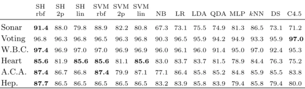
Table 1.Leave-one-out accuracy rates (in %) of the Support Hyperplanes classifier as well as some standard methods on several binary data sets. Rbf, 2p and lin stand for Radial Basis Function, second-degree polynomial and linear kernel, respectively
SH SH SH SVM SVM SVM
rbf 2p lin rbf 2p lin NB LR LDA QDA MLP kNN DS C4.5 Sonar 91.4 88.0 79.8 88.9 82.2 80.8 67.3 73.1 75.5 74.9 81.3 86.5 73.1 71.2 Voting 96.8 96.3 96.8 96.5 96.3 96.8 90.3 96.5 95.9 94.2 94.9 93.3 95.9 97.0 W.B.C. 97.4 96.9 97.0 97.0 96.9 96.9 96.0 96.1 96.0 91.4 95.0 97.0 92.4 95.3 Heart 85.6 81.9 85.6 85.6 81.1 85.6 83.0 83.7 83.7 81.5 78.9 84.4 76.3 75.2 A.C.A. 87.4 86.7 86.8 87.4 79.9 87.1 77.1 86.4 85.8 85.2 84.8 85.9 85.5 83.8 Hep. 87.7 86.5 86.5 86.5 86.5 86.5 83.2 83.9 85.8 83.9 79.4 85.8 79.4 80.0
4
Experiments on Some UCI and SlatLog Data Sets
The basic optimization algorithm for Support Hyperplanes (4) is implemented via a modification of the freely available LIBSVM software ([3]). We tested the performance of Support Hyperplanes on several small- to middle-sized binary data sets that are freely available from the SlatLog and UCI repositories ([9]) and have been analyzed by many researchers and practitioners (e.g. [1], [6], [7], [10] and others):Sonar,Voting,Wisconsin Breast Cancer (W.B.C.),Heart, Australian Credit Approval (A.C.A.), andHepatitis(Hep.). Detailed information on these data sets can be found on the web sites of the respective repositories.
We compare the results of SHs to those of several state-of-art techniques: Linear and Quadratic Discriminant Analysis (LDA and QDA), Logistic Regres-sion (LR), Multi-layer Perceptron (MLP), k-Nearest Neighbor (kNN), Naive Bayes classifier (NB) and two types of Decision Trees – Decision Stump (DS) and C4.5. The experiments for the NB, LR, MLP, kNN, DS and C4.5 meth-ods have been carried out with the WEKA learning environment using default model parameters, except forkNN. We refer to [12] for additional information on these classifiers and their implementation. We measure model performance by the leave-one-out (LOO) accuracy rate. For our purposes – comparison between the methods – LOO seems to be more suitable than the more general k-fold cross-validation (CV), because it always yields one and the same error rate es-timate for a given model, unlike the CV method (which involves a random split of the data into several parts).
Table 1 presents performance results for all methods considered. Some meth-ods, namelykNN, SHs and SVMs, require tuning of model parameters. In these cases, we report only the highest LOO accuracy rate obtained by performing a grid search for tuning the necessary parameters. Overall, the accuracy rates of Support Hyperplanes exhibit first-rate performance on all six data sets: five times out of six the accuracy rate of SHs is the highest one. SVMs follow closely, and the rest of the techniques show relatively less favorable and more volatile results. For example, the C4.5 classifier performs best on the Voting data set,
but achieves rather low accuracy rates on two other data sets –SonarandHeart. Note that not all data sets are equally easy to handle. For instance, the perfor-mance variation over all classifiers on theVoting andBreast Cancer data sets is rather low, whereas on theSonar data set it is quite substantial.
5
Conclusion
We have introduced a new technique that can be considered as a type of an instance-based large margin classifier, called Support Hyperplanes (SHs). SHs induce an implicit and generally nonlinear decision surface between the classes by using a set of (explicitly defined) hyperplanes. SHs classify a test observation using the farthest-away hyperplane from it that is semi-consistent with the data used for training. This results in a good generalization quality. Although we have treated just the binary case, the multi-class extension can easily be carried out by means of standard methods such as one-against-one or one-against-all classification. A potential weak point of SHs, also applying to SVMs, is that it is not clear a priori which type of kernel and what value of the tuning parameters should be used. Furthermore, we do not address the issue of attribute selection and the estimation of class-membership probabilities. Further research could also concentrate on the application of SHs in more domains, on faster implementation suitable for analyzing large-scale data sets, and on the derivation of theoretical test-error bounds.
References
1. Breiman, L.: Bagging predictors. Machine Learning24(1996) 123–140
2. Burges, C.: A tutorial on support vector machines for pattern recognition. Data Mining and Knowledge Discovery2(1998) 121–167
3. Chang, C.C., Lin, C.J.: LIBSVM: a library for support vector machines (2006) Software available athttp://www.csie.ntu.edu.tw/∼cjlin/libsvm.
4. Cristianini, N., Shawe-Taylor, J.: An Introduction to Support Vector Machines. Cambridge University Press (2000)
5. van Gestel, T.V., Suykens, J.A.K., Baesens, B., Viaene, S., Vanthienen, J., De-dene, G., Moor, B.D., Vandewalle, J.: Benchmarking least squares support vector machine classifiers. Machine Learning 24(2004) 5–32
6. King, R.D., Feng, C., Sutherland, A.: STATLOG: comparison of classification al-gorithms on large real-world problems. Applied Artificial Intelligence 9(3)(1995) 289–334
7. Lim, T., Loh, W., Shih, Y.: A comparison of prediction accuracy, complexity, and training time for thirtythree old and new classification algorithms. Machine Learning40(1995) 203–228
8. Nalbantov, G.I., Bioch, J.C., Groenen, P.J.F.: Instance-based classification with support hyperplanes. Econometric Institute technical report, Erasmus University Rottedam (to appear)
9. Newman, D., Hettich, S., Blake, C., Merz, C.: UCI Repository of machine learning databases (1998)http://www.ics.uci.edu/∼mlearn/MLRepository.html Univer-sity of California, Irvine, Dept. of Information and Computer Sciences.
10. Perlich, C., Provost, F., Simonoff, J.S.: Tree induction vs. logistic regression: a learning-curve analysis. Journal Of Machine Learning Research4(2003) 211–255 11. Vapnik, V.N.: The Nature of Statistical Learning Theory. Springer-Verlag New
York, Inc. (1995) 2nd edition, 2000.
12. Witten, I.H., Frank, E.: Data Mining: Practical machine learning tools and tech-niques. Morgan Kaufman, San Francisco (2005) 2nd edition.