© 2014 Museu de Ciències Naturals de Barcelona ISSN: 1578–665 X
eISSN: 2014–928 X
Sarmento, P., Cruz, J., Eira, C. & Fonseca, C., 2014. A spatially explicit approach for estimating space use and density of common genets. Animal Biodiversity and Conservation, 37.1: 23–33.
Abstract
A spatially explicit approach for estimating space use and density of common genets.— Many species that occur at low densities are not accurately estimated using capture–recapture methods as such techniques assume that populations are well–defined in space. To solve this bias, spatially explicit capture–recapture (SECR) models have recently been developed. These models incorporate movement and can identify areas where it is more likely for individuals to concentrate their activity. In this study, we used data from camera–trap surveys of common genets (Genetta genetta) in Serra da Malcata (Portugal), designed to compare abundance estimates produced by SECR models with traditional closed–capture models. Using the SECR models, we observed spatial heterogeneity in genet distribution and density estimates were approximately two times lower than those obtained from the closed popula� tion models. The non–spatial model estimates were constrained to sampling grid size and likely underestimated movements, thereby overestimating density. Future research should consider the incorporation of cost–weighed models that can include explicit hypothesis on how environmental variables influence the distance metric. Key words: Camera–trapping, Capture–recapture, Genet, Program MARK, SECR package, Spatial models. Resumen
Un método espacialmente explícito para estimar el uso del espacio y la densidad de la jineta común.— Muchas especies con baja densidad de población no se estiman con precisión utilizando métodos de captura y recaptura, puesto que tales técnicas suponen que las poblaciones están bien definidas en el espacio. Para resolver este sesgo, recientemente se han elaborado modelos de captura y recaptura espacialmente explícitos (SECR). Estos modelos incorporan el movimiento y pueden determinar las zonas en la que es más probable que los individuos concentren su actividad. En el presente estudio, utilizamos datos obtenidos con cámaras de trampeo en estudios sobre la jineta común (Genetta genetta) en Serra da Malcata (Portugal) concebidos para comparar las estimaciones de abundancia producidas por los modelos de SECR y los modelos tradicionales de captura para una población cerrada. Utilizando los modelos de SECR, observamos la existencia de heterogeneidad espacial en la distribución de la jineta y las estimaciones de la densidad fueron aproximadamente dos veces inferiores a las obtenidas en los modelos para poblaciones cerradas. Las estimaciones del modelo no espacial se limitaron al tamaño de la cuadrícula de muestreo y probablemente infravaloraron los movimientos, lo que conllevaría que se sobreestimara la densidad. Los estudios futuros deberían sopesar la incorporación de modelos de carga–distancia que puedan incluir hipótesis explícitas sobre la forma en que las variables medioambientales influyen en la métrica de la distancia.
Palabras clave: Trampeo con cámara, Captura y recaptura, Jineta, Programa MARK, Paquete de SECR, Modelos espaciales.
Received: 27 VIII 13; Conditional acceptance: 20 XI 13; Final acceptance: 12 III 14
Pedro Sarmento, Catarina Eira & Carlos Fonseca, Center for Environmental and Marine Studies and Biology Dept., Aveiro Univ., Campus Universitário de Santiago, 3810–193 Aveiro, Portugal.– Joana Cruz, Environment Dept., Univ. of York, YO10 5DD, United Kingdom.
Corresponding author: P. Sarmento. E–mail: [email protected]
A spatially explicit approach for
estimating space use and density of
common genets
Introduction
Researchers seeking to understand population proc� esses need methods and models that provide accurate inferences on population status. Camera trap methods have proven to be very useful to study animals that live in areas that are too large to study as a whole, and ani� mals that are elusive and difficult to observe (Gardner et al., 2010a). Many of the wide ranging species studied with camera traps methods occur at low densities. In such species, the conventional capture–recapture (CR) theory to this species is likely unsatisfactory as it is more suited to high density species occurring over relatively small ranges (Foster & Harmsen, 2012). The main problems when dealing with wide–ranging and/or elusive species are the relatively small sample sizes, low capture probabilities, and the effects of individual heterogeneity (Royle et al., 2011a). The usual method to analyse density is to apply closed population mod� els (White & Burnham, 1999), and convert these to densities using fundamentally ad hoc methods (Trolle et al., 2007). This approach presents two important difficulties: (1) the assumption of geographic closure of the population, i.e., no movement in and out of the sampling grid (White et al., 1982) which is frequently violated (Karanth & Nichols, 1998), and (2) the difficulty of estimating the effective sampling area (Balme et al., 2009a). The typical methodology consists of generating a buffer around the grid with half the mean maximum linear distance moved by animals captured in more than one trap (1/2MMDM) (Karanth & Nichols, 1998). Other approaches to estimate the buffer width include the full MMDM (Trolle et al., 2007), and the radius of an average home range (Sarmento et al., 2009).These approaches also present major problems: (1) They lack theoretical justification, being mostly ad hoc methods (Bochers & Efford, 2008); and (2)comparisons of es� timates from different methodologiesbecome difficult (Sollmann et al., 2011).
Furthermore, conventional CR methods assume that populations are well–defined in the sense that one can randomly sample individuals associated with a defined study location or area (Royle et al., 2009). However, individuals within populations are spatially organized and during the trapping periods they can display move� ment patterns that increase or decrease their capture probability (Gardner et al., 2010b; Sollmann et al., 2011). Relating their movement patterns to the trapping grid therefore has important implications for sampling design, modelling, and interpretation of data (Foster & Harmsen, 2012). The problem with classical closed population models for estimating density from trapping arrays is that 'space' has no explicit manifestation. This dilemma is solved with the recently developed spatially explicit capture–recapture models (SECR), which in�(SECR), which in�), which in� corporate movement by assuming that each individual i has an activity centre si, which remains constant over the survey, and that the capture probability in a trap j is a monotonically decreasing function of the distance between the activity centre and trap j (Borchers & Ef� ford, 2008). Using these models we can also obtain maps of density of activity centres, which correspond to areas where it is more likely that individuals concentrate
their activity. For camera trapping studies, the Poisson model is usually used (Borchers & Efford, 2008). This model assumes that an individual can be captured an arbitrary number of times in an arbitrary number of traps (Borchers & Efford, 2008). Model parameters can include: (1) the baseline trap encounter rate (λ0), which is defined as the expected number of detections of the individual i in a hypothetical trap located at the activity centre (Royle et al., 2009); (2) the movement parameter (σ), which controls the shape of the distance function, being expressed in the same unit used for the trapping grid (km); this parameter can be converted to a 95% home range radius by assuming a circular bivariate normal model for movement; and (3) density (D), is calculated by dividing N by the area of the state space (S), which is user–defined, includes the trapping grid (Borchers & Efford, 2008), and needs to be large enough to contain all individuals potentially exposed to the grid.
SECR models can be implemented in several soft�can be implemented in several soft� ware packages: DENSITY (Efford, 2008), SECR pack� age (Efford, 2011) in program R, version 2.10.1 (R, 2006), and SPACECAP (Gopalaswamy et al., 2012). These platforms differ in their statistical paradigms: (1) likelihood based classical inference (DENSITY and SECR) and (2) Bayesian inference (SPACECAP). Integrated likelihood is an adequate process for analyzing these models, since they are created in terms of a set of latent variables or random effects that corre� spond to individual locations (Borchers & Efford, 2008). The observation model is conceptualized conditionally on the random effects, and inference is formally based on the likelihood created from the marginal probability distribution of the observations (Bochers & Efford, 2008). The random effects are eliminated from the conditional likelihood by integration, which is achieved numerically in SECR models.
In this paper we used data collected during three camera–trapping surveys designed for common genets (Genetta genetta) in Serra da Malcata (Portugal) (Sarmento et al., 2010) to compare density estimates produced by SECR models with traditional closed capture models generated by program MARK (White & Burnham, 1999). We tested several models that incorporate habitat and heterogeneity effects and we discuss the major differences and potential advantages of each statistical framework. Common genets are an important forest species, and their density can be used as an indicator of ecosystem fitness, particularly in hu� man altered landscapes and protected areas (Sarmento et al., 2010). The development of suitable methods to evaluate the abundance of this species can therefore be of great importance.
Materials and methods Study area
The Serra da Malcata (fig. 1) is a Mediterranean moun� tainous area of 200–km2 located in Portugal close to the Spanish border (40º 08' 50'' N – 40º 19' 40'' N and 6º 54' 10'' W – 7º 09' 14'' W). Vegetation is dominated
by dense scrublands of Cytisus spp., Halimium spp., Cistus spp., Erica spp., Chamaespartium tridentatum and Arbutus unedo covering 43% of the area. Scattered woodlands of Quercus rotundifolia and Q. pyrenaica trees compose 15% of Serra da Malcata. Thirty percent (30%) of the area is covered by plantations of Pinus spp., Eucalyptus globulus and Pseudotsuga menziesii and the remaining 12% is cropland. Around 60% of Serra da Malcata is a protected area included in Serra da Malcata Nature Reserve.
Camera–trapping
We studied the distribution and abundance of common genets from October 2005 to November 2007. We used four different camera devices: (1) CamTracker® analogical system; (2) DeerCam® analogical system (DeerCam – Scouting Camera, Non Typical Inc., USA); (3) Bushnell trophy cam® digital camera (Bushnell Corp., Overland Park, KS, USA); and (4) GameSpy® digital camera (EBSCO Industries, Inc., East Birming� ham, AL, USA). The cameras were positioned 20 cm (average) above ground and distanced 2 to 4 m from the lure, which consisted of domestic cat urine sprayed on a piece of cork–tree bark connected to a wooden stake at a 40–50 cm height (Sarmento et al., 2009).
Trap–stations were placed in a trapping grid arrange� ment where the distance between cameras should be, at most, the diameter of a circle encompassing the smallest home–range described for the target species in the study area (Sarmento et al., 2010). Therefore, cameras were placed at a distance of 300 to 500 m, according to Cruz (Cruz, 2002). We divided the study into three trapping surveys (table 1), which were divided in an average of seven capture occasions of seven days (Karanth & Nichols, 1998). Genets were individually identified based on their distinct pelage patterns (Sarmento et al., 2010). Spatially explicit models
Spatially explicit models combine a state model and an observation model (Borchers & Efford, 2008). The state model expresses the geographic distribution of individual home ranges, while the observation or spatial detection model estimates the probability of detecting an individual at a given detector (e.g. camera trap) to the distance of this detector from a central point in every animal’s home range (Borchers & Efford, 2008). The distribution of range centres in the population can be treated as a homogeneous Poisson point process. We estimated genet density by using the likelihood based classical inference in SECR package.
SM02 SM01 SM03 Portugal Spain N W E S Camera traps Serra de Malcata Nature Reserve Portugal 0 750 1,500 3,000 4,500 6,000 m
Fig. 1. Geographic location of the three trapping campaigns for common genets in Serra da Malcata Nature Reserve, Portugal, 2005–2007. The buffer around the camera–traps corresponds to the 1/2MMDM distance. Fig. 1. Localización geográfica de las tres campañas de trampeo de la jineta común en la reserva natural de Serra da Malcata (Portugal), entre 2005 y 2007. El área de influencia alrededor de las cámaras de trampeo equivale a un 1/2MMDM de la distancia.
The SECR package uses SECR models based on the maximum likelihood approach (ML SECR) (Efford, 2011). One important step when using this package is to define the detector type. Since camera traps do not capture animals but simply record their passage we use a detector type called 'proximity'. These 'proximity' detectors can be considered to act independently of each other and may catch more than one animal at a time (Efford et al., 2009). Input data is expressed in two files: (1) one that contains the name and geographic coordinates of the detec� tors (cameras); (2) another containing the capture histories, which include season, animal identification, the occasion, and the detector.
Considering that we want to model the detection probability of each individual i on occasion s at detector k, and considering we have observed n individuals on S occasions at K detectors, we will have n*S*K detection probabilities. In this framework a null model assumes that all n*S*K detection probabilities are the same. The usual sources of variation in capture probability can emerge in the n dimension as individual heterogeneity (corresponds to the Mh model), in the S dimension (corresponds to the Mt model of time variation) or as a particular interaction in these two dimensions (as a behavioural response to capture, corresponding to a Mb model). In these models, therefore, the detection probability can have two parameters (e.g. λ0, б for a half–normal function), or three parameters (e.g. λ0, б, z). These parameters may vary with respect to individual (i), occasion (s), or detector (k). Considering these specifications, we defined six models (Efford, 2011): (1) a null model with the notation 'λ0 ~ 1', where λ0 is constant across animals, occasions and detectors; (2) a behaviour model with the notation 'λ0 ~ b', where λ0 is affected by a reaction of the individuals to traps; (3) a model with learned response that affects both λ0 and б with the notation 'list (λ0 ~ b,б ~ b)'; (4) a heterogeneity model with a 2–class finite mixture for λ0 noted as 'λ0 ~ h2'; (5) a time variation model with the notation 'λ0 ~ T'; and (6) a learned response model in λ0 combined with trend over occasions noted as 'λ0 ~ b + T'.
Candidate models were ranked using the Akaike Information Criterion corrected for small samples sizes (AICc) by calculating their Akaike weights (Burnham & Anderson, 2002). Models with ΔAICc values ≤ 2 from the most parsimonious model were considered strongly supported. Akaike weights (ω) were used to further interpret the relative importance of each model´s independent variable. ΔAICc values were used to compute ωi, which is the weight of evidence in favour of a model being the best approximating model given the model set (Burnham & Anderson, 2002). Unless a single model had a ωi > 0.9, other models were con� sidered when drawing inferences about the data, by calculating the averaged parameters using ω values (Burnham & Anderson, 2002).
Population closure was estimated using the sta� tistical test of Stanley & Richards (2005). Finally, we computed the probability density of home range centres of detected animals (Borchers & Efford, 2008) for the best ranked model by using the function 'fxi'.
Capture–recapture non–spatial model
Genet abundance under a non–spatial scenario was estimated using the model 'full closed captures with heterogeneity' available in program MARK (White & Burnham, 1999). These models include a finite mixture as an estimate of individual heterogeneity in capture probability. The finite mixture is character� ized by a parameter π, which is the probability of an individual belonging to mixture a, for one or more mixtures. These models allow capture probability (p) and recapture probability (c) to vary with time or as a behaviour response to traps. Model selection was performed using Akaike’s information criterion (AICc) corrected for small sample size (Burnham & Anderson, 2002) as described above. The effective sampled area was determined using the 1/2MMDM (fig. 1) to generate a buffer around the trapping polygon (Balme et al., 2009a). Density was estimated by dividing N (obtained from the best ranking model) by this area. We evaluated the likelihood of population closure using the Close Test Program (Stanley & Richards, 2005). Each trapping campaign corresponded to 7–day sampling occasions to generate a sufficient number of captures, thereby maximizing the number of sampling occasions without violating population closure assumptions.
Results Genet captures
From 2005 to 2007, we obtained a capture success of 2.44 captures/100 trap–nights (table 1), which equals 1 genet capture for every 40.98 nights of trapping. Genets were photographed in 41% of tra� pping stations (n = 34). On average, we obtained 0.68 (SE = 0.14) captures per trap (min = 0; max = 5). Falsely triggered images constituted 36.19% of all images and were mostly caused by rain, wind and extreme heat.
Spatially explicit models
For trapping survey SM01 closed test results indicated that the population was closed to gains and losses during the trapping period (z = –0.08; p = 0.46). Only the null model had ΔAICc ≤ 2 with ωi = 0.95 (table 2), indicating no effects of time, behaviour or heterogeneity in the parameters of the models. We estimated a sampling area of 64.99 km2 (table 3). The baseline encounter rate (λ0), estimated at 0.22 (table 3), reached the asymptotic zero at a distance of approximately 2,000 m, indicating that an animal whose activity centre was located at this distance from a given trap had a theoretical capture probability of zero (the probability of being detected in that trap was zero) (fig. 2). Considering the contours of the net probability of detection, we observed that animals with an activity centre within a buffer of 250 m around the trapping polygon had a 0.99 probability of being
caught in any trap (fig. 3). For this model, we esti� mated a genet density of 0.30 (95% CI, 0.61–0.42), corresponding to an average estimated population of 20 individuals (95% CI, 11–27) (table 3).
The premise of population closure was observed for trapping campaign SM02 (z = –0.103; p = 0.151). For this campaign we obtained 2 models with a ∆AICc < 2 (table 2). Therefore, no single model emerged as the top ranking model, i.e. ωi > 0.90. The model with the greatest support was SECR–T, followed by SECR–0 (table 2), suggesting that capture probability could be time dependent. The application of a LR test revealed no significant differences between the two models (
x
12 = 0.94; p = 0.75), so the averaged model was used to calculate the final parameters. An averaged value of 0.13 (CI 95% = 0.06–0.25) was obtained for λ0 (table 3).The estimated detection probability was 0 at an aver� aged distance of 1,800 m from the traps (fig. 2). Using this model we estimated a genet density of 0.39/km2 (95% CI, 0.19–0.79). corresponding to an estimated population of 23 individuals (95% CI, 11–47) (table 4). We also observed population closure during the SM03 trapping campaign (z = –0.275; p = 0.392). The null model (SECR–0) emerged as the most robust, being the only model with ∆AICc < 2, closely followed by the behaviour model (SECR–b) (table 2). Considering this proximity and the results of an LR test, which revealed no significant differences between the two models (
x
12 = 0.98; p = 0.75), we used the averaged model to calculate the final parameters. The detection probability decreased consistently with increasing distance from the trapping polygon, presenting an estimated value of 0 at Table 1. Camera trapping periods and sampling effort during three trapping campaigns in Serra da Malcata Nature Reserve, Portugal, 2005–2007.Tabla 1. Períodos de trampeo con cámara y esfuerzo de muestro durante tres campañas de muestreo llevadas a cabo en la reserva natural de Serra da Malcata, Portugal, entre 2005 y 2007.
Area Sampling period Trap stations Camera–days Photos Captures Individuals
SM01 10 X–6 XII 2005 29 1,653 25 17 9
SM02 6 X–20 XI 2006 30 1,350 27 21 10
SM03 14 X–19 XI 2007 23 828 29 19 9
Total 82 2,331 81 57 28
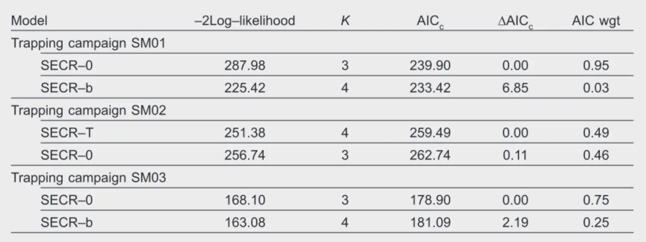
Table 2. Best two ranked models of a model selection analysis (ΔAIC < 2) of spatially explicit capture– recapture models for genets obtained during three camera–trapping campaigns in Serra da Malcata Nature Reserve, Portugal, 2005–2007.
Tabla 2. Los dos modelos mejor clasificados en un análisis de selección (ΔAIC < 2) de modelos de captura y recaptura espacialmente explícitos para la jineta obtenidos durante tres campañas de muestreo con cámaras llevadas a cabo en la reserva natural de Serra da Malcata, Portugal), entre 2005 y 2007.
Model –2Log–likelihood K AICc ∆AICc AIC wgt
Trapping campaign SM01 SECR–0 287.98 3 239.90 0.00 0.95 SECR–b 225.42 4 233.42 6.85 0.03 Trapping campaign SM02 SECR–T 251.38 4 259.49 0.00 0.49 SECR–0 256.74 3 262.74 0.11 0.46 Trapping campaign SM03 SECR–0 168.10 3 178.90 0.00 0.75 SECR–b 163.08 4 181.09 2.19 0.25
an averaged distance of 2,000 m (fig. 2). An averaged density of genets was estimated at 0.18 individuals/km2 (95% CI, 0.19–0.79), corresponding to an estimated population of 21 individuals (95% CI, 11–42) (table 4). Closed capture–recapture models
For all the trapping campaigns in the best–ranked models, p and c did not vary with time and were different (i.e. they showed a behaviour response to traps) (table 4). The recapture probability was always lower than p, which reflects a negative effect of the traps after the first capture. Average capture proba� bility was estimated at 0.61 (95% CI = 0.37–0.78), and the average recapture probability was 0.40 (95% CI = 0.26–0.52) (table 5). Density values varied bet� ween 0.45 and 0.73 individual/km2, with an average of 0.61 (95% CI = 0.58–0.67) (table 5).
Discussion
Over the last 10 years, camera trapping has become one of the most useful tools to estimate animal abun� dance, particularly in species that can be individually identified (Balme et al., 2009b; Negrões et al., 2010;
Sarmento et al., 2010). The most common approach is to combine this technique with standard closed population models. The theoretical constraint of closed population estimators is that, although abundance estimates may be suitable to calculate the numbers of a population that are exposed to traps, individual movements cannot be precisely associated to an accurate area (Royle et al., 2011b). At the same time, closed population models cannot incorporate moving traps, open systems, or multiple captures in a single occasion.
The recent development of SECR models was crucial to deal with the baseline problem of abundance interpretation resulting from the ad–hoc approaches to estimate the sampling area in non–spatial capture– recapture models (Borchers & Efford, 2008). Using the classic estimation of abundance, it is difficult to compare different areas. However, the flexibility of SECR models allows this comparison and also in� models allows this comparison and also in� cludes other aspects such as capture heterogeneity and covariate effects on capture probabilities (Borch� ers & Efford, 2008). The inclusion of trap–specific encounter histories in SECR models overcomes the problem of non–spatial models ignoring trap identity. In these models, if an animal is captured multiple times during a trapping period, these will count as
Table 3. Parameters estimates of spatially explicit capture–recapture models for genets obtained during three camera–trapping campaigns in Serra da Malcata Nature Reserve, Portugal, 2005–2007: S area. Effective sampled area (km2); λ
0. Baseline encounter rate / occasion; б. Movement parameter (m); D. Genet density (genets / km2); N. Number of genets in the sampled area.
Tabla 3. Estimaciones de los parámetros de los modelos de captura y recaptura espacialmente explícitos para la jineta obtenidas durante tres campañas de muestreo con cámaras llevadas a cabo en la reserva natural de Serra da Malcata, Portugal, entre 2005 y 2007: S area. Superficie efectiva muestreada (km2); λ0. Índice de referencia de encuentros / ocasión; б. Parámetro de movimiento (m); D. Densidad de la jineta (jinetas / km2); N. Número de jinetas en la zona muestreada.
Campaign Model S area λ0 б D N
SM01 SECR–0 64.99 0.22 759 0.30 20 (0.12–0.36) (540–1066) (0.16–0.42) (11–27) SM02 SECR–T 58.76 0.17 573 0.38 22 (0.07–0.34) (392–837) (0.18–0.76) (11–45) SECR–0 0.08 567 0.41 24 (0.04–0.16) (420–1667) (0.20–0.83) (12–49) Model 0.13 570 0.39 23 averaged (0.06–0.25) (405–1239) (0.19–0.79) (11–47) SM03 SECR–0 81.12 0.16 737 0.16 22 (0.07–0.34) (501–1084) (0.07–0.32) (11–45) SECR–b 0.49 742 0.19 15 (0.12–0.87) (503–1093) (0.09–0.42) (8–34) Model 0.24 738 0.18 21 averaged (0.14–0.46) (502–1086) (0.08–0.35) (11–42)
a single capture only, possibly leading to oss of information. Furthermore, in non–spatial models it is difficult to include different periods of individual trap activity (i.e. traps that were not always active during the entire trapping period) (Efford et al., 2013), which is not necessary in SECR models because they are based on trap–level encounters of individuals (Royle et al., 2011b).
SECR models assume the demographic closure of the population (i.e. no births, deaths, emigration or immigration during the study period). This popu� lation closure is assumed in the fixed nature of the estimated activity centres, which are considered to be constant over the trapping period. In this case, the presence of transient animals can be a factor of
population closure violation. According to Royle et al. (2011b) this non–closure can be overcome by model� this non–closure can be overcome by model� ling an individual–specific encounter probability scale parameter, σ, that incorporates individual variability in home–range size. More extensions to these models are currently being developed to include moving activ� ity centres. Such centres will be crucial in multi–year studies, since home–ranges can vary with changes in resource availability and in other biological aspects (Royle et al., 2009).
The density estimates obtained using the non–spa� tial model were, on average, 2.15 times higher than those obtained using the spatial model. This findings was also observed by other authors who performed the same type of comparison with Andean cats (
Leop-Fig. 2. Variation of the detection probability as a function of distance from an individual trap for three trapping surveys for common genets in Serra da Malcata Nature Reserve, Portugal, 2005–2007. Fig. 2. Variación de la probabilidad de detección en función de la distancia desde una cámara determinada para tres estudios de trampeo de la jineta común en la reserva natural de Serra da Malcata, Portugal, entre 2005 y 2007. SM01 SM02 SM03 0.25 0.20 0.15 0.10 0.05 0.00 0.10 0.08 0.06 0.04 0.02 0.00 0.20 0.15 0.10 0.05 0.00 0 500 1,000 1,500 2,000 2,500 3,000 0 1,000 2,000 3,000 4,000 5,000 Distance (m) Distance (m) 0 1,000 2,000 3,000 4,000 5,000 Distance (m) Detection pr oba bility Detection pr oba bility Detection pr oba bility
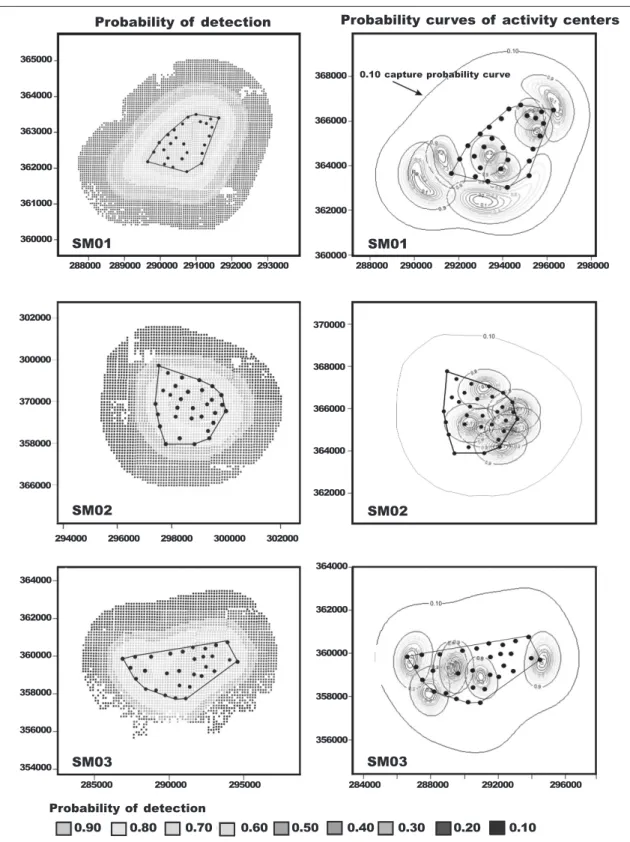
Fig. 3. Geographic distribution of the probability of detection around the trapping polygon for each potential home–range center (left column) and curves of probability of distribution of home range centers of animals that were detected for the three trapping campaigns (right column) for common genets in Serra da Malcata Nature Reserve, Portugal, 2005–2007.
Fig. 3. Distribución geográfica de la probabilidad de detección alrededor del polígono de trampeo para cada posible centro de área de distribución (columna izquierda) y curvas de probabilidad de la distribu-ción de dichos centros para los animales que se detectaron en las tres campañas de trampeo (columna derecha) de la jineta común en la reserva natural de Serra da Malcata, Portugal, entre 2005 y 2007.
SM01 SM01
SM02 SM02
SM03 SM03
Probability of detection Probability curves of activity centers
288000 289000 290000 291000 292000 293000 288000 290000 292000 294000 296000 298000 294000 296000 298000 300000 302000 285000 290000 295000 284000 288000 292000 296000 364000 362000 360000 358000 356000 354000 302000 300000 370000 358000 366000 365000 364000 363000 362000 361000 360000 368000 366000 364000 362000 360000 370000 368000 366000 364000 362000 364000 362000 360000 358000 356000
0.10 capture probability curve
Probability of detection
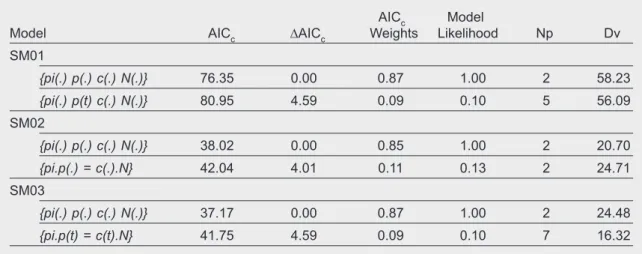
Table 4. Model selection statistics for the two best ranking models of full closed captures analysis on common genet capture–recapture data from Malcata, Portugal, 2005–2007: Np. Number of parameters; Dv. Deviance; pi. Probability of mixture; p. Capture probability; c. Recapture probability; N. Population size. The parameters p and c were modeled such as could be constant over sampling occasions (.) or varying with time (t).
Tabla 4. Valores de los criterios estadísticos para seleccionar modelos relativos a los dos mejores modelos de análisis de capturas en poblaciones totalmente cerradas aplicados a los datos obtenidos con la captura y recaptura de la jineta común en Malcata, Portugal, entre 2005 y 2007: Np. Número de parámetros; Dv. Desviación; pi. Probabilidad de mezcla; p. Probabilidad de captura; c. Probabilidad de recaptura; N. Tamaño de la población. Los parámetros p y c se utilizaron en el modelo como si pudieran ser constantes durante todas las ocasiones de muestreo (.) o variables con el tiempo (t).
AICc Model
Model AICc ∆AICc Weights Likelihood Np Dv
SM01 {pi(.) p(.) c(.) N(.)} 76.35 0.00 0.87 1.00 2 58.23 {pi(.) p(t) c(.) N(.)} 80.95 4.59 0.09 0.10 5 56.09 SM02 {pi(.) p(.) c(.) N(.)} 38.02 0.00 0.85 1.00 2 20.70 {pi.p(.) = c(.).N} 42.04 4.01 0.11 0.13 2 24.71 SM03 {pi(.) p(.) c(.) N(.)} 37.17 0.00 0.87 1.00 2 24.48 {pi.p(t) = c(t).N} 41.75 4.59 0.09 0.10 7 16.32
Table 5. Results of population closure, probability of mixture (π), capture (p) and recapture (c) probabilities and estimated abundance (N) and density (individuals / km2 [D]) of genet samples in Serra da Malcata Nature Reserve, Portugal, 2005–2007, using the best ranked model for each trapping campaign of table 4. Tabla 5. Resultados del grado en qué una población pueda ser considerada cerrada, la probabilidad de mezcla (π), las probabilidades de captura (p) y de recaptura (c) y la abundancia (N) y densidad (individuos / km2 [D]) estimadas a partir de las poblaciones de jineta estudiadas en la reserva natural de Serra da Malcata, Portugal, entre 2005 y 2007, utilizando el modelo mejor clasificado para cada campaña de trampeo de la tabla 4.
1/2MMDM area π p c N D (km2) SM01 0.47 0.60 0.42 10 0.59 16.88 (0.44–0.50) (0.34–0.80) (0.30–0.55) (9–11) (0.53–0.61) SM02 0.47 0.63 0.32 11 0.74 14.96 (0.30–0.63) (0.37–0.82) (0.18–0.49) (10–12) (0.67–0.80) SM03 0.48 0.75 0.42 9 0.46 19.74 (0.31–65) (0.45–0.91) (0.27–0.58) (9–10) (0.45–0.50)
ardus jacobita) (Reppucci et al., 2011) and jaguars
(Panthera onca) (Sollmann et al., 2011).
In conclusion, the use of SECR models overcomes several problems that can arise when estimating
density of genets or other cryptic, low–density spe� cies (Sollmann et al., 2011). One of the main advan� tages of these models is that they can be applied to any capture–recapture technique that is based on
individual identification and trap–specific encounter histories (Royle et al., 2011b). In addition, because SECR models can integrate covariates that can infl u� models can integrate covariates that can influ� ence capture probabilities, camera–trapping sampling designs can be modified to improve capture success.
One of the main constraints of SECR models is the use of encounter probabilities based on the Eu� clidean distance between traps and animal activity centres, thus presuming that home ranges are fixed and symmetric. Home ranges are therefore nchanged by landscape or habitat composition. If we apply these models in areas with significant geographic barriers, the results could be potentially biased. The probability of capturing an animal in a trap placed on the opposite side of the barrier would basically be a function of distance, while in reality the probability of capture should consider both distance and barrier permeability. These scenarios are very common in CR studies considering that most landscapes are hetero� geneous and animals tend to use linear features such as trails, corridors, or rivers. Future research should therefore consider the use of the models developed by Royle et al. (2013) that include explicit hypotheses on the effects of environmental variables on distance metrics. These hypotheses should then be directly incorporated into SECR models, so that they may be evaluated statistically. Their accuracy could be further increased by integrating other components, in the model, such as the complex relationships between movement, habitat heterogeneity, and drivers such as energetic costs, conspecific competition, social status and prey availability. SECR models could be greatly improved by incorporating data on habitat use, and social and population dynamics. By integrating movement into existing SECR methods, it will be pos� sible to study the effects of environmentally coupled movement on estimates of abundance and density (Rowcliffe et al., 2012).
References
Balme, G. A., Hunter, L. T. B. & Slotow, R. O. B., 2009a. Evaluating Methods for Counting Cryptic Carnivores. The Journal of Wildlife Management, 73: 433–441.
Balme, G. A., Slotow, R. & Hunter, L. T. B., 2009b. Im� pact of conservation interventions on the dynamics and persistence of a persecuted leopard (Panthera pardus) population. Biological Conservation, 142: 2681–2690.
Borchers, D. L. & Efford, M. G., 2008. Spatially Explicit Maximum Likelihood Methods for Capture–Recap� ture Studies. Biometrics, 64: 377–385.
Burnham, K. P. & Anderson, D. R., 2002. Model selection and multimodel inference: a practical information–theoretic approach. Springer–Verlag, New York, USA.
Cruz, J., 2002. Resource use and spatial organiza� tion of the genet (Genetta genetta). Ph. D Thesis, Biology Department, Coimbra University.
Efford, M. G., 2008. Program DENSITY. Software for spatially explicit capture–recapture. http://www.
otago.ac.nz/density/.
– 2011. SECR: spatially explicit capture–recapture models. R package version 2.1.0. hhttp://cran.r– project.org/i
Efford, M. G., Borchers, D. L. & Mowat, G., 2013. Varying effort in capture–recapture studies. Me-thods in Ecology and Evolution, 4: 629–636. Efford, M. G., Dawson, D. K. & Borchers, D. L., 2009.
Population density estimated from locations of individuals on a passive detector array. Ecology, 90: 2676–2682.
Foster, R. & Harmsen, B., 2012. A critique of density estimation from camera–trap data. Journal of Wil-dlife Management, 76: 224–236.
Gardner, B., Reppucci, J., Lucherini, M. & Royle, J. A., 2010a. Spatially explicit inference for open populations: estimating demographic parameters from camera–trap studies. Ecology, 91: 3376–3383. Gardner, B., Royle, J. A., Wegan, M. T., Rainbolt, R.
E. & Curtis, P. D., 2010b. Estimating Black Bear Density Using DNA Data From Hair Snares. The Journal of Wildlife Management, 74: 318–325. Gopalaswamy, A. M., Royle, J. A., Hines, J. E., Singh,
P., Jathanna, D., Kumar, N. S. & Karanth, U., 2012. Program SPACECAP: software to estimate animal density using spatially explicit capture–recapture models. Methods in Ecology and Evolution, 3(6): 1067–1072.
Karanth, K. U. & Nichols, J. D., 1998. Estimating tiger (Panthera tigris) populations form camera– trap data using capture–recaptures. Ecology, 79: 2852–2862.
Negrões, N., Sarmento, P., Cruz, J., Eira, C., Revilla, E., Fonseca, C., Sollmann, R., Torres, N. M., Fur� tado, M. M., Jácomo, A. T. A. & Silveira, L., 2010. Use of Camera–Trapping to Estimate Puma Den� sity and Influencing Factors in Central Brazil. The Journal of Wildlife Management, 74(6): 1195–1203. R Development Core Team (RDCT), 2006. A lan-guage and environment for statistical computing. Vienna, Austria. ISBN 3–900051–07–0, URL http:// www.R–project.org
Reppucci, J., Gardner, B. & Lucherini, M., 2011. Estimating detection and density of the Andean cat in the high Andes. Journal of Mammalogy, 92: 140–147.
Rowcliffe, J. M., Carbone, C., Kays, R., Kranstauber, B. & Jansen, P. A., 2012. Bias in estimating animal travel distance: the effect of sampling frequency. Methods in Ecology and Evolution, 3: 653–662. Royle, J. A., Chandler, R. B., Sun, C. C. & Fuller, A.
K., 2013. Integrating resource selection information with spatial capture–recapture. Methods in Ecology and Evolution, 4: 520–530.
Royle, J. A., Kéry, M. & Guélat, J., 2011a. Spatial cap� ture–recapture models for search–encounter data. Methods in Ecology and Evolution, 2: 602–611. Royle, J. A., Magoun, A. J., Gardner, B., Valkenburg,
P. & Lowell, R. E., 2011b. Density estimation in a wolverine population using spatial capture–recap� ture models. The Journal of Wildlife Management, 75: 604–611.
laswamy, A. M., 2009. A hierarchical model for estimating density in camera–trap studies. Journal of Applied Ecology, 46: 118–127.
Sarmento, P., Cruz, J., Eira, C. & Fonseca, C., 2009. Evaluation of Camera Trapping for Estimating Red Fox Abundance. Journal of Wildlife Management, 73: 1207–1212.
– 2010. Habitat selection and abundance of common genets Genetta genetta using camera capture– mark–recapture data. European Journal of Wildlife Research, 56: 59–66.
Sollmann, R., Furtado, M. M., Gardner, B., Hofer, H., Jácomo, A. T. A., Tôrres, N. M. & Silveira, L., 2011. Improving density estimates for elusive carnivores: Accounting for sex–specific detection and move� ments using spatial capture–recapture models for
jaguars in central Brazil. Biological Conservation, 144: 1017–1024.
Stanley, T. R. & Richards, J. D., 2005. Software Re� view: A program for testing capture–recapture data for closure. Wildlife Society Bulletin, 33: 782–785. Trolle, M., Noss, A., Lima, E. & Dalponte, J., 2007.
Camera–trap studies of maned wolf density in the Cerrado and the Pantanal of Brazil. Biodiversity and Conservation, 16: 1197–1204.
White, G. C., Anderson, D. R., Burnham, K. P. & Otis, D. L., 1982. Capture–recapture and Removal Me-thods for Sampling Closed Populations. National Laboratory Publications, LA–8778–NERP. White, G. C. & Burnham, K. P., 1999. Program MARK:
survival estimation from populations of marked animals. Bird Study, 46: 120–138.