University of South Florida
Scholar Commons
Graduate Theses and Dissertations Graduate School3-29-2010
Statistical Learning and Behrens Fisher
Distribution Methods for Heteroscedastic Data in
Microarray Analysis
Nabin K. Manandhr-Shrestha
University of South FloridaFollow this and additional works at:http://scholarcommons.usf.edu/etd
Part of theAmerican Studies Commons,Mathematics Commons, and theStatistics and Probability Commons
This Dissertation is brought to you for free and open access by the Graduate School at Scholar Commons. It has been accepted for inclusion in Graduate Theses and Dissertations by an authorized administrator of Scholar Commons. For more information, please contact
Scholar Commons Citation
Manandhr-Shrestha, Nabin K., "Statistical Learning and Behrens Fisher Distribution Methods for Heteroscedastic Data in Microarray
Analysis" (2010).Graduate Theses and Dissertations.
Statistical Learning and Behrens-Fisher Distribution Methods for Heteroscedastic Data in Microarray Analysis
by
Nabin K. Manandhar Shrestha
A dissertation submitted in partial fulfillment of the requirements for the degree of
Doctor of Philosophy
Department of Mathematics and Statistics College of Arts and Sciences
University of South Florida
Major Professor: Kandethody M. Ramachandran, Ph.D. G. S. Ladde, Ph.D.
Marcus M. McWaters, Ph.D. Tapas K. Das, Ph.D.
Date of Approval: March 29, 2010
Keywords: Genes, False Discovery Rate, Multiple Testing, Correlation, Classification c
Dedication
Acknowledgements
I express my sincere and deepest gratitude to my research supervisor and disserta-tion advisor Professor K. M. Ramachandran. Also, I would like to pay my gratitude to Professor G. Ladde for his guidance throughout my graduate studies and providing valuable suggestions in this study. This work could never have been completed with-out their constant guidance and supports. I would also like to thank Professor Marcus M. McWaters and Professor Tapas K. Das for their advice, support and serving in my dissertation committee.
A special thank goes to Professor Gordon Fox for his kind willingness to chair the defense of my dissertation. Last but not the least, I am thankful to my parents, my uncle Badri K. Shrestha, my wife Sharmila and my son Sangam Shrestha for their constant supports and encouragement.
Table of Contents
List of Tables iv
List of Figures vi
Abstract vii
1 Microarrays and Selection of Differentially Expressed Genes 1
1.1 Introduction . . . 1
1.2 Gene Expression and Main Question of Interest . . . 3
1.3 What is microarray and how does it work ? . . . 3
1.4 Oligonucleotide microarray . . . 4
1.5 cDNA Microarray . . . 6
1.6 Measuring the Expression Levels of a Gene . . . 7
1.7 Statistical Methods for Differentially Expressed Genes . . . 8
1.8 Methods for cDNA Data . . . 9
1.9 Methods for Oligonucleotide Data . . . 11
1.10 Assessing the Reliability of Tests . . . 14
1.11 Conclusion . . . 16
2 Behrens-Fisher distribution for selecting Differentially expressed Genes 17 2.1 Summary . . . 17
2.2 Introduction . . . 17
2.3 Multiple Testing . . . 19
2.4 Measures of Erroneous Rejection of Null Hypotheses . . . 22
2.6 Significance Analysis of Microarrays (SAM) . . . 26
2.7 Sampling Distribution for Non-homogeneous Variance . . . 27
2.8 Bayesian Approach . . . 27
2.9 Test Statistic . . . 31
2.10 Calculation of Prior d.f. and Prior Variance . . . 34
2.11 Estimation of Hyperparameters . . . 34
2.12 Simulation and Result . . . 39
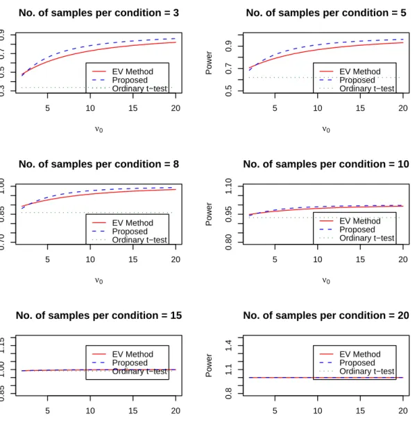
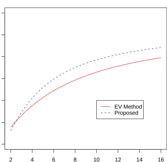
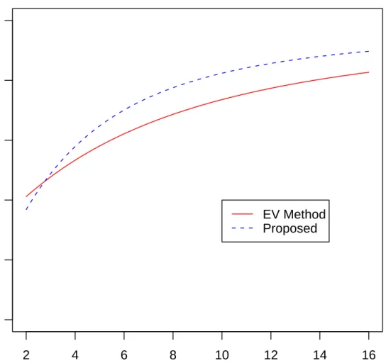
2.13 Power Comparisons . . . 41
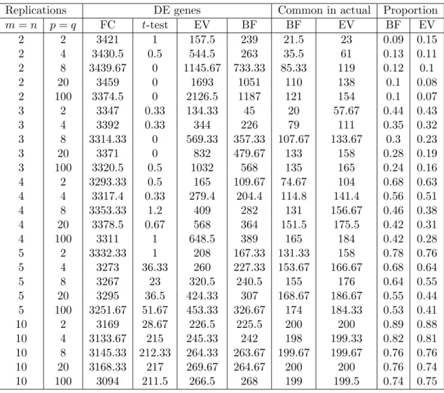
2.14 Comparison of DE Genes using the Window Method with Other Methods 46 2.15 Comparison of Proposed Method with other Methods . . . 50
2.16 Selection of Differentially Expressed Genes in the Golub Data . . . . 51
2.17 Transformation and Test of Normality Assumptions . . . 55
2.18 Conclusion . . . 58
3 Support Vector Machines and Other classification Methods 63 3.1 Summary . . . 63
3.2 Introduction . . . 63
3.3 Assumptions on Classification Methods . . . 64
3.4 Support Vector Machines (SVM) Methods . . . 64
3.5 Kernel Matrix and Kernel Tricks . . . 67
3.6 High Dimensional Feature Space for Large p Smalln . . . 67
3.7 Nearest Shrunken Centroids Method . . . 69
3.8 Weighted Voting Method . . . 72
3.9 Dudoit’s Multi-class Classification Method . . . 74
3.10 Gene Selection by Behrens-Fisher Statistic . . . 74
3.11 Choosing the number of genes required for classification . . . 77
3.12 Simulation and Results . . . 78
3.13 Datasets Pre-processing and Filtering . . . 79
3.14 MLL Leukemia Data . . . 79
3.15 Golub Leukemia Data . . . 82
3.17 Conclusion . . . 88
4 Selection of Differentially Expressed Genes in Correlated Statistics 89 4.1 Summary . . . 89
4.2 Introduction . . . 89
4.3 Effects of Correlations . . . 90
4.4 Application . . . 92
4.5 Computation of Effect of Correlations . . . 98
4.6 Conditional and Unconditionalp - values . . . 99
4.7 Dispersion Parameter . . . 100
4.8 Conclusion . . . 102
5 Performance of a Classifier taking into account of Correlated Genes 103 5.1 Performance of Classifiers . . . 103
5.2 McNemar’s Test and Confusion Matrix . . . 104
5.3 Filtering the Highly Correlated Genes . . . 105
5.4 Classification using SVM . . . 106
5.5 Application . . . 107
5.6 Confusion Matrices . . . 111
5.7 Binary Accuracy Measures . . . 113
5.8 Classification using the genes selected by the Correlated test Statistics 114 5.9 Conclusion . . . 114
6 Future Research 115
References 116
List of Tables
2.1 Multiple testing Procedure in Simultaneous Hypothesis Testing . . . . 20 2.2 Table of Power Comparison . . . 47 2.3 Comparison of BF test with other tests based on the proportion of
actually DE genes selected in Window Method. . . 48 2.4 Comparision of BF test with other tests based on the proportion of
actually DE genes selected in Similar Variance Method. . . 48 2.5 Comparision of BF test with other tests based on the proportion of
actually DE genes selected in Resampling Method. . . 49 2.6 Comparison of three methods ( I = Window Method, II = Similar
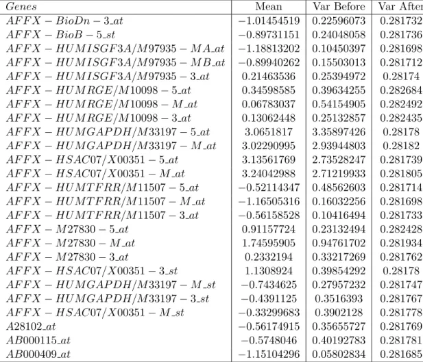
Variance Method, III = Resampling Method ) according to Proportion of truly DE genes selected, FDR and FNR. . . 51 2.7 Dependence of Variance on Expression level . . . 57 2.8 Comparision of Differentially expressed genes in Golub data controlling
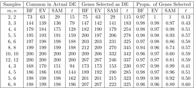
the FDR at the level α= 0.05 . . . 58 3.1 Accuracy Rate for the Simulated Test data . . . 79 3.2 Comparison of Classification Performance on MLL Leukemia Data. . 82 3.3 Comparison Classification of Golub Data using all the genes . . . 84 3.4 Comparison Classification of Golub Data using BF selected genes . . 84 3.5 Comparison of Classification Performance on Golub Data. . . 85 3.6 Comparison of Classification Performance on ALL-7 Data. . . 87 3.7 Confusion matrix for the MLL-3 training data by Dudoit method, and
Golub Test Data by NSC Method. . . 87 3.8 Confusion matrix for the ALL-7 test data by SCRDA method. . . 88
4.1 Goodness-of-Fit test of the test-statistics obtained by the BF method for the Golub Data . . . 93 4.2 Effect of Correlation on the standard deviations of the middle and tail
count of the transformed test statistics . . . 99 4.3 Effect of correlation on p-value on test statistics in Golub data . . . 100 5.1 Contingency table for misclassification . . . 105 5.2 Confusion Matrix for misclassification . . . 105 5.3 Classification of Golub Data taking into Correlation among the genes 108 5.4 Comparison of Classification Performance on Golub Data after taking
into correlation between the genes. Different percentage points were used to determine the optimal cut-point. . . 109 5.5 Comparison of Classification Performance on ALL-7 Data using the
genes Selected by the BF method and taking into correlation between the genes. The classes were compared using one versus another. . . . 110 5.6 Confusion Matrices of Test samples of Golub Data by Weighted Vote,
SVM and Dudoit methods . . . 111 5.7 Confusion Matrix of MLL data applying the Dudioit Classification
method after taking correlation . . . 111 5.8 Confusion Matrix of MLL data applying the Weighted Vote
Classifica-tion method after taking correlaClassifica-tion . . . 112 5.9 Confusion Matrix of MLL data applying the SVM Classification method
after taking correlation . . . 112 5.10 Contingency table for misclassification of Golub Test Data . . . 112 5.11 Contingency table for misclassification of MLL Test Data . . . 113 5.12 Confusion matrix derived accuracy measures, N =a+b+c+d . . . 113 5.13 Accuracy measures for the Wt. Vote, SVM, Logistic Discrimination
and Dudoit Multi-class Classifiers . . . 113 5.14 Classification of Golub Data taking into Correlated test statistics . . 114
List of Figures
2.1 Power comparison for different sample size and priors using Method 1 42
2.2 Power of the Proposed Method at m=n=3 . . . 43
2.3 Power of the Proposed Method at m=n=5 . . . 44
2.4 Graph of DE genes . . . 45
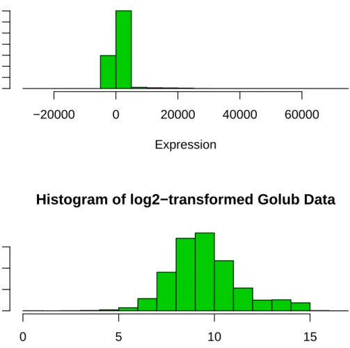
2.5 Histograms of Unprocessed Data Golub Data . . . 52
2.6 Histogram of log-2 transformed Golub Data . . . 53
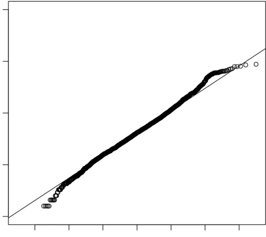
2.7 QQ-Plot of Golub Data . . . 54
2.8 Q-Q plot of some of the genes before Yeo-Johnson Transformation . . 60
2.9 Histogram of the T-values obtained by the BF Method . . . 61
2.10 Q-Q plot of some of the genes after Yeo-Johnson Transformation . . . 62
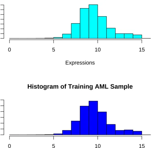
3.1 Histogram of Pre-processed AML Data . . . 80
3.2 Histogram of ALL,MLL and AML Training and Testing Data after Pre-processing . . . 81
3.3 Cross-Validation Error of Nearest Shrunken Centroid Method for MLL data . . . 83
3.4 Error Comparison for Golub data . . . 86
4.1 Histogram and the fitted Cauchy density curve for the BF test statistics 94 4.2 Histogram of transformed test-statistics . . . 95
Statistical Learning and Beherens-Fisher Distribution Methods for
Heteroscedastic Data in Microarray Analysis Nabin K. Manandhar Shrestha
ABSTRACT
The aim of the present study is to identify the differentially expressed genes be-tween two different conditions and apply it in predicting the class of new samples using the microarray data. Microarray data analysis poses many challenges to the statis-ticians because of its high dimensionality and small sample size, dubbed as ”small n largepproblem”. Microarray data has been extensively studied by many statisticians and geneticists. Generally, it is said to follow a normal distribution with equal vari-ances in two conditions, but it is not true in general. Since the number of replications is very small, the sample estimates of variances are not appropriate for the testing. Therefore, we have to consider the Bayesian approach to approximate the variances in two conditions. Because the number of genes to be tested is usually large and the test is to be repeated thousands of times, there is a multiplicity problem. To remove the defect arising from multiple comparison, we use the False Discovery Rate (FDR) correction. Applying the hypothesis test repeatedly gene by gene for several thousands of genes, there is a great chance of selecting false genes as differentially expressed, even though the significance level is set very small. For the test to be reliable, the probability of selecting true positive should be high. To control the false positive rate, we have applied the FDR correction, in which the p-values for each of the gene is compared with its corresponding threshold. A gene is, then, said to be differentially expressed if the p-value is less than the threshold.
We have developed a new method of selecting informative genes based on the Bayesian Version of Behrens-Fisher distribution which assumes the unequal variances in two conditions. Since the assumption of equal variances fail in most of the
sit-uation and the equal variance is a special case of unequal variance, we have tried to solve the problem of finding differentially expressed genes in the unequal variance cases. We have found that the developed method selects the actual expressed genes in the simulated data and compared this method with the recent methods such as Fox and Dimmic’st-test method, Tusher and Tibshirani’s SAM method among others.
The next step of this research is to check whether the genes selected by the pro-posed Behrens -Fisher method is useful for the classification of samples. Using the genes selected by the proposed method that combines the Behrens Fisher gene se-lection method with some other statistical learning methods, we have found better classification result. The reason behind it is the capability of selecting the genes based on the knowledge of prior and data. In the case of microarray data due to the small sample size and the large number of variables, the variances obtained by the sample is not reliable in the sense that it is not positive definite and not invertible. So, we have derived the Bayesian version of the Behrens Fisher distribution to remove that insufficiency. The efficiency of this established method has been demonstrated by ap-plying them in three real microarray data and calculating the misclassification error rates on the corresponding test sets. Moreover, we have compared our result with some of the other popular methods, such as Nearest Shrunken Centroid and Support Vector Machines method, found in the literature.
We have studied the classification performance of different classifiers before and after taking the correlation between the genes. The classification performance of the classifier has been significantly improved once the correlation was accounted. The classification performance of different classifiers have been measured by the misclas-sification rates and the confusion matrix.
The another problem in the multiple testing of large number of hypothesis is the correlation among the test statistics. we have taken the correlation between the test statistics into account. If there were no correlation, then it will not affect the shape
of the normalized histogram of the test statistics. As shown by Efron, the degree of the correlation among the test statistics either widens or shrinks the tail of the histogram of the test statistics. Thus the usual rejection region as obtained by the significance level is not sufficient. The rejection region should be redefined accordingly and depends on the degree of correlation. The effect of the correlation in selecting the appropriate rejection region have also been studied.
Chapter 1
Microarrays and Selection of Differentially Expressed Genes
1.1 Introduction
Deoxyribonucleic Acid (DNA) microarray technology was first mentioned in an article by Schena et. al. [38] published in the ’Genome Issue’ of Science in 1995 . After its publication, this technology attracted the attention of genome researchers. Nowa-days, it is one of the most advanced technologies to know the gene expression. In the course of understanding and deciphering the genomes of many organisms, there was a need for functional studies of thousands of genes across tissue samples. There was need for identification of expression patterns of genes under normal and pathological conditions. The access of genome sequencing was due to the development of high throughput DNA sequencing technology which created the system to approach biol-ogy. The most important throughput technology is the DNA microarrays technology which allows the researchers to make snapshots of genes in an organism in a single ex-periment. This technology allows the researchers to identify genes that are expressed in different cell types and conditions, to learn how their expression level changes in different developmental stages or disease states; and to identify the cellular process in which they participate. This technology produces a huge amount of information that can provide clues about how genes and gene product interacts and their interaction networks. But, transforming this data into knowledge is not a trivial task. Analysis using multiple techniques is needed to provide the comprehensive view of the under-lying biology.
In 1953, James Watson and Francis Crick [50] established the structure of DNA. The structure of DNA is a double helix, which is like a twisted ladder. Genes are made up of DNA and RNA (Ribonucleic Acid). Both DNA and RNA are polymers, that is, molecules that are constructed by sequentially binding the members of a small subunits called nucleotides into a linear strand or sequence. Each nucleotide consists of a base, attached to a sugar, which is attached to a phosphate group. The linear strand consists of alternate sugars and phosphates, with the bases protruding from the sugars. In DNA, the sugar is deoxyribose and the bases are Cytosine(C), Guanine (G), Thymine(T), Adenine(A). In RNA, the sugar is ribose and the bases are Cytosine(C), Guanine (G), Uracil(U) and Adenine(A). The genetic information of cellular organism is stored in long sequence of these four different bases that bond in a certain way - A bonds with T (or U), and C bonds with G via the hydrogen bonds. The sugar-phosphate backbone can, for the purpose of informatics, be considered as straight; though actually it has all sorts of twists, kinks and loops. The bases that protrude from the backbone are far more informative. The DNA is, thus, can be regarded as double stranded polymer. These DNA strands are complementary to each other meaning that every guanine (G) in one strand corresponds to a cytosine (C) in other complementary strand, and every adenine (A) in one strand corresponds to thymine (T) in the other complementary strand. The strings of nucleotides (bases) are the DNA molecules that compose the genome of an organism. These genome contain segments of DNA that encode genes. Genes are the functional and physical units of heredity that are passed from parent to offspring. Genes can be thought as a segment of DNA sequence that corresponds to a particular protein. Genome is the set of DNA molecules. DNA has two strands:
1. Sense strand 2. Anti-sense strand
Genes are transcribed into RNA called messenger RNA (mRNA) and are translated to form proteins. The RNA in the intermediate stage is called mRNA because it is used as a platform to form proteins from DNA and to pass the information to proteins
that is encoded by gene or DNA. These proteins are building blocks and functional units of a living cell. The process converting gene into proteins is called the gene expression. It occurs in two steps.
1. Transcription : The process of converting DNA into the mRNA 2. Translation : The process of converting mRNA into protein.
The information transfer from DNA to mRNA and mRNA to protein is called the
”Central Dogma of Biology.”
1.2 Gene Expression and Main Question of Interest
Each of the genes encoded in the DNA molecule either transforms into proteins through the transcription and translation or remains unchanged under that condi-tion. If the gene is transformed, then we say the gene is expressed in that condicondi-tion. DNA is a stable molecule and the same genomic DNA is present, with a few exception, in all cells of living organism. Despite this all the cells are not the same, like-hair, muscle, skin cell etc. Why? The difference between the cells is due to the different subset of genes that are expressed in each of the different cell types. Different subset of genes are expressed in response to stimuli so that the pattern of gene expression level reflects both- type of cell and its condition. The amount of each mRNA detected in the cell can provide information on the corresponding protein and the relationship between abundance of mRNA and formation of protein.
1.3 What is microarray and how does it work ?
A microarray is typically a glass/ polymer slide onto which DNA molecules are at-tached at fixed locations, called spots or features. There may be tens of thousands of spots on an array- each spot containing tens of millions of identical DNA molecules. For gene expression, each of these DNA molecules should identify (transcribe) to a single mRNA molecule in a genome. The features are either printed on the microar-rays by a robot or a jet; or synthesized in situ by photolithography, or by ink-jet
printing. The most popular microarray application is to compare the expression lev-els of genes in two different samples; e.g. the same cells under two different conditions. This is done by labeling the mRNA obtained by the reverse transcription method, extracted from each sample of two different ways by two colors-green from the normal and red from the experimental condition. The hybridized microarrays is excited by a laser and scanned at wavelengths suitable for the detection of red and green dye intensities.The amount of florescence emitted upon laser excitation corresponds to the amount of nucleic acid bound to each spot. If the nucleic acid from sample condition 1 is abundance, the spot appears green, while if from condition 2 is abundance, it ap-pears red; if both are equal, it apap-pears yellow; and if neither present, apap-pears black. Thus from the florescence intensities and colors of each spot, the relative expression levels of the genes in both samples are estimated. Hence, thousands of data points and information of expression levels of a particular transcript can be obtained from a single experiment. Two types of microarrays are currently available.
1. cDNA microarray
2. Oligonucleotide microarray
1.4 Oligonucleotide microarray
These are the list of terms that are used in this type of microarrays. Probe: oligo-nucleotides of 25 base pair length used to probe RNA targets. Perfect Match:
probes intended to match perfectly the target sequence. PM: intensity value read from the perfect matches. Mismatch: the probes having one base mismatch with the target sequence intended to account for non-specific binding. MM: intensity value read from the mis-matches. Probe Pair: a unit composed of a perfect match and its mismatch.
Oligonucleotide arrays are used to measure the abundance of mRNA transcripts for many genes simultaneously. 11 to 20 perfect match (PM) and mismatch (MM) probe pairs are used to measure the expression level of each gene. Here is an example
of probe and PM and MM: Probe Pair: This consists of the 4 kinds of bases: A,C, G, T. Generally, 25 of these base sequence is selected from the gene of interest.
5”...A GGG T G CCCCTTTG AAA...3” (sense strand) 3”...T CCC A C GGGGAAAC TTT...5” (antisense strand)
to
5”...A GGG U G CCCCUUUG AAA...3” 3”...U CCC A C GGGGAAAC UUU...5”
translation into mRNA
The only difference between DNA and RNA is that the base thymine (T) is replaced by the base uracil (U).
Examples of PM and MM probes:
PM probe: ATGATCTCGAATAGCGTGCGCGAAT MM probe: ATGATCTCGAATTGCGTGCGCGAAT
This is an example of probe pair. 11-20 such probe pairs of 25-bases is chosen in each spot of microarray to get the expression of a gene. The polymer such formed is also called a probe for a gene. The two probes are called complementary to each other. The only difference between PM probe and MM probe is that the middle base (A in the above example) is flipped to its complementary base T. Then simple or weighted/robust average of the difference PM-MM of all probe sets is taken. This is called the average difference which measures the abundance of mRNA in the oligonu-cleotide affymetrix data. The human genome has about 2.8×10⁹ base pairs and it encodes at least 40,000 genes.
1.5 cDNA Microarray
The mRNA from two tissues are extracted, separately reverse transcribed, and la-beled with different colors- green (Cy3), red (Cy5). The mixture lala-beled cDNA are hybridized onto the different spots of glass slides (called microarray). These spots already contains the abundance identical probe sequence of complementary DNAs. Thus the colored cDNAs compete to bind (hybridize) to their complementary cDNA in each spot. After hybridization, the microarray slide is washed and they are scanned at different wavelengths by a laser or by a charged-coupled device (CCD) camera to obtain numerical intensity of each dye. Since the values thus obtained are so large, the statistical analysis are done transforming into log(cy5/cy3). Generally base 2 is taken because, it equivalently transforms up-regulated and down-regulated genes. The intensities ranges from 0 to 216.
The advantage of cDNA microarray is that they can be prepared directly from the isolated clones. Once the set of corresponding PCR products has been gener-ated, microarrays can be created in multiple versions containing the entire set of cDNA sequences, resulting in the large-scale arrays for identification of differentially expressed genes of nterest.It is less expensive to prepare. The cross-hybridization be-tween homologous sequence is problematic for cDNA microarrays. The advantage of oligonucleotide microarrays is that they can be synthesized either in plates or directly on solid surfaces; making it easier to prepare. They are expensive and the probes in such array can be designed to represent unique gene gene sequences so that the cross hybridization between related gene sequences is minimized to a degree depen-dent upon the completeness of available sequence information.
Microarrays are applied to different situations. It helps to find the genes that are differentially expressed in different conditions. So, it has enormous importance in the field of Bio-medicine and Genomic. For example, as mentioned in the paper of Efron et al. [12], some cancer patients have severe life- threatening reactions to radiation treatment. So, it is important to recognize the basis of this sensitivity, so that such
patients can be identified before treatment is given. The treatment is life threatening, so if given to such patients who are sensitive to radiation it can threaten life and hence decision should be taken before use.
1.6 Measuring the Expression Levels of a Gene
The starting point of any statistical analysis begins from the estimation of expression level of each gene in the microarray. To measure the real gene expression, we have to measure the abundance of proteins. However, DNA microarray experiments measure the abundance of mRNA, but not the protein abundance. According to the simple traditional view of gene expression, there is a direct one-to-one mapping from DNA to mRNA to protein. To put in another way, a specific gene (i.e. genomic DNA sequence) always produce one and the same amino acid sequence of corresponding protein, which then fold to assume its native state. Given this simplified scheme, measuring the mRNA abundance would provide us with highly accurate information on protein abundance, as protein and mRNA abundance are proportional to direct mapping. There are thousands of spots (features) in a microarray slide. Each spot is associated with just one gene. For each gene/spot/feature, the amount of mRNA present is measured by the principle:
Amount of florescence emitted ∝ αm, where, m is the amount of mRNA present
in the spot.
To measure the expression level, the hybridized microarray is excited by the laser and scanned at the wavelengths suitable for the detection of both red and green inten-sities. From the florescence intensities and color of each spot/gene, we measure the expression level of the gene in the spot. Suppose that for gene g,
Rg = expression level ( florescent intensity) of gene g in query sample
Gg = expression level(florescent intensity) of gene g in reference sample, and
Tg =
Rg
is the ratio of intensities between query and reference sample. • If the spot appears red, then T >1.
• If the spot looks yellow, then T = 1. • If the spot appears green , then T <1. • If the spot appears black, T is undefined.
Similarly, for the two sample with replication, we measure the expression levels of green and red intensities of the same gene at more than one spot and we get the values of expression for two different condition.
The quality filtering is implemented to produce good quality of intensity measure-ment. For this, one uses the multiple spot replication slides. Multiple spotting of target DNA on a slide provides a means to assess the quality of data for a gene on that slide. Suppose each gene is spotted p times on the slide. For each spot, a ratio of Cy3 and Cy5 intensity is calculated as m = Cy3/Cy5. Let CV = σ/m¯ be the coefficient of variation of the set of ratios m1, m2, ..., mp on the multiple spots. The
quality of the data on the expression level of each gene is inversely related to its CV. For each gene, a window subset containing 50 genes whose mean intensities are closest to the gene of interest is constructed. The CV of each gene is calculated and ordered in the increasing order. If the CV of the gene of interest falls within the top 10% of the CV’s then we discard this gene saying it has poor quality.
1.7 Statistical Methods for Differentially Expressed Genes
An exciting development in genomic is the use of microarray technology to simulta-neously monitor the expression levels of thousands of genes. A common task is to compare the expression levels of genes in samples drawn from two different condi-tions. Specially, it is of interest to detect genes with differential expression under two different conditions. In early days, the simple method of fold-change was used and now it is known to be unreliable (Chen et al. [7]) because statistical variability
was not taken into account. Since then many more sophisticated statistical meth-ods have been proposed ( e.g. Chen et al.[7]; Efron et al. [12]; Newton et al.[29]; Tusher et al.[48]; Pan et al. [30]). It has also been noted that the data based on a single array may not be reliable and may contain high noises. As the technology advances, microarray experiments are becoming less expensive , which makes the use of multiple arrays (or multiple spots on each array) feasible. Hence it is possible to use the test that requires replicated measurements of expression levels of each gene under two different conditions. A straight forward method is to use the traditional two sample t-test. Thomas et al. [46] proposed a regression modeling approach. Pan
et al. ([30]) suggested the a mixture model approach, which follows the basic idea of
Efronet al. [12]and Tusheret al. [48]. On the other hand there are different methods using Bayesian and empirical Bayes method. Other methods are the linear models and empirical Bayes method of Smyth (2003 )and ANOVA approach of Kerret al.[22]. The other efficient methods are given by Florence et al. 2007 based on the Johnson’s distribution.
1.8 Methods for cDNA Data
A number of methods have been suggested for the identification of differentially ex-pressed genes in single-slide two-color microarray experiments. In such experiments, the data for each gene consist of two fluorescence intensity measurements. Let R and G be the expression level of the gene in the red (Cy5) and green (Cy3) la-beled mRNA samples respectively. Generally, the data consists of the value of the logarithmic base two of R/G. The advantage of this transformation is that it pro-duces a continuous spectrum of values for differentially expressed genes while treat-ing up-and down-regulated genes equivalently. For example, if the expression ratio R/G = 4,2,1,1/2,1/4, the logarithmic base 2 has values 2,1,0,−1,−2. So, if the data is transformed by logarithmic base 2, then an up-regulated gene by 4 has value 2, and down-regulated gene by 4 (ratio = 1/4) has value −2.
Early analysis of microarray data (Schena et al., [38]) relied on the fold change cut-offs to identify differentially expressed genes. Typically a fold change equal to
2 or 3 is taken as the cut-off. If a gene has logarithmic base 2 ratio greater than 2 then the gene is said to have differentially expressed. Schena et al.[38] used a spiked control in mRNA samples to normalize the signals for the two fluorescent dyes and declared a gene as differentially expressed if the difference of the expression levels is more than 5 in two mRNA samples.
Let mg = log2RGgg be the log expression of gene g. If m0g = log2R 0
g
G0
g be the log
ratio of N ”housekeeping genes”, that is the genes believed not to be differentially expressed between two conditions of interest. Let m0 be the mean and s0 be the
standard deviation of these house keeping genes. De Risi et al.( 1996)[8] declared the genes as DE if
|mg −m
0
s0 |>3 (1.8.1)
A slightly more sophisticated approach involves calculating the mean and the standard deviation of the distribution of the ratio mg and defining the global fold
change difference and confidence. The ratio-intensity plot reveals that the data has more variability at lower intensities and less variability at higher intensities. So, using a sliding window at each gene we can access the local structure of the data to determine its differentiability. Let ¯xg and sg be the mean and standard deviation of
log-2 ratio of gene g calculated by taking all the genes within the window, then
zg =
¯
xg
sg
(1.8.2) is normally distributed with mean zero and standard deviation 1. Declare the genes as differentially expressed if |zg| > 1.96. At higher intensities, sg will be bigger and
allows changes to be identified where the data is more variable.
Kerr et al. [22] introduced the use of ANOVA models that accounted for
ar-ray, dye, and treatment effects for cDNA arrays. In this fashion, normalization was accomplished intrinsically without preliminary data manipulation. The model they proposed can be written as
where, µ is the mean expression, Ai is the effect of the ith array, Tj is the effect of
the jth treatment, Dk is the effect of the kth dye, Gg is the effect of the gth gene,
and AGig and T Gjg are the interaction effects. Of interest for testing the differential
expression are the interaction effects, T Gjg, for which appropriate contrast can be
estimated for each gene. in this model all effects were considered as fixed effects and other terms could be incorporated in the model.
1.9 Methods for Oligonucleotide Data
To detect the DE genes between two different conditions, the two sample t-test and its variants have been frequently used. Specifically, if we have samples from two conditions, the t-statistic is given by
t= x¯2−x¯1 sq 1 n1 + 1 n2 (1.9.4)
where, ¯x are the means ands is the pooled sample standard deviation.
It is hard to verify the underlying assumption of normality because of small sample sizes perfectly, but with the common technologies this assumption is reasonable for the logarithm of the expression levels [1], [13], [11]. Baldi and Long [1] proposed a Bayesian version t-statistic using the priors. More specifically, if thexc
1, xc2, ..., xcnc and
yt
1, y2t, ..., yntt be the log transformed expression levels in the control and treatment
conditions respectively, they have assumed the data has been transformed into the form such that normality assumption holds. So x ∼ N(µ, σ2). The priors for means and variance has been chosen as
p(µ|σ2) = N(x;µ0,σ
2 0
λ0
) p(σ2) =IG(x;ν0, σ02) (1.9.5) where, IG is the scaled inverse gamma pdf with degree of freedom ν0 >0 and scale
σ0 >0 IG(x;ν0, σ02) = (ν0/2)ν0/2 Γ(ν0/2) σν0 0 x−(ν0/2+1)exp(− ν0σ20 2x )
The prior is obtained as
p(µ, σ2) =p(µ|σ2)p(σ2).
With this prior, the posterior was of the same form as prior, hence it was theconjugate
prior. Taking µ0 = ¯x and using the mean of the posterior distribution, the maximum a posteriori (MAP) estimate for mean µ and variance σ2 was shown to be
ˆ µ= ¯x σˆ2 = ν0σ 2 0 + (n−1)s2 ν0+n−2 (1.9.6) Other researchers used the log-normal and gamma-gamma model to detect the DE genes ( Newton et al., [29]). Since the small variance gives rise to large t-statistic, empirical Bayes (EB) method of analyzing microarray data was used by Efron et al.[12] without assuming any distributional assumption of the data. They slightly tuned the t-statistic by adding a suitable constant, a0, which is generally taken as 90th percentile of standard deviation, on the Z-score obtained like in t-test,
Z = D¯i
a0+Si
where,Si is the standard deviation of the ith gene. Ifp1 (p0) are the prior probability that the gene is expressed (not expressed), p1(z) (p0(z) are the posterior probabilities of a gene is expressed (not expressed), f1(z) (f0(z)) be the density of the expressed genes, then the mixture density for a gene is given by
f(z) =p0f0(z) +p1f1(z). (1.9.7) The densities f0(z) andf1(z) were estimated from the data without assuming any dis-tribution, so it was called the Empirical Bayes approach. The posterior probabilities can be written as p1(z) = 1−p0f0(z) f1(z) , p0(z) = p0f0(z) f1(z) (1.9.8)
The ratio f0(Z)
f1(z) was obtained by fitting the logistic regression model
logit(p1(z)) = β0+β1z (1.9.9)
and the priors p0 and p1 were estimated by
p1 ≥1−min z f(z) f0(z) , p0 ≤min z f(z) f0(z) (1.9.10) The estimate of the sample variance is not reliable for small sample data, specially in the case of microarray data, Tusher et al. (2001) [48] proposed the statistical analysis of microarray (SAM) method to stabilize the effect of large variances arising from low expressed genes. In this method, the SAM statistic is the same as in (1.9.4) but a small fudge factors0 is added in the denominator. The value of the fudge factor is chosen so that the coefficient of variation of thet-statistics is constant as a function of standard deviations. Generally, 90th percentile of si is used as the fudge factor.
After estimating the fudge factor, the t-scores is ranked in the decreasing order of t-statistics, i.e. t(1) ≥t(2)≥ ...≥ t(p), where,p is the number of genes. To select the threshold ∆ to determine the genes witht-scores greater and/or smaller than the threshold are differentially expressed, SAM uses the permutation of columns(arrays). The first n1 of the permuted columns are taken to be as from condition 1 and the remaining columns are taken to be as from condition 2. We permute the arrays, say-B times. In each permutation b = 1,2, ....B, the t -score thus obtained is ranked, say
tb(1) ≥ tb(2) ≥ ... ≥ tb(p). The expected order statistics of gene g is calculated
by tE(g) = B1 PB
b=1tb(g). This means that look the gth descending ordered row
g = 1,2, .., p of each column and take the average. This gives the expected order of
gth ordered gene t(g) in the original ordering. The false discovery rate is calculated by ˆ F DR= 1 B PB b=1Nb N
where, Nb is the number of genes in the bth permutation that has expected score
respec-tively, and N is the number of genes that has originalt-score smaller or greater than t(g0) and t(g∗) respectively.
1.10 Assessing the Reliability of Tests
The p-value was invented for testing the single hypothesis. But, in microarray data, there are thousands of genes, so, we need to test thousands of hypothesis simulta-neously. In the case of repeated testing of hypotheses, the p-value is conceptually associated with the specificity of the test, i.e. it is used to control the false pos-itive rate of a test. Declaring a test to be significant when p-value < 0.05 means that we are setting specificity 0.95. False discovery rate (FDR) of a test is defined as the expected proportion of false positives among the declared positives/significant results. If we declare 100 genes are significant and FDR is 0.1, then this means that we expect maximum of 10 out of 100 genes are false positives. No such interpretation is available from thep-value. The false negative rate (FNR) is defined as the expected proportion of true negatives out of actual positives. When controlling the FDR, one need to control the sensitivity or FNR. Setting FDR too low means that FNR is high. This means that the chance of including truly differentially expressed genes as not differentially expressed is high. So, FDR must be accompanied by sensitivity. Factors determining FDR:
1. Proportion of truly differentially expressed (DE) genes 2. Distribution of true differences
3. Measurement variability 4. Sample size.
What is the relation between sample size and FDR ? Any statistical testing pro-cedure applied on the gene by gene basis is characterized as follows:
• Sort the statistic in order
• Determine a cut-off point beyond which all the genes are significant
Pawitanet. al. [32] has shown that, if we declare top (1−p0)×100% as DE genes, then FDR=FNR. For a microarray test, generally one expects F DR = F NR. Now to answer the question : To answer how the sample size affects the different rates (i.e. FDR, FNR, sensitivity), they proved that, as the sample size increases then the FDR decreases and the sensitivity (power) increases. FDR and sensitivity totals 1, so FNR decreases as the sample size increases. Given a true proportion of not-DE genes, the paper discusses the different rates as a function of the critical values. It then discusses the effect of sample size on the different rates. Again it discusses the different rates as the function of percentage of significant genes ( obtained according to the top ranking genes). When one declares a small proportion of top genes as differentially expressed, it can lead to low sensitivity / large FNR. Sensitivity of a test increases with the number of samples per group. One can get high sensitivity declaring more proportion of top genes, but the small FNR has to pay a price for high FDR. So, declaring few top genes as DE is not only the solution of the problem of gene selection. What should one expect if one declares genes in the basis of critical values, as in t-statistic? When one declares genes on the basis of two sided test and critical values like t-test, then again the problem is due to the high FDR. In this case one must have big enough sample size to get high sensitivity and low FDR. It does not work for the small sample sizes like 5 samples per group but works well for 30 samples per group. Furthermore, it depends on the true proportion p0 of non-DE genes. If p0 is 0.99, this method also does not produce the satisfactory result even for sample size is large. But, on the other hand, ifp0 is small, say 0.9, then it works well. If one chooses the method of fold change, one must choose the fold change of at least 3 times standard deviation to get better result.
1.11 Conclusion
In this chapter we have reviewed the literature about the microarray data analysis. The basic concepts of microarray data, how the expression of genes are measured and how these data are useful for identifying the differentially expressed genes. We have revisited some of the tools to analyze these data, why the microarray data is difficult to analyze and simple statistical tool is not effective for analyzing such a data. Furthermore, we have introduced the factors that should be taken care into account while identifying the differentially expressed genes.
Chapter 2
Behrens-Fisher distribution for selecting Differentially expressed Genes
2.1 Summary
In this chapter, we will derive an expression for the test statistics in the case of het-erogenous variances in the two samples using the Behrens Fisher distribution. Since the sample variances obtained from the microarray data are not a better estimates of the population variances, we use the priors for the estimation of variances. Then we compare the powers in the case of equal and unequal variances and study the effects of the variance in calculating the test statistics for the thousands of genes. We have compared the proposed method with other existing methods such as the equal variance method of Fox and Dimmic [13], the data dependent method of SAM [48], simple two sample t-test [4] and LIMMA [41] for the small sample size settings.
2.2 Introduction
The two sample t-test is one of the most popular methods for testing the difference between two samples [1], [13],[48]. There are different versions and variants of these tests: non-parametric and Bayesian version. In such tests, one is primarily interested on the identification of differentially expressed genes under two different conditions, so that those particular genes of interest are further studied. Most of the existing methods used in the literature for identification of differentially expressed genes are two-samplet- tests [35], [17], [1], [48] and its variants, SAM [48] and regularizedt-test
[1]. In thet-test, the variances of each of the genes in account together with the means. In this test, a gene is said to be expressed if |t|exceeds a certain threshold depending on the confidence level selected. Since the distance between the sample means are standardized by the variances, this approach is better than the fold-change method. The gene expression data shows that there is an inherent limitation behind using the simple two-sample t-test. The variances of the genes depends on the expression level [35], [1], [48]. To identify the genes that are actually expressed, one should consider this fact. This fact was considered in the earlier works [17], [48].
There are two inherent problems in microarray experiments: First, the number of replications is very small, and second the number of genes to be tested is usually large and the test is to be repeated thousands of times. Since the small population size is very common in microarray studies, the sample estimates of variances are not appropriate for the testing. The variance of genes depends on the expression level [48], [35], [1]. Therefore, we have to consider the Bayesian approach to approximate the variances in two conditions. To remove the second defect arising from multiple comparison, we use the False Discovery Rate (FDR) correction [54]. Applying the hy-pothesis test repeatedly gene by gene for several thousands of genes, there is a great chance of selecting false genes as differentially expressed, even though the significance level is set very small. For the test to be reliable, the probability of selecting true positive should be high. To control the false positive rate, we have applied the FDR correction, in which the p -values for each of the gene is compared with its corre-sponding threshold. A gene is, then, said to be differentially expressed if the p-value is less than the threshold.
The Behrens - Fisher problem arises when one seeks to make inferences about the means of two normal populations without assuming the variances are equal. But, in many practical situations the populations do not have same variances. Although the Satterthwaites t-test deals with the unequal variances case, the degrees of freedom is small and hence it does not produce better estimate of the variances [1]. Here, we
briefly review the two sample t-test and introduce the proposed Behrens Fisher (BF) distribution.
Let x= (x1, x2, ..., xm) and y = (y1, y2, ...., yn) be two independent samples from
two normal populations with means µx and µy and equal variances σx2 = σy2 = σ2
respectively. If ¯x and ¯y are means; s2
y and s2y are variances of x and y respectively;
and s2 = (m−1)s2x+(n−1)s2y
m+n−2 is the pooled sample variance, the two sample test statistic is given by
t= pδ−(¯y−x¯)
(1/m+ 1/n)s2
is distributed as student’s t-statistic with (m+n−2) degrees of freedom.
Now, let the samplesxandyare from normal distributions with unequal variances
σ2
x andσy2 respectively. In this case neither a pivotal statistic nor an exact confidence
interval procedure exist [23]. We can take a statistic
t∗ = qδ−(¯y−x¯)
s2
x/m+s2y/n
∼t[min(ν1,ν2)]
where, ν1 = m−1, ν2 = n−1. If the sample sizes m and n are large, then the both t and t∗ statistics give almost the same result. In the microarray experiments
the sample sizes are relatively small, thus motivating us to look for an alternative.
2.3 Multiple Testing
To select the differentially expressed genes from thousands of genes, there are thou-sands of hypotheses each belonging to each gene. So the hypotheses must be tested simultaneously. For this, the hypothesis tests should be run thousands of times re-peatedly. A problem with doing so many tests is that the number of false positives may be increased. This phenomenon is called multiple testing. The simultaneous hypotheses is:
Number of Genes Declared non-DE Declared DE Total
True non DE U V m0
True DE T S p−m0
p−R R p
Table 2.1: Multiple testing Procedure in Simultaneous Hypothesis Testing
H0 :
Gene 1 is not differentially expressed Gene 2 is not differentially expressed
... ... ...
Gene p is not differentially expressed.
(2.3.1)
H1: At least one Gene is differentially expressed.
While testing the simultaneous hypotheses, one gets the number of hypotheses as in the table. Similar to testing a single hypothesis, the idea here is to control the number of false positives, V. This number is a random variable whose value differs from one test to another test. Let α be the type-I error that one makes when testing for a gene i. Then, α = Probability of rejecting H0 in fact H0 is true. In terms of above hypothesis, α= Probability of selecting a false gene as differentially expressed. Such a gene is called a false positive. So, expected number of selecting false positives from a set of p genes isαp. In other words, since p is very big integer, the number of false positives in the experiment is very big, even though we choose α very small.
This means that, probability ofnot selecting a false gene as differentially expressed = 1−α. In other words, probability of making the right decision for a gene = 1−α. Hence, the probability of making correct decision for all p genes = (probability of making correct decision for gene 1).(probability of making correct decision for gene 2)...(probability of making correct decision for gene p) is (1−α)p. From this we
see that, as p increases, the probability of making correct decision decreases. So, the probability of at least one false positive somewhere is:
This Type I Error is also called the family-wise error rate (FWER). There are few approaches to minimize the family-wise error rates. If the FP Rate is the error mea-sure used, then a simple p-value threshold of α guarantees that the expected number of false positives, V, when testing allp hypothesis/genes is E(V)≤αp.
1. Sidak and Bonferroni Correction
This multiple correction method is one of the earliest method introduced by Bon-ferroni [54]. Let p be the number of tests performed for each gene. Let us consider a problem of achieving a global significance level α. Now the question is what value of gene-wise significance level αg should be specified to achieve this goal ? From (2.3.2),
this means that,
rectionα= 1−(1−αg)p
or, αg = 1−(1−α)
1
p (2.3.3)
The above equation(2.3.3) is called the Sidak Correction for multiple testing. This means that if we want to achieve the global significance level αg, we have to set the
significance level for each gene as 1−(1−αg)
1
p. Expanding the (2.3.3) by Binomial
theorem and taking the first two terms we get the Bonferroni Correction :
α= 1−(1−αg)p = 1−(1−pαg +...) =pαg (2.3.4)
or,
αg =
α
p (2.3.5)
This means that instead, we have to set the significance level as α divided by the number of genes (tests to be performed). In other words, if the error measure is FWER, then the probability that at least one false positive gene will be selected by the rule when we set αg = αp does not exceed α. From the above, the significance
the following method was proposed.
2. Holm’s Step-wise Correction:
While the Sidak and Bonferroni approaches [54] are effective to avoid too many false positives, but the worst that can happen is : we get none of the genes signifi-cantly expressed because we take the same significance level for all tests (genes) and the significance level αg
p is too small for largep. So, this method is tooconservative in
the sense that it selects the only strong truly DE genes. Because of large number of hypotheses, p, there is many false positive by chance, it is more appropriate to choose the significance level for a gene according to its p-value. This method adjusts more to the genes that have smaller p-values than on larger p-values.
Algorithm:
1. Choose the global significance level α.
2. Order the genes according to their p-values in ascending order.
3. Compare the p-value (pi) of the i-th gene in the ordered list with the threshold
τi = p−αi+1.
4. Report the gene i in the order as significantly expressed ifpi < τi.
Here, what we see is that the threshold for the genes is chosen according to their p-values. If the p-value for a gene is smaller then the order i is smaller. Hence τi is
also smaller. This makes more sense than the uniform significance level.
2.4 Measures of Erroneous Rejection of Null Hypotheses
There are two measures of false decision in the multiple testing context as described in [54]:
2. False Discovery Rate (FDR)
The FWER is defined as the probability of at least one false positive:
F W ER=P rob(V ≥1).
The false discovery rate is defined is given by
F DR=E · V R|R >0 ¸ ×Prob[R >0].
where, V = number of false positives; R = V + S, number of positive findings. Generally, F W ER ≥ F DR. Equality holds if all null hypotheses are true. But, in practice, some null hypotheses are actually false, hence FDR control is less strict than the FWER control, hence it has more power [52]. So, instead of controlling the FWER, Benjamini and Hochberg [3] proposed a method to control the FDR. The FDR is estimated by the permutation scheme. Depending on the chosen cut-off value(s) α for the test statistic Tg one can estimate the FDR as follows:
• Estimate the number of non-differentially expressed genes,m0. This can be done in the following way:
– Calculate the p-values for each of the genes. A gene g with pg > 0.5 is
usually not differentially expressed.
– Since thep-values of non-differentially expressed genes should be distributed uniformly on [0,1], the estimate of m0, ˆm0 = 2∗#{g :pg >0.5}.
• Compute the number of significant genes under permutations of the sample labels. The average of these numbers, multiplied with ˆm0/N gives an estimate of the expected number of false positives, \E(V).
In other words, ifαbe the significant level of the test,m0be the truly non-differentially expressed genes and R be the declared differentially expressed genes, then
F DR = α×m0
R .
If all the null hypotheses were true, then the FDR is equal to the familywise error rate. However, this rarely happens in reality. In general, the more the number of hypotheses that are truly false, the smaller is the FDR. Therefore, the control of FDR tends to be more relaxed than control of FWER at the same level of significance. To determine the differentially expressed genes using the FDR procedure, one uses the following steps:
• Choose the global significance level α
• Order the genes according to their p-values in the increasing order.
• Compare the p-values (pi) of the i-th gene in the ordered list with threshold
τi = piα.
• Report those genes i as differentially expressed which satisfies pi < τ i.
Storey and Tibshirani [43] noted that an adjustment is only necessary when there are positive findings, i.e.there are cases when the null hypotheses are rejected. They proposed the modified version of the FDR, called the positive false discovery rate
(pFDR):
pF DR=E[V
R|R >0]
Since the number of false positives are unknown, we have to estimate V in order to estimate pFDR. Suppose we have a dataset of N genes in two conditions replicated n1 andn2 times. Then change the class labels by permuting each geneB times. Suppose that the average number R∗ of genes have the p-values smaller than threshold α (where α is the genewise significant level) over theB permutated data sets.Then the estimate of the pFDR is:
pF DR= R∗ R
Since the calculation of FDR is based on the gene scores from permutations of the data, the correlation in the genes are accounted for. Use of the permutation distribution avoids the parametric assumptions about the distribution of individual genes. Hence, the FDR criteria of selecting genes is usually better than the FWER criteria of selecting genes, because FDR takes account of correlation among the genes and it is more powerful.
2.5 Two-Sample Permutation Test
In the two sample t-test, one requires the following three assumptions: • the samples are randomly selected from two populations
• the populations have normal distributions; and • the variances of two populations are same.
If anyone of the above assumption fails, then it is likely thatt- test can not give more accurate result. Furthermore, the sample size in the microarray experiment is usually too small. So, the random assignment of the observed intensities of each geneiin two different conditions provides the basis for drawing statistical inference about the effect of the treatment over the normal condition. The argument goes as follows: Consider a single gene i. If there is no difference between normal and treatment conditions (i.e., it expresses similarly in both conditions), then assigning randomly all the values obtained between two conditions would have an equal chance of being observed in the study.
For example, let there are 3 values under normal condition and 2 values under treatment condition of gene i. Then there are C(5,2) = 10 combinations of different genes altogether, in each conditions. These are the types of datasets one would expect to observe if the gene i under two conditions are equally expressed. Since we have permuted the label of each gene in two conditions, we expect that the mean of two
samples are equal. This means we can use the difference of means as the test statistic. Let Dobs be the difference between two observed sample means. Then we have 10
different means of differences D of permuted samples. Then for the two-tailed test, the p-value for the gene iis given by:
pi = number of |D|
0s≥ |D
obs|
number of permutations
With this p-value, reject the null hypothesis at the level of 5% significance level,
i.e. if p-value <0.05.
2.6 Significance Analysis of Microarrays (SAM)
Although the permutation based approach proposed by Westfall and Young (1991) [51] defines weak control of the error rate and considers the correlation among genes, it is still too stringent to their data. In their experiment, they identified either zero or 300 significant genes depending on how the p-value is corrected. To address the above challenges, Tusher et al.[48] proposed the Significance Analysis of Microarray (SAM) . Basically, SAM assigns a score for each gene according to the change in gene expression. Genes with greater than the threshold is considered to be potentially significant. To control false positives, SAM uses the permutation of measurements to estimate the pFDR [48]. The score threshold for genes is then adjusted iteratively according to the pFDR until a set of significant genes have been identified. To each gene i, SAM assigns a score
d(i) = x¯1(i)−x¯2(i)
s(i) +s0
, (2.6.6)
where ¯x1(i) and ¯x2(i) are the average level of expressions for gene i in the classes 1 and 2 respectively. If there are n1 and n2 replications of gene iin two classes,
s(i) =
s
(n1−1)s21+ (n2−1)s22
n1+n2−2
denom-inator.The reason behind it is, the variance s(i) tends to be smaller at the lower expression levels. This makes the score d(i) dependent ins(i). To compare the values of d(i) across all genes, the distribution of d(i) should be independent of expression levels and hence independent ofs(i). To address this problem, SAM seeks to find the fudge factors0 such that the dependency ofd(i) withs(i) is as small as possible. Such an s0 is obtained by certain percentile of si values depending on the data. The FDR
in the SAM procedure is obtained by the permutation method, which is different than the Benjamini and Hochberg procedure. It is given by
pF DR= 1 B PB b=1Cb C
where B is the number of permutations of samples, Cb is the number of potentially
significant genes in the b-th permutated data set, and C is the # of potentially significant genes in the original data set.
2.7 Sampling Distribution for Non-homogeneous Variance 2.8 Bayesian Approach
In the following, we are going to derive the marginal posterior distribution of the difference of two population means from two samples with different variances. We have taken the priors as in [1], and we have compared the result with the existing method [13]. Since there are few samples in the microarray data, all the information required to estimate the parameters are not sufficient. So, as in Baldi and Long [1] and [13], the Bayesian approach has been proposed to estimate the distribution and estimate the parameters.
For the samples x = (xi) iid∼ N(µ, σ2) and y = (yj) iid∼ N(µ+ ∆µ, τ2),where,
The density forx= (x1, x2, ., ..., xm) can be written as , f(x) = 1 σm(2π)m2 exp h−1 2σ2{(m−1)s 2 x+m(¯x−µ)2} i (2.8.7) Similarly, the density of y is,
f(y) = 1 τn(2π)n2exp h−1 2τ2{(n−1)s 2 y+n(¯y−µ−∆µ)2} i (2.8.8) The frequentist approach requires a large number of observations before making the probabilistic judgements about the outcomes. In the microarray data, the sam-ple size is small thus it underestimates the population variance and gives unreliable estimate of the population variance. Classical statistics are directed towards the use of sample information in making inferences. But in Bayesian analysis, one combines the information obtained from sample and other relevant aspects of the problem in order to make the best decision. So, we use the bayesian analysis for estimating the variances. For microarray data the conjugate prior seems to be more suitable and flexible because of its convenient form. Assuming the independency of the location parameter µ and scale parameter σ2 as in [13], the joint prior for µ and σ2 is the product
p(µ, σ2) = p(µ)p(σ2) (2.8.9) Similarly, the joint prior for µ+ ∆µ and τ2 is
p(µ+ ∆µ, τ2) = p(µ+ ∆µ)p(τ2) (2.8.10) Finally, the joint prior for µ, σ2, µ+ ∆µ, τ2 is
prior = p(µ, σ2, µ+ ∆µ, τ2)
= p(µ)p(σ2)p(µ+ ∆µ)p(τ2) (2.8.11)
Since (¯x, s2
we have the joint posterior distribution is given by the Bayes’ Rule [15], p(µ,∆µ, σ2, τ2|x,y) ∝ (prior) 1 σmτn exp ³−C µ 2σ2 ´ exp ³−D µ+∆µ 2τ2 ´ (2.8.12) where, Cµ= (m−1)s2x+m(¯x−µ)2; Dµ+∆µ= (n−1)s2y+n(¯y−(µ+ ∆µ))2
We obtain the marginal posterior density of (∆µ, σ2, τ2) by integrating (2.8.12) with respect to µ. The marginal posterior is
p(∆µ, σ2, τ2|x,y)∝ Z ∞ −∞ (prior) h 1 σmτnexp ³−C µ 2σ2 − Dµ+∆µ 2τ2 ´i dµ (2.8.13) Let us assume that the priors for µ and µ+ ∆µ are flat priors, i.e. p(µ) = 1, p(µ+ ∆µ) = 1 and the priors for σ2 and τ2 are scaled inverse-χ2 distributions as in [13]. The pdf of inverse chi-square distribution with df = α and scale = β2 is given by
f(x;α, β2) = ( β2α 2 ) α 2 Γ(α 2) x−(α 2+1)exp ³ −αβ2 2x ´
With these priors the posterior is of the same form [1]. So, they are the conjugate priors for the normal likelihoods. i.e. p(σ2) = I(σ2;ν
0, σ02) and p(τ2) = I(τ2;η0, τ02) where, p(σ2)∝σ−(ν0+2)exp(− 1 2σ2ν0σ 2 0) (2.8.14) p(τ2)∝τ−(η0+2)exp(− 1 2τ2η0τ 2 0) (2.8.15)
where, α= (ν0, η0, σ20, τ02) is the hyper-parameters that should be estimated from the data.
Hence from equations (2.8.13), (2.8.14) and (2.8.15), the marginal posterior density of (∆µ, σ2, τ2) is p(∆µ, σ2, τ2|x,y)∝ 1 σm+ν0+2· 1 τn+η0+2 Z ∞ −∞ exp ³ −Cµ+ν0σ 2 0 2σ2 ´ exp ³ −Dµ+∆µ+η0τ 2 0 2τ2 ´ dµ