Polysemy in Compositional Distributional Semantics

(1)

Polysemy in

Compositional Distributional Semantics

Siva Reddy

Department of Computer Science University of York

A dissertation submitted for the degree MSc by Research

(2)

(3)

Abstract

Research in distributional semantics has made good progress in capturing individual word meanings using contextual frequencies obtained from a large corpus. While vocabulary of a language is limited, its generative power for combinatorial expressions is nonrestrictive, and so lexical semantic methods cannot be applied directly to phrasal or sentential semantics irrespective of the corpus size. Any distributional model that aims to describe a language adequately needs to address the issue of compositionality.

Very recently, a new field called Compositional Distributional Semantics (CDS) emerged, stretching the boundaries of distributional semantics from word level meaning representation to higher levels such phrasal and senten-tial semantic representations. CDS models deal with the task of composing the meaning of a phrase/sentence from the distributional meaning of its constituents.

Polysemy of words have been a major focus in distributional semantics. The challenges posed at lexical level make a transition to phrasal and higher levels, making polysemy a major threat to CDS models. In this thesis, we aim to build better CDS models by performing sense disambiguation. We test our hypothesis, sense disambiguation benefits compositional models, on different compositionality based evaluation tasks.

The evaluation of compositional models is an uncertain topic. Since we humans do not know the way we compose semantics of expressions, it is hard to prepare datasets for evaluation, thus making the evaluation of CDS models a challenging topic. In this thesis, we focus on evaluation methods for compositional models and develop a dataset with a novel annotation scheme.

(4)

(5)

Acknowledgements

I sincerely thank my supervisor Suresh Manandhar for pointing me towards this thesis problem, sharing many brainstorming discussions, giving enor-mous freedom and mainly for understanding and supporting my future goals. He is also an expert in badminton in which I didn’t manage to beat him yet. This thesis wouldn’t have been possible without the unconditional support from my favourite collaborator Diana McCarthy. Her encouragement in every aspect of my life helped me face many challenges both professionally and personally. I dedicate this thesis to her. She is one among my role models.

I owe a lot to Matt Naylor, Shailesh Pandey, Suraj Pandey and Sonia Xavier for filling colours in my life at York. My memories remind me Matt’s home grown strawberries and Irish songs played on his whistle, Sonia’s tasty daal and her beautiful voice, Suraj’s happy beers and tasty pork, and Shailesh’s guitar and culinary skills. I will miss those good times.

I am grateful to Adam Kilgarriff for having enormous faith in me and sup-porting me in many ways especially for making me a family member of Sketch Engine development team, Ioannis Klapaftis for many interesting discussions ranging from Greece Politics to advanced Machine Learning al-gorithms and also for his contribution towards my thesis, Michael Banks for his welcoming and helpful nature, Kleanthis Malialis for sharing many thoughts on PhD life.

Great thanks to my examiners Mirella Lapata and Daniel Kudenko for ac-cepting to review my thesis and timely submission of reviews. Coincidentally Mirella is going to be my PhD supervisor at Edinburgh with which I am very excited about.

(6)

6

I would like to thank my cheerful colleagues for making my life easier in the department: Santa Basnet, Burcu Can, Shiromani Ghimire, Azniah Ismail, Ali Karami, Tasawer Khan, Ioannis Korkontzelos, Shuguang Li, Nelson Lin, Ankur Patel and Ahmad Shahid. Special regards to my friends who were there to cheer me on phone: Bharat Ram Ambati, Phani Chaitanya, Ab-hilash Inumella, Janga, John, Koneru, Satish Pitchikala, PS, Avinesh PVS, Srikanth, Ravikiran Vadlapudi, Raghavendra Vanama, Vamsi, Sandeep YV, YSP.

Most importantly I adore my family, Amma, Pinni, Nanna, Babai, Mama, Ammamma, Nirosha, Anusha for their invaluable love and support all through my ups and downs although far. Finally my greatest applauds for Spandana who followed my heart, giving up her job, and relocating to many different countries. She is the one who always stood by my side.

(7)

List of Figures

1.1 Co-occurrence vectors of smoking gun and its constituents . . 23

1.2 Composition using Structured vector space model. Courtesy: [Erk and Pad´o, 2008] . . . 26

3.1 Sample annotation tasks for sacred cow . . . 40

3.2 Mean values of phrase-level compositionality scores . . . 45

4.1 A hypothetical vector space model. . . 55

4.2 Composition using simple addition and simple multiplication operators . . . 56

4.3 Running example of WSI . . . 59

4.4 Six random sentences of light from ukWaC . . . 62

4.5 Evaluation dataset of [Mitchell and Lapata, 2010] . . . 65

(12)

(13)

List of Tables

2.1 Evaluation dataset of [Mitchell and Lapata, 2010] . . . 30

2.2 Example Stimuli with High and Low similarity landmarks. Courtesy: Mitchell and Lapata [2008] . . . 31

3.1 Amazon Mechanical Turk statistics . . . 43

3.2 Compounds with their constituent and phrase level mean±deviation scores . . . 44

3.3 Ambiguous Compounds withσ >±1.5 . . . 45

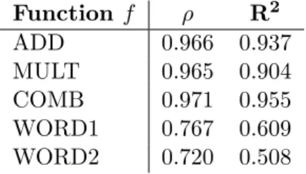
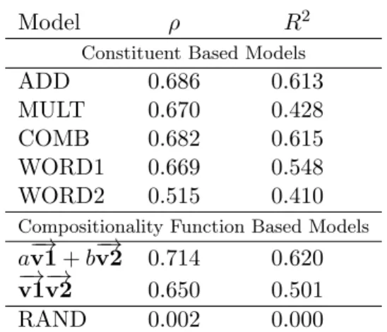
3.4 Correlations between functions and phrase compositionality scores . . . 47

3.5 Constituent level correlations . . . 51

3.6 Phrase level correlations of compositionality scores . . . 51

4.1 WSI parameter values. . . 61

4.2 Spearman Correlations of Model predictions with Human Pre-dictions . . . 67

5.1 APD and Acc on validation data . . . 76

5.2 Correlation Scores . . . 78

5.3 Average Point Difference Scores . . . 78

5.4 Coarse Grained Accuracy . . . 78

6.1 GPV metric results . . . 83

(14)

(15)

Declaration

I hereby declare that I composed this thesis entirely myself and it describes my own research.

Siva Reddy

University of York

Portions of this thesis are based on the following papers:

1. Siva Reddy, Ioannis P. Klapaftis, Diana McCarthy, Suresh Manand-har. Dynamic and Static Prototype Vectors for Semantic Composition. In Proceedings of The 5th International Joint Conference on Natural Language Processing 2011 (IJCNLP 2011), Chiang Mai, Thailand [Best Paper Award]

2. Siva Reddy, Diana McCarthy, Suresh Manandhar. An Empirical Study on Compositionality in Compound Nouns InProceedings of The 5th International Joint Conference on Natural Language Processing 2011 (IJCNLP 2011), Chiang Mai, Thailand

3. Siva Reddy, Diana McCarthy, Suresh Manandhar, Spandana Gella. Exemplar-based Word-Space Model for Compositionality Detection: Shared task system description. InProceedings of DISCo-2011 in con-junction with ACL-2011, 2011

[Our system was ranked 1st _{in two evaluation categories and}

2nd _{in two other]}

(16)

(17)

Chapter 1

Introduction

1.1 Compositional Semantics

How do humans comprehend utterances in natural language? How do we sum up the meaning of each component in an utterance and arrive at the right meaning? Can machines imitate this? While humans are highly com-petent in understanding multi word units like phrases, it still remains a herculean task for machines. Recent progress in semantic technologies like search engines has had an immense effect on human life, yet these technolo-gies are scratching the surface of human language at word level. The impact of semantic technologies at higher levels like phrases is far beyond the reach of existing systems. Potential applications include, but are not limited to: intelligent search engines, automatic answer grading, bio-medical applica-tions, question answering, textual entailment, and summarization.

Research in lexical semantics has made good progress in capturing individual word meanings. However, the same methods cannot be applied directly to model the semantics of phrases due to data sparsity. While vocabulary of a language is limited, its generative power for combinatorial expressions is nonrestrictive, and so lexical semantic methods fail to model phrasal or sentential semantics in-spite of how much ever data we use. Any model which aims capture language should be generative. But how do we make use of existing research in lexical semantics and advance further to phrasal or sentential semantics? The answer comes from Compositional Semantics.

(18)

18 1. Introduction

Compositional semantics involves the study of the meaning of an expression in relation with the meaning of its parts. ThePrinciple of Compositionality

[Pelletier, 1994, page. 313] states that the meaning of an expression is a

function of, and only of, the meaning of its parts and the way in which the parts are combined. While humans are gifted with this function, formaliz-ing its true mathematical structure will be a miracle, which is the goal of compositional models.

1.2 Challenges

Many factors such as the polysemy of constituent words, the role of syntactic structure, semantic preferences of constituents, idiomatic and metaphoric usages, play an important role in molding the meaning of an expression. Cracking the way in which humans process these components to arrive at a meaning will be a major breakthrough in computational linguistics. Below, we discuss some of the challenges in brief.

1.2.1 Polysemy of Constituent Words

Polysemy of words have been a major focus of lexical semantics. The chal-lenges posed at lexical level make a transition to phrasal and higher levels, making polysemy a major threat to compositional semantics. While the efforts of lexical sense disambiguation methods have not seen real benefits [Navigli, 2009], the effect of polysemy on compositional semantics is yet to be studied. Take an example phrase bank balance. In the WordNet [Fell-baum, 1998],bank andbalancehave 10 and 12 senses respectively. But, only one sense of bank and one sense of balance are relevant in the phrase bank balance, and choosing a correct sense for each constituent is critical for a good compositional model.

The questions, how do you make use of sense disambiguation? Is sense disambiguation really useful for compositional models?, still remains unan-swered and have to be explored.

(19)

1.2. Challenges 19 1.2.2 Syntactic Structure

The semantic interpretation of an expression changes with a change in its syntactic structure. For example, the semantics of phrases formed by the combinations of house and rent differ. The phrase house rent means the rent to be paid for a house whereas the phrase rent house means a house which is available on periodic rental basis. Syntactic structure guides the information flow in arriving at the correct interpretation of an expression. A good compositional model should take syntactic structure into account.

1.2.3 Semantic Preferences

Experimental studies on human sentence processing reveal that humans not only use lexical and syntactic information but also semantic preferences when processing a sentence [Pad´o et al., 2009]. For example, given an un-completed sentence such as“Among all the fruits, John likes to eat a/an ”, a human processing model starts expecting afruit in the blank, lets say or-ange. Perhaps the reasons for choosing orange is because the preferences of other words in the sentence expects an edible fruit and the properties of orange such as taste, juice, pulp makes it edible. Given that humans use semantic preferences in sentence processing, it is necessary for any good compositional model to take this information into consideration. Semantic preferences capture subtle properties beyond syntactic relations. For exam-ple, the semantic preferences of laser in the phrases laser light and laser treatment are different though the syntactic relation is the same (modifier). Inlaser light, the meaning gets transformed intoa specific type of light, and in laser treatment the meaning becomes a treatment using laser. In each phrase, the properties picked up due to semantic preferences of words are completely different. Semantic preferences of words help to choose relevant properties of words required for composition.

1.2.4 Idiomatic and Metaphoric usages

As the name compositional in compositional models indicate, compositional models are designed to build semantics compositionally from the meaning of their parts. But compositional interpretation may not be possible with

(20)

20 1. Introduction

idiomatic and metaphoric usages which are known to be non-compositional. In idiomatic expressions, the semantic interpretation of an expression is beyond the superficial meaning of its constituents e.g. he was born with a silver spoon, here the meaning of silver spoon is not literally meant but idiomatically meant to be rich. Most idioms can only be interpreted by knowing the meaning of the idiom beforehand. Metaphors on the other can be understood if one has enough cultural background e.g. Juliet is the sunshine in Romeo’s life, here it is meant Juliet means a lot to Romeo. It is uncertain if compositional models are expected to model the semantics of non-compositional expressions. However, a good compositional model should be able to distinguish compositional meaning from non-compositional meaning.

1.2.5 Other Challenges

Metonymy is a phenomenon in which a foreign word stands on behalf of a target word, the foreign word representing the semantics of the target word, e.g. everybody reads Shakespeare at school, here Shakespeare stands for his books rather than himself 1. Metonymy poses a major challenge to compositional semantics. In order to interpret metonymy, compositional models should make use of the clues from higher levels of semantic processing like discourse.

How do we formally represent semantics of words, phrases and text? Many frameworks exist for representing semantics. The most common ones in compositional semantics are formal semantics, and distributional semantics. Each framework has its own pros and cons. We will describe them in the coming sections. Depending on the framework we use, additional challenges creep in. We use distributional framework for all our compositional models, thus our research of interest is compositional distributional semantics. How do we make use of information from all the above sources and compose the semantics of an expression? Each semantic framework has its own way of using the above information. Composition functions are the most common which take constituent words and structure as input arguments, and the resultant semantic composition of the expression as the output.

(21)

1.3. What is thesis about? 21

The evaluation of compositional models is an uncertain topic. Since we hu-mans do not know the way we compose semantics of expressions, it is hard to prepare datasets for evaluation, thus making the evaluation of compo-sitional models a challenging topic. Most evaluation methods are external application-based.

1.3 What is thesis about?

In this thesis, we pursue some of the challenges described above. We aim to explore the effect of polysemy in compositional models. Our hypothe-sis is that sense disambiguation improves the performance of compositional models. Our focus is also on evaluation methods for compositional mod-els (Chapter 2). We create a compositionality dataset using Mechanical Turkers, and based on the dataset, we perform a study on the relation be-tween constituent words and phrase compositionality, revealing interesting facts about compositionality in language (Chapter 3). We evaluate sense disambiguation-based composition models using three evaluation methods, two application based and one an internal evaluation. We show improve-ments in performance due to sense disambiguation over standard models which do not perform disambiguation, thus validating our initial hypothesis (Chapter 4, 5, 6). Finally we discuss interesting findings from our observa-tions (Chapter 7).

1.4 Background

In this section we describe the background required to follow the upcoming chapters.

1.4.1 Representation of Semantics

In compositional semantics, two different frameworks have become popu-lar for representing semantics - (1) formal semantics and (2) distributional semantics.

(22)

22 1. Introduction

1.4.1.1 Formal Semantics

In formal semantics, semantics of an expression is represented in formal logic based on the grammatical structure while the meanings of words are sym-bolic with no rigid definition. According to Montague [1970] view of formal semantics, a human language can be modeled within a mathematically pre-cise theory. The advantage of formal semantics is its generative power. A formal semantic model can be represented by a grammar which translates (parses) a given expression into formal logic. Formal semantic models are known for their wide coverage.

The semantic representation of the sentenceevery man walks, according to Montague [1973], is defined as∀u[man(u) =⇒ walk(u)]. Some of the for-mal semantic methods include [Baldridge and Kruijff, 2002; Ge and Mooney, 2005; Copestake et al., 2005; Kate and Mooney, 2007; Chen and Mooney, 2008; Liang et al., 2011; Kwiatkowski et al., 2011]. Language processing applications can make use of formal representation and reason on it. The major drawback of formal representation is that it only deals with truth or falsity of meanings of an expression, but do not say anything about how to compare two different meanings. Formal semantic models deal more with syntax not worrying about lexical ambiguity. Since our focus is on lexical ambiguity, formal semantics is not our topic of interest in this thesis.

1.4.1.2 Distributional Semantics

Distributional hypothesis [Harris, 1954] states thatwords that occur in sim-ilar contexts tend to have simsim-ilar meanings. Firth [1957] states it as you shall know a word by the company it keeps. Distributional hypothesis is the backbone of statistical semantics, also called as distributional semantics. In distributional semantics, a word is represented by a distribution of its contexts. For a given word, the distribution of its contexts can be learned from the co-occurrence frequency of the contexts and the target word. Two words are said to be similar if they have similar distribution of contexts. For example,house and flat frequently occur with context words like rent, bedroom, sale etc, giving a clue to computational models that house and

(23)

1.4. Background 23

words in a fixed size window, their part-of-speech categories or the syntactic information or the combinations of any of these.

Similar to the representation of a word, an expression can be also repre-sented as a distribution of contexts. The goal of compositional distributional semantic models is to predict this distribution for an expression from the distributional representation of its constituents.

Ambiguity of words is well studied in distributional semantics. So we choose distributional framework to test our hypothesis. The most common imple-mentation of distributional models are vector space models (described in the next section).

The main advantage of distributional models is their ability to give a quan-titative assessment on the similarity between meanings. However, distribu-tional models are not generative like formal semantic models. It is highly challenging to encode structure of an expression into a distributional rep-resentation. It is also challenging to decode the structure of an expression from its distributional meaning.

1.4.2 Vector space model of meaning

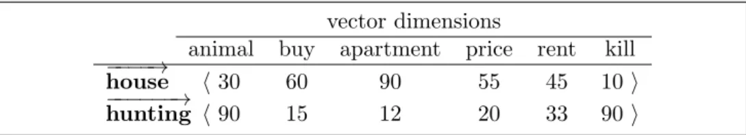
Vector Space Models (VSM) of distributional semantics [Turney and Pantel, 2010] have become a standard framework for representing a word’s meaning. Typically these methods [Sch¨utze, 1998; Pado and Lapata, 2007; Erk and Pad´o, 2008] utilize a bag-of-words model or syntactic dependencies such as subject/verb, object/verb relations, so as to extract the features which serve as the dimensions of the vector space. Each word is then represented as a vector of the extracted features, where the frequency of co-occurrence of the word with each feature is used to calculate the vector component associated with that feature. Phrases can also be represented as vectors by treating a phrasal unit to like a single word. Figure 1.1 provides a sample vector space representation of a phrase and its constituents assuming bag-of-words model.

Our VSM settings: The lemmatised context words along with their part of speech category around a target word in a window of size 100 are treated as its co-occurrences, e.g. evidence-n, fire-v etc. Concordances of words from

(24)

24 1. Introduction

vector dimensions

evidence-n memo-n health-n pistol-n fire-v

−−−−−−→ smoking h9 2 181 4 37i −−→ gun h10 3 5 98 270i −−−−−−−−−−→ smoking gun h83 33 6 0 6i

Figure 1.1: Co-occurrence vectors ofsmoking gun and its constituents

ukWaC corpus [Ferraresi et al., 2008] are used to compute co-occurrence frequencies of context words. The top 10000 frequent content words in ukWaC corpus (along with their part-of-speech category) are only treated as co-occurrences i.e. the vector dimensions. Vector of a word is built from its concordances in ukWaC. To measure the similarity between two vectors, we use cosine similarity (sim).

sim(−v1→,−v2→) =

−→

v1·−v2→

||−v1→|| ||−v2→||

Following Mitchell and Lapata [2008], the context words in the vector are set to the ratio of probability of the context word given the target word to the overall probability of the context word2.

1.4.3 Compositional Distributional Semantics

Compositional Distributional Semantics (CDS) models deal with the task of composing the meaning of a phrase/sentence from the distributional mean-ing of its constituents and the structure. These models define composition function (⊕), which takes constituent word vectors and structure as input, and gives the resultant semantic composition as output. Below, we discuss some of the composition functions.

Mitchell and Lapata [2008]use simple addition and simple multiplication of constituent word vectors to compose phrasal semantics. For example, for the phrasehouse hunting

• Simple addition: ⊕(house hunting) = a−−−−→house + b−−−−−−→hunting wherea and b are scalars.

(25)

1.4. Background 25

• Simple multiplication: ⊕(house hunting) =

−−−−→

house −−−−−−→hunting where

⊕(house hunting)i =

−−−−→

housei *

−−−−−−→

huntingi

The resulting composition does not take structure into account, e.g. −−−−→house⊕ −−−−−−→

hunting looks the same as−−−−−−→hunting⊕−−−−→house (if a=b).

The background should be enough by now to understand the rest of the thesis. Readers can skip to Chapter 2. Interested readers on composition functions may proceed.

Erk and Pad´o [2008] make the above model structure sensitive by using selectional preferences of constituents. Figure 1.2 displays the composition procedure. To compose the semantics of the phrase −−−→catch←obj−−−→ball, the semantic preference vector of catch formed by all its objects filter the contexts of−−→ball, and similarly the semantic preference vector ofball formed by all its inverse objects filter the contexts of −−−→catch, and these filtered vectors are used for composition. In this setting, the composition of house hunting andhunting house differs.

Widdows [2008]use tensor product to account for word order. The com-position of house hunting is defined as

⊕(house hunting) =P i,j −−−−→ housei∗ −−−−→ housej [ −−−−→ housei× −−−−−−→ huntingi]

If the initial vector space is n-dimensional, the resultant vector space of

⊕(house hunting) isn2 dimensions.

Guevara [2010] propose additive and multiplicative models which look slightly similar to [Mitchell and Lapata, 2008].

• Additive Model: ⊕(house hunting) = A −−−−→house +B −−−−−−→hunting where

A andB are matrices.

• Multiplicative Model: ⊕(house hunting) =A

−−−−→

house −−−−−−→hunting, where A is a matrix.

The matrices account for structure making the composition word order sen-sitive.

(26)

syn-26 1. Introduction

Figure 1.2: Composition using Structured vector space model. Courtesy: [Erk and Pad´o, 2008]

tactic relation between words is represented using a neural network (sigmoid-like function) which takes argument word vectors as input, and gives the resultant phrase composition vector as output.

Clark and Pulman [2007]aim to capture structure of a phrase/sentence by representing compositional meaning in a higher-order dimensional space using tensor product operation⊗. Take an example sentence“the boy ate a juicy orange”. The structure can be represented asboy –subj→ ate ←obj–

orange←mod– juicy. Composition of this sentence is defined as:

−−→

boy⊗−−−→subj⊗(−→ate⊗obj−−→⊗(−−−→juicy⊗−−−→mod⊗ −−−−−→orange))

Sentences with different lengths are located in different higher-order dimen-sional spaces making it infeasible to measure the similarity between two unequal sentences. Dimensions of the space increase exponentially with in-crease in sentence length. The vector representation of a dependency relation is unclear. There is no experimental implementation of this work yet.

Grefenstette and Sadrzadeh [2011]assume that words belong to differ-ent type-based categories, and differdiffer-ent categories exist in differdiffer-ent dimen-sional spaces. The category of a word is decided by the number of adjoints

(27)

1.4. Background 27

(arguments) it can take. The composition of a sentence results in a final vector which exists in sentential space. The vectors of verbs, adjectives and adverbs act as relational functions which modify the properties of noun vectors. For example, “the boy ate a juicy orange” results in a composition

−→

ate⊙(−−→boy⊗(−−−→juicy⊙ −−−−−→orange))

where ⊙ is point-wise multiplication acting as a filtering operator and ⊗

is a tensor operator which is taking structure (order) into consideration. The above equation can be interpreted as: The selectional preferences of the relational words (here ate, and juicy) are filtering the noise in their corresponding arguments (nouns).

Let the category of a noun be n. Noun is assumed not to demand any arguments. The category of a relational word (verb, adjective, adverb) is decided by the number of arguments (adjoints) it takes and the category of the resultant output after combining with its arguments. For example, the adjoint of an adjective is noun (nr) (located right) and the category after combining with noun is a nounn (adjective combines with a noun resulting in a noun(-phrase)). So the category isadj=nnr. Similarly, lets say a verb can take at most two adjoints one on the left (subjnl_{) and one on the right}

(object nr), and the category of the output when the verb is combined with subject and object is a sentence s. So the category of verb is defined as

v =nl_snr_{. Similarly category of an adverb is} _adv ₌_vl_v_{. These categories}

decide the vector space in which corresponding words live.

All the resulting sentential vectors exist in the same space which is remark-able. However, the main limitations are

• As the number of adjoints of a word increase, the space in which it lives increases exponentially.

• It is always a prerequisite to have a verb to compute sentential seman-tics.

• The method is not designed for phrases.

• Similarity between words in different categories cannot be computed since they exist in different vector spaces e.g. the noun running and the verb run.

(28)

(29)

Chapter 2

Evaluation Methods

The aim of CDS models is to predict the semantics or the semantic behavior of the phrase from the constituents. But how do we say the predictions are correct? To date, the evaluation of CDS models is still a very uncertain issue. In this chapter, we give an overview of existing evaluation methods, their advantages and limitations.

There have been multiple proposals on evaluating CDS models. Most of them evaluate semantic behavior of the phrase rather than the evaluating the predicted semantics. Semantic behavior is evaluated on the basis of models’ performance in reproducing human annotations on external tasks. Evaluating the predicted semantics require a comparison with the true se-mantics. The true semantics of phrases is not straightforward to capture, after all the goal of CDS is to predict this. However, distributional rep-resentation of the phrase obtained from a large corpus gives us an idea of its true semantics. CDS models are evaluated on their ability to reproduce this distributional representation observed from a corpus. This evaluation is considered to be an internal evaluation task.

External evaluation tasks include, but are not limited to, paraphrasing, compositionality detection, lexical substitution, summarization. Recently, a couple of these tasks have been integrated into a single shared task, and is being organized as a SemEval 2013 shared task 1.

In the followings sections, we describe three evaluation methods which are

1_{http://www.cs.york.ac.uk/semeval-2013/task5/}

(30)

30 2. Evaluation Methods

Annotator N N’ rating

4 phone call committee meeting 2 25 phone call committee meeting 7 11 football club league match 6 11 health service bus company 1 14 company director assistant manager 7

Table 2.1: Evaluation dataset of [Mitchell and Lapata, 2010]

of particular interest to us.

2.1 Paraphrasing or Phrasal Similarity

Given a phrase, paraphrasing is the task of choosing alternative phrases which are similar to the given phrase. Paraphrasing datasets are prepared by human annotators. Humans generate paraphrases of a given phrase and also rank them based on the similarity with the given phrase. A good CDS model should correlate well with human rankings of paraphrases. The task can also be called as phrasal similarity task.

Mitchell and Lapata [2010] prepared a dataset which contains pairs of com-pound nouns and their similarity judgments. The dataset consists of 108 compound noun pairs with each pair having 7 annotations from different annotators who judge the pair for similarity in the range of score 1-7. A sample of 5 compound pairs is displayed in Table 2.1.

For each pair of the compound nouns, we take the mean value of all its human annotations as the final similarity judgment of the compound. LetN andN′

be a pair. To evaluate a model, we calculate the cosine similarity between the composed vectors −−−→⊕(N) and −−−−→⊕(N′) obtained from the composition, where

⊕() denotes composition function. These similarity scores are correlated with human mean scores to judge the performance of a model. Higher the correlation, better is the CDS model.

Mitchell and Lapata [2008] also prepared a similar dataset for subject-verb phrases. Each phrase is paired with two landmark verbs, the synonyms of the reference verb in the phrase. The landmarks represent distinct word senses of the reference verb, one compatible with the reference phrase and the other incompatible e.g, forThe face glowed, the landmarks burned and

(31)

2.1. Paraphrasing or Phrasal Similarity 31

Noun Reference High Low The fire glowed burned beamed The face glowed beamed burned The child strayed roamed digressed The discussion strayed digressed roamed The sales slumped declined slouched The shoulders slumped slouched declined

Table 2.2: Example Stimuli with High and Low similarity landmarks. Cour-tesy: Mitchell and Lapata [2008]

beamed are synonyms ofglowed representing different senses ofglowed while

beamed is compatible with the reference phrase,burned is incompatible. A good CDS model should be able to compose the semantics of the phrase such that the phrasal vector is similar (closer) to the high-similarity landmark and different (farther) to the low-similarity landmark. Table 2.2 displays a sample from [Mitchell and Lapata, 2008] dataset.

In SemEval-2013, a shared task calledIdentifying semantically similar phrases in context is being organized based on idea of paraphrasing. For a given phrase, the participating systems should predict best similar phrases from very large corpora. Later, these phrases will be ranked by humans for phrase similarity. The evaluation method is kind-of reverse program to [Mitchell and Lapata, 2010].

The advantages of all the above methods in this evaluation are

• Since the final goal is only to predict or rank similar phrases of a given phrase, the evaluation method is independent of the dimensional space used by the CDS models.

• The evaluation method is easy to interpret and have many practical applications in natural language generation.

While the disadvantages are

• The evaluation is “external” since the actual composition task is not evaluated but evaluated on a different task.

• The evaluation method involves human annotations making the task expensive.

(32)

2.2 Compositionality Detection

A phrase is compositional if its meaning can be interpreted from the meaning of its constituents e.g. swimming pool. Not all phrases in a language are compositional. For example, the meaning ofcouch potatois hard to interpret from the meaning ofcouch andpotato. Such phrases are non-compositional. Some phrases fall in-between compositional and non-compositional e.g. rush hour. The task of compositionality detection involves in identifying phrases which are compositional and non-compositional2.

It is unclear if compositional models are expected to compose the semantics of non-compositional phrases. Pelletier [1994] presents arguments in favor of and against the notion of compositional models (compositionality principle) modeling the semantics of non-compositional phrases. Many existing meth-ods [Schone and Jurafsky, 2001; Baldwinet al., 2003; Giesbrecht, 2009] for compositionality detection assume compositional meaning from CDS mod-els is completely different from non-compositional meaning. If a phrase is non-compositional, a good CDS model should compose the semantics of the phrase such that it is father from its actual meaning. If the phrase is com-positional, the composition should lead to a meaning closer to the actual meaning. Based on this assumption, CDS models are evaluated on compo-sitionality detection tasks.

In this evaluation, human annotate datasets with compositionality judg-ments. CDS models are evaluated based on their ability in reproducing human compositionality judgments of the annotated phrases. Recently Bie-mann and Giesbrecht [2011] organized a shared task based on the composi-tionality detection criteria.

There are many existing datasets marked with compositionality judgments. All the existing datasets are type-based evaluation datasets and are not context based evaluations. For example,red carpet have both compositional and non-compositional meaning. Type-based evaluation datasets are an-notated only for the most frequent compositional behavior of the phrase (and thereforered carpet is non-compositional) and not context-dependent variation (InThe floor is covered with red carpet,red carpet is

com-2_{For a deeper linguistic classification of phrases (multiwords), please refer to [Sag} _et al., 2002]

(33)

2.3. Similarity with Gold Phrasal Vectors (GPV metric) 33

positional). In SemEval 2013, a shared task is proposed on the idea of context-based evaluation of compositionality.

Existing type-based evaluation datasets either classify phrases into differ-ent classes or have scores demonstrating the degree of composition. Ban-nardet al. [2003] found moderate inter-annotator agreements in classifying the compounds into discrete classes, depicting the task is hard even for humans. Instead, McCarthy et al. [2003] suggests that compositionality exhibits a continuum, and created a dataset marked with compositionality scores rather than discrete classes.

In the next chapter, we discuss about existing type-based evaluation datasets and point out their limitations. We propose an annotation scheme differ-ent from the existing approaches and create a compositionality dataset for compound nouns. Our dataset is found to exhibit the continuum of compo-sitionality.

The advantages of compositionality detection based evaluations are

• CDS models are evaluated both for compositionality and non-compositionality. • The evaluation method is independent of the dimensional space used

by the CDS models.

• The task may lead to creating better language understanding models. However, the main disadvantages are

• The task is hard even for humans to classify phrases into compositional and non-compositional.

• The dataset is expensive to prepare.

• The evaluation is “external” since CDS models are evaluated on a task different to the actual task.

2.3 Similarity with Gold Phrasal Vectors (GPV

metric)

In this evaluation metric, we evaluate compositional models by measuring the similarity between the distributional vector of a phrase built from the

(34)

corpus (Gold Phrasal Vectors) and the composed vector predicted by the models. A similar evaluation metric is proposed by Guevara [2011]. The evaluation is considered an internal evaluation metric since the evaluation is assessing the performance of CDS models on the actual semantic compo-sition task and not an external task.

Given a set of n phrases, gold distributional vectors −→G1, −→G2 . . . of the phrases are constructed using corpus instances of the phrases by treating the phrase as a single word unit, similar to building constituent word vectors. LetAandB be two CDS models. CDS modelAis said to be better thanB, ifA’s composed vectors −→A1, −→A2. . . of the given phrases are closer to −→G1,

−→

G2. . . thanB’s composed vectors −→B1,−→B2. . .. Leta1, a2 . . ., where ai =sim(

−→

Ai,−Gi→), be the cosine similarities of model

A’s composed vectors and gold vectors. Similarly, b1, b2 . . ., where bi = sim(−Bi→,−Gi→), be the cosine similarities of model B’s composed vectors and gold vectors. Model A performance is measured by calculating its overall similarity defined as

GP V(A) =

Pn

1ai n

Similarly Model B’s overall similarity is defined as GP V(B) =

Pn 1bi n . The

model which gives higher overall similarity is a better compositional model than the one which gives lower similarity score. An ideal model should give an overall similarity score of 1.

The advantages of this model are

• The method does not require human annotated data, thus is less ex-pensive and faster to create.

• “Internal” evaluation metric which evaluates the actual task. However, the limitations are

• The method is badly affected by data sparsity as the length of the phrase increases.

• The method does not work for low frequency phrases even if the phrasal length is small.

(35)

2.4. Summary 35

• The predicted compositional vector should exist in the same space, thereby restricting the semantic composition functions that can be used.

• Method cannot be applied to phrases which do not occur in general language.

• It is unclear how to evaluate non-compositional phrases

2.4 Summary

In the above sections we discussed evaluation methods for CDS models and described three such methods in detail. There is no hard-and-fast rule in choosing an evaluation method. It mainly depends on the implementation of the CDS model and the task of interest. For example, GPV metric (Section 2.3) cannot be used if the composition vectors exist in different dimensional space than the gold vectors. In the coming chapters, we use the above mentioned evaluation methods to evaluate our CDS models.

In the next chapter we discuss the evaluation metric Compositionality De-tection in detail. We propose a new annotation scheme for annotating com-positionality judgments, describe an experimental setup for collecting an-notations from many annotators, and evaluate computational methods for compositionality detection on our dataset.

(36)

(37)

Chapter 3

An Empirical Study on

Compositionality

In the previous chapter we introducedcompositionality detectionevaluation method (Section 2.2). In this chapter, we collect and analyze the com-positionality judgments for a range of compound nouns using Mechanical Turk to create a new compositionality detection dataset. Unlike existing compositionality datasets, our dataset has judgments on the contribution of constituent words as well as judgments for the phrase as a whole. We use this dataset to study the relation between the judgments at constituent level to that for the whole phrase. We introduce simple models of compositionality detection and evaluate them on our new dataset.

The past decade has seen interest in developing computational methods for compositionality detection [Lin, 1999; Schone and Jurafsky, 2001; Baldwin

et al., 2003; Bannard et al., 2003; McCarthyet al., 2003; Venkatapathy and Joshi, 2005; Katz and Giesbrecht, 2006; Sporleder and Li, 2009]. Recent developments in vector-based semantic composition functions [Mitchell and Lapata, 2008; Widdows, 2008] have also been applied to compositionality detection [Giesbrecht, 2009]. All these methods use constituent word seman-tics in contrast with the phrasal semanseman-tics to determine the compositionality of the phrase.

While the existing methods of compositionality detection use constituent word level semantics, the evaluation datasets are not particularly suitable

(38)

38 3. An Empirical Study on Compositionality

to study the contribution of each constituent word to the semantics of the phrase. Existing datasets [McCarthy et al., 2003; Venkatapathy and Joshi, 2005; Katz and Giesbrecht, 2006; Biemann and Giesbrecht, 2011] only have the compositionality judgment of the whole expression without constituent word level judgment, or they have judgments on the constituents without judgments on the whole [Bannard et al., 2003]. Our dataset allows us to examine the relationship between the two rather than assume the nature of it.

We collect judgments of the contribution of constituent nouns within noun-noun compounds (Section 3.1) alongside judgments of compositionality of the compound. We study the relation between the contribution of the parts with the compositionality of the whole (Section 3.2). We propose various constituent based models (Section 3.3.2) which are intuitive and related to existing models of compositionality detection (Section 3.3.1) and we evaluate these models in comparison to composition function based models. All the models discussed in this chapter are built using a distributional word-space model approach [Sahlgren, 2006].

3.1 Compositionality in Compound Nouns

In this section, we describe the experimental setup for the collecting compo-sitionality judgments of English compound nouns. All the existing datasets focused either on verb-particle, verb-noun or adjective-noun phrases. In-stead, we focus oncompound nounsfor which resources are relatively scarce. In this chapter, we only deal with compound nouns made up of two words separated by space.

3.1.1 Annotation setup

In the literature [Nunberg et al., 1994; Baldwin et al., 2003; Fazly et al., 2009], compositionality is discussed in many terms including simple decom-posable, semantically analyzable, idiosyncratically decomposable and non-decomposable. For practical NLP purposes, Bannard et al. [2003] adopt a straightforward definition of a compound being compositional if“the overall semantics of the multi-word expression (here compound) can be composed

(39)

3.1. Compositionality in Compound Nouns 39 from the simplex semantics of its parts, as described (explicitly or implic-itly) in a finite lexicon”. We adopt this definition and pose compositionality as a literality issue. A compound is compositional if its meaning can be understood from the literal (simplex) meaning of its parts. Similar views of compositionality as literality are found in [Lin, 1999; Katz and Giesbrecht, 2006]. In the past there have been arguments in favor/disfavor of composi-tionality as literality approach (e.g. see [Gibbs, 1989; Titone and Connine, 1999]). The idea of viewing compositionality as literality is also motivated from the shared task organized by Biemann and Giesbrecht [2011]. From here on, we use the terms compositionality and literality interchangeably. We ask humans to score the compositionality of a phrase by asking them

how literal the phrase is. Since we wish to see in our data the extent that the phrase is compositional, and to what extent that depends on the contribution in meaning of its parts, we also ask themhow literal the use of a component word is within the given phrase.

For each compound noun, we create three separate tasks – one for each con-stituent’s literality and one for the phrase compositionality. Tasks for the compound noun “sacred cow” are displayed in the Figure 3.1. The moti-vation behind using three separate tasks is to make the scoring mechanism for each task independent of the other tasks. This enables us to study the actual relation between the constituents and the compound scores without any bias to any particular annotator’s way of arriving at the scores of the compound w.r.t. the constituents.

There are many factors to consider in eliciting compositionality judgments, such as ambiguity of the expression and individual variation of annotator in background knowledge. To control for this, we ask subjects if they can interpret the meaning of a compound noun from only the meaning of the component nouns where we also provide contextual information. All the possible definitions of a compound noun are chosen from WordNet [Fell-baum, 1998], Wiktionary or defined by ourselves if some of the definitions are absent. Five examples of each compound noun are randomly chosen from the ukWaC [Ferraresiet al., 2008] corpus and the same set of examples are displayed to all the annotators. The annotators select the definition of the compound noun which occurs most frequently in the examples and then score the compound for literality based on the most frequent definition.

(40)

Phrase: sacred cow

Definitions:

1. a person unreasonably held to be immune to criticism 2. A cow which is worshipped

Examples:

1. we told our director , Kenneth Loach , that none of thesacred cows of television drama need stand in his way

2. Meles Zenawi said in an interview that there were no sacred cows in a war on corruption

3. many of thesacred cowswill have to be sacrificed to fund digitization

4. you will find any number ofsacred cows which are regarded as an intrinsic part of the teachings. Think of reincarnation, chakras, karma

5. TOTP has finally become the latestsacred cow to be slaughtered by the BBC

Instructions:

• Select the definition of sacred cow which occurs most of the times in the above examples. Ignore other definitions. Based on the definition chosen, score below tasks

• Scoring guidelines: Enter a number between 0 and 5

– 0 means: Not to be understood literally at all

– 5 means: To be understood very literally

– Use values in between to grade your decision

Note: Each task below is dispalyed separately to different annotators.

Task1: Score of 0-5 for how literal is the phrasesacred cow

Task2: Score of 0-5 for how literal is the use ofsacred in the phrasesacred cow

Task3: Score of 0-5 for how literal is the use ofcow in the phrasesacred cow

Figure 3.1: Sample annotation tasks for sacred cow

We have two reasons for making the annotators read the examples, choose the most frequent definition and base literality judgments on the most fre-quent definition. The first reason is to provide a context to the decisions and reduce the impact of ambiguity. The second is that distributional models are greatly influenced by frequency and since we aim to work with distri-butional models for compositionality detection we base our findings on the most frequent sense of the compound noun. In this work we consider the compositionality of the noun-noun compound type without token based dis-ambiguation which we leave for future work.

3.1.2 Compound noun dataset

We could not find any compound noun datasets publicly available which are marked for compositionality judgments. Korkontzelos and Manandhar [2009] prepared a related dataset for compound nouns but

(41)

compositional-3.1. Compositionality in Compound Nouns 41

ity scores were absent and their set contains only 38 compounds. There are datasets for verb-particle [McCarthyet al., 2003], verb-noun judgments [Bie-mann and Giesbrecht, 2011; Venkatapathy and Joshi, 2005] and adjective-noun [Biemann and Giesbrecht, 2011]. Not only are these not the focus of our work, but also we wanted datasets with each constituent word’s literality score. Bannardet al. [2003] obtained judgments on whether a verb-particle construction implies the verb or the particle or both. The judgments were binary and not on a scale and there was no judgment of compositionality of the whole construction. Ours is the first attempt to provide a dataset which have both scalar compositionality judgments of the phrase as well as the literality score for each component word.

We aimed for a dataset which would include compound nouns where: 1) both the component words are used literally, 2) the first word is used literally but not the second, 3) the second word is used literally but not the first and 4) both the words are used non-literally. Such a dataset would provide stronger evidence to study the relation between the constituents of the compound noun and its compositionality behaviour.

We used the following heuristics based on WordNet to classify compound nouns into 4 above classes.

1. Each of the component word exists either in the hypernymy hierarchy of the compound noun or in the definition(s) of the compound noun. e.g. swimming pool because swimming exists in the WordNet defini-tion of swimming pool and pool exists in the hypernymy hierarchy of

swimming pool

2. Only the first word exists either in the hypernymy hierarchy or in the definition(s) of the compound and not the second word. e.g. night owl

3. Only the second word exists either in the hypernymy hierarchy or in the definition(s) of the compound and not the first word. e.g. zebra crossing

4. Neither of the words exist either in hypernymy hierarchy or in the definition(s) of the compound noun. e.g. smoking gun

The intuition behind the heuristics is that if a component word is used literally in a compound, it would probably be used in the definition of the compound or may appear in the synset hierarchy of the compound. We

(42)

changed the constraints, for example decreasing/increasing the depth of the hypernymy hierarchy, and for each class we randomly picked 30 potential candidates by rough manual verification. There were fewer instances in the classes 2 and 4. In order to populate these classes, we selected additional compound nouns from Wiktionary by manually inspecting if they can fall in either class.

These heuristics were only used for obtaining our sample, they werenot used for categorizing the compound nouns in our study. The compound nouns in all these temporary classes are merged and 90 compound words are selected which have at least 50 instances in the ukWaC corpus. These 90 compound words are chosen for the dataset.

3.1.3 Annotators

Snow et al. [2008] used Amazon mechanical turk (AMT) for annotating language processing tasks. They found that although an individual turker (annotator) performance was lower compared to an expert, as the number of turkers increases, the quality of the annotated data surpassed expert level quality. We used 30 turkers for annotating each single task and then retained the judgments with sufficient consensus as described in Section 3.1.4. For each compound noun, 3 types of tasks are created as described above: a judgment on how literal the phrase is and a judgment on how literal each noun is within the compound. For 90 compound nouns, 270 independent tasks are therefore created. Each of these tasks is assigned to 30 annotators. A task is assigned randomly to an annotator by AMT so each annotator may work on only some of the tasks for a given compound.

3.1.4 Quality of the annotations

Recent studies1 shows that AMT data is prone to spammers and outliers. We dealt with them in three ways. a). We designed a qualification test2 which provides an annotator with basic training about literality, and they

1_{A study on AMT spammers}_{http://bit.ly/e1IPil}

2_{The qualification test details are provided with the dataset. Please refer to footnote} 3.

(43)

3.1. Compositionality in Compound Nouns 43

No. of turkers participated 260

No. of them qualified 151

Turkers withρ <= 0 21 Turkers withρ >= 0.6 81 No. of annotations rejected 383 Avg. submit time (sec) per task 30.4

highestρ avg. ρ ρfor phrase compositionality 0.741 0.522

ρfor first word’s literality 0.758 0.570

ρfor second word’s literality 0.812 0.616

ρfor over all three task types 0.788 0.589

Table 3.1: Amazon Mechanical Turk statistics

can participate in the annotation task only if they pass the test. b). Once all the annotations (90 phrases * 3 tasks/phrase * 30 annotations/task = 8100 annotations) are completed, we calculated the average Spearman correlation score (ρ) of every annotator by correlating their annotation values with every other annotator and taking the average. We discarded the work of annotators whose ρ is negative and accepted all the work of annotators whoseρis greater than 0.6. c). For the other annotators, we accepted their annotation for a task only if their annotation judgment is within the range of ±1.5 from the task’s mean. Table 3.1 displays AMT statistics. Overall, each annotator on average worked on 53 tasks randomly selected from the set of 270 tasks. This lowers the chance of bias in the data because of any particular annotator.

Spearman correlation scores ρ provide an estimate of annotator agreement. To know the difficulty level of the three types of tasks described in Section 3.1, ρ for each task type is also displayed in Table 3.1. It is evident that annotators agree more at word level than phrase level annotations. Thus, providing literality scores at component word level is an additional advan-tage of our dataset compared to the existing datasets on compositionality judgments.

For each compound, we also studied the distribution of scores around the mean by observing the standard deviationσ. All the compound nouns along with their mean and standard deviations are shown in Table 3.2.

Ideally, if all the annotators agree on a judgment for a given compound or a component word, the deviation should be low. Among the 90 compounds, 15 of them are found to have a deviation>±1.5. These are displayed in Table

(44)

Compound Word1 Word2 Phrase Compound Word1 Word2 Phrase

climate change 4.90±_0.30 _4.83±_0.38 _4.97±_0.18 _{engine room} _4.86±_0.34 _5.00±_0.00 _4.93±_0.25

graduate student 4.70±_0.46 _5.00±_0.00 _4.90±_0.30 _{swimming pool} _4.80±_0.40 _4.90±_0.30 _4.87±_0.34

speed limit 4.93±_0.25 _4.83±_0.38 _4.83±_0.46 _{research project} _4.90±_0.30 _4.53±_0.96 _4.82±_0.38

application form 4.77±_0.42 _4.86±_0.34 _4.80±_0.48 _{bank account} _4.87±_0.34 _4.83±_0.46 _4.73±_0.44

parking lot 4.83±_0.37 _4.77±_0.50 _4.70±_0.64 _{credit card} _4.67±_0.54 _4.90±_0.30 _4.67±_0.70

ground floor 4.66±_0.66 _4.70±_0.78 _4.67±_0.60 _{mailing list} _4.67±_0.54 _4.93±_0.25 _4.67±_0.47

call centre 4.73±_0.44 _4.41±_0.72 _4.66±_0.66 _{video game} _4.50±_0.72 _5.00±_0.00 _4.60±_0.61

human being 4.86±_0.34 _4.33±_1.14 _4.59±_0.72 _{interest rate} _4.34±_0.99 _4.69±_0.53 _4.57±_0.90

radio station 4.66±_0.96 _4.34±_0.80 _4.47±_0.72 _{health insurance} _4.53±_0.88 _4.83±_0.58 _4.40±_1.17

law firm 4.72±_0.52 _3.89±_1.50 _4.40±_0.76 _{public service} _4.67±_0.65 _4.77±_0.62 _4.40±_0.76

end user 3.87±_1.12 _4.87±_0.34 _4.25±_0.87 _{car park} _4.90±_0.40 _4.00±_1.10 _4.20±_1.05

role model 3.55±_1.22 _4.00±_1.03 _4.11±_1.07 _{head teacher} _2.93±_1.51 _4.52±_1.07 _4.00±_1.16

fashion plate 4.41±_1.07 _3.31±_2.07 _3.90±_1.42 _{balance sheet} _3.82±_0.89 _3.90±_0.96 _3.86±_1.01

china clay 2.00±_1.84 _4.62±_1.00 _3.85±_1.27 _{game plan} _2.82±_1.96 _4.86±_0.34 _3.83±_1.23

brick wall 3.16±_2.20 _3.53±_1.86 _3.79±_1.75 _{web site} _2.68±_1.69 _3.93±_1.18 _3.79±_1.21

brass ring 3.73±_1.95 _3.87±_1.98 _3.72±_1.84 _{case study} _3.66±_1.12 _4.67±_0.47 _3.70±_0.97

polo shirt 1.73±_1.41 _5.00±_0.00 _3.37±_1.38 _{rush hour} _3.11±_1.37 _2.86±_1.36 _3.33±_1.27

search engine 4.62±_0.96 _2.25±_1.70 _3.32±_1.16 _{cocktail dress} _1.40±_1.08 _5.00±_0.00 _3.04±_1.22

face value 1.39±_1.11 _4.64±_0.81 _3.04±_0.88 _{chain reaction} _2.41±_1.16 _4.52±_0.72 _2.93±_1.14

cheat sheet 2.30±_1.59 _4.00±_0.83 _2.89±_1.11 _{blame game} _4.61±_0.67 _2.00±_1.28 _2.72±_0.92

fine line 3.17±_1.34 _2.03±_1.52 _2.69±_1.21 _{front runner} _3.97±_0.96 _1.29±_1.10 _2.66±_1.32

grandfather clock 0.43±_0.78 _5.00±_0.00 _2.64±_1.32 _{lotus position} _1.11±_1.17 _4.78±_0.42 _2.48±_1.22

spelling bee 4.81±_0.77 _0.52±_1.04 _2.45±_1.25 _{silver screen} _1.41±_1.57 _3.23±_1.45 _2.38±_1.63

smoking jacket 1.04±_0.82 _4.90±_0.30 _2.32±_1.29 _{spinning jenny} _4.67±_0.54 _0.41±_0.77 _2.28±_1.08

number crunching 4.48±_0.77 _0.97±_1.13 _2.26±_1.00 _{guilt trip} _4.71±_0.59 _0.86±_0.94 _2.19±_1.16

memory lane 4.75±_0.51 _0.71±_0.80 _2.17±_1.04 _{crash course} _0.96±_0.94 _4.23±_0.92 _2.14±_1.27

rock bottom 0.74±_0.89 _3.80±_1.08 _2.14±_1.19 _{think tank} _3.96±_1.06 _0.47±_0.62 _2.04±_1.13

night owl 4.47±_0.88 _0.50±_0.82 _1.93±_1.27 _{panda car} _0.50±_0.56 _4.66±_1.15 _1.81±_1.07

diamond wedding 1.07±_1.29 _3.41±_1.34 _1.70±_1.05 _{firing line} _1.61±_1.65 _1.89±_1.50 _1.70±_1.72

pecking order 0.78±_0.92 _3.89±_1.40 _1.69±_0.88 _{lip service} _2.03±_1.25 _1.75±_1.40 _1.62±_1.06

cash cow 4.22±_1.07 _0.37±_0.73 _1.56±_1.10 _{graveyard shift} _0.38±_0.61 _4.50±_0.72 _1.52±_1.17

sacred cow 1.93±_1.65 _0.96±_1.72 _1.52±_1.52 _{silver spoon} _1.59±_1.47 _1.44±_1.77 _1.52±_1.45

flea market 0.38±_0.81 _4.71±_0.84 _1.52±_1.13 _{eye candy} _3.83±_1.05 _0.71±_0.75 _1.48±_1.10

rocket science 0.64±_0.97 _1.55±_1.40 _1.43±_1.35 _{couch potato} _3.27±_1.48 _0.34±_0.66 _1.41±_1.03

kangaroo court 0.17±_0.37 _4.43±_1.02 _1.37±_1.05 _{snail mail} _0.60±_0.80 _4.59±_1.10 _1.31±_1.02

crocodile tears 0.19±_0.47 _3.79±_1.05 _1.25±_1.09 _{cutting edge} _0.88±_1.19 _1.73±_1.63 _1.25±_1.18

zebra crossing 0.76±_0.62 _4.61±_0.86 _1.25±_1.02 _{acid test} _0.71±_1.10 _3.90±_1.24 _1.22±_1.26

shrinking violet 2.28±_1.44 _0.23±_0.56 _1.07±_1.01 _{sitting duck} _1.48±_1.48 _0.41±_0.67 _0.96±_1.04

rat race 0.25±_0.51 _2.04±_1.32 _0.86±_0.99 _{swan song} _0.38±_0.61 _1.11±_1.14 _0.83±_0.91

gold mine 1.38±_1.42 _0.70±_0.81 _0.81±_0.82 _{rat run} _0.41±_0.62 _2.33±_1.40 _0.79±_0.66

nest egg 0.79±_0.98 _0.50±_0.87 _0.78±_0.87 _{agony aunt} _1.86±_1.22 _0.43±_0.56 _0.76±_0.86

snake oil 0.37±_0.55 _0.81±_1.25 _0.75±_1.12 _{monkey business} _0.67±_1.01 _1.85±_1.30 _0.72±_0.69

smoking gun 0.71±_0.75 _1.00±_0.94 _0.71±_0.84 _{silver bullet} _0.52±_1.00 _0.55±_1.10 _0.67±_1.15

melting pot 1.00±_1.15 _0.48±_0.63 _0.54±_0.63 _{ivory tower} _0.38±_1.03 _0.54±_0.68 _0.46±_0.68

cloud nine 0.47±_0.62 _0.23±_0.42 _0.33±_0.54 _{gravy train} _0.30±_0.46 _0.45±_0.77 _0.31±_0.59

Table 3.2: Compounds with their constituent and phrase level mean±deviation scores

(45)

3.1. Compositionality in Compound Nouns 45

brass ring brick wall cheat sheet china clay cutting edge fashion plate fine line firing line game plan head teacher sacred cow silver screen search engine silver spoon web site

Table 3.3: Ambiguous Compounds withσ >±1.5

0 1 2 3 4 5 0 15 30 45 60 75 90 Compositionality Scores Compound Nouns

Figure 3.2: Mean values of phrase-level compositionality scores

3.3. We used this threshold to signify annotator disagreement. The reasons for annotator disagreement vary. From our analysis, some of the compounds are found to be compositionally ambiguous displaying both compositional and non-compositional nature at the same time. For e.g. silver screen in the example, “Mike Myers talk about the improved technology used to bring Shrek 2 to the silver screen”some thinksilver screenmeansfilm industryand others think in the meaning cinema screen which is actually silver in color. Some examples likebrass ring, though compositionally not ambiguous, they exhibit equal chances of compositional and non-compositional usage in the corpus. This was evident when the random examples picked from the corpus are analyzed. For others such as search engine some think engine has only a little to do with search engine and the others disagree.

Overall, the inter annotator agreement (ρ) is high and the standard deviation of most tasks is low (except for a few exceptions). So we are confident that the dataset can be used as a reliable gold-standard with which we conduct experiments. The dataset is publicly available for download3.

3_{Annotation guidelines, Mechanical Turk hits, qualification test, annotators} demo-graphic and educational background, and final annotations are downloadable fromhttp: //sivareddy.in/downloads