Factor Analysis for Multiple Testing (FAMT): An R Package for Large-Scale Significance Testing under Dependence

May 2011, Volume 40, Issue 14. http://www.jstatsoft.org/

Factor Analysis for Multiple Testing (FAMT): An

R

Package for Large-Scale Significance Testing under

Dependence

TheRpackageFAMT(factor analysis for multiple testing) provides a powerful method for large-scale significance testing under dependence. It is especially designed to select differentially expressed genes in microarray data when the correlation structure among gene expressions is strong. Indeed, this method reduces the negative impact of dependence on the multiple testing procedures by modeling the common information shared by all the variables using a factor analysis structure. New test statistics for general linear contrasts are deduced, taking advantage of the common factor structure to reduce correlation and consequently the variance of error rates. Thus, the FAMT method shows improvements with respect to most of the usual methods regarding the non discovery rate and the control of the false discovery rate (FDR).

The steps of this procedure, each of them corresponding toRfunctions, are illustrated in this paper by two microarray data analyses. We first present how to import the gene ex-pression data, the covariates and gene annotations. The second step includes the choice of the optimal number of factors, the factor model fitting, and provides a list of selected genes according to a preset FDR control level. Finally, diagnostic plots are provided to help the user interpret the factors using available external information on either genes or arrays.

Keywords: factor analysis, multiple testing, dependence, false discovery rate, non discovery rate, R.

1. Introduction

Most of the existing multiple testing procedures rely on the analysis of the empirical process of p-values associated to the individual tests, under the assumption of independence. In practice, and especially in gene expression data for instance, unmodeled and/or uncontrolled

factors can interfere with the true signal and then generate dependence across the measured variables. This can be referred to as the heterogeneity of the data, as is also mentioned in Leek and Storey (2007). This data heterogeneity violates the independence assumption and induces instability in multiple testing, as shown inFriguet et al.(2009). Indeed, it has been demonstrated that this dependence has a negative impact on the multiple testing procedures, particularly on the variance of the number of false positive genes, thus on the control of the False Discovery Proportion (Efron 2007;Kim and Van de Wiel 2008;Friguetet al.2009). The FAMT (factor analysis for multiple testing) procedure deals with this problem by modeling the common information shared by all the variables using a factor analysis structure. New test statistics for general linear contrasts are deduced, taking advantage of the common factor structure to reduce correlation and consequently the variance of error rates. The details of this method are given inFriguetet al. (2009).

The present paper aims at presenting the statistical handling of multiple testing dependence as proposed in the R(RDevelopment Core Team 2011) packageFAMT(Causeuret al.2010). The crucial steps of the analysis correspond to core functions: as.FAMTdata to import the data and create a singleRlist from multi-sourced datasets,modelFAMTto estimate the depen-dence kernel and adjust the data from heterogeneity components anddefacto to relate the heterogeneity components to external information if provided. Moreover, additional functions are proposed to summarize the results (summaryFAMT) and to optimize the procedure by mod-ifying the default choices implemented inmodelFAMT, such as the estimation procedure for the proportion of true null hypotheses (pi0FAMT) or the optimal number of factors (nbfactors). The FAMT procedure is applied to two microarray datasets, which both describe chicken hepatic transcriptome profiles, and are provided by the Animal Genetics Laboratory (INRA-Agrocampus Ouest, Rennes, France). The first microarray data analysis studies the relation-ships between hepatic gene expression and abdominal fatness (Le Mignon et al. 2009;Blum

et al. 2010). The normalized microarray dataset is available in the FAMT package, and is used here to describe the method step by step. The second microarray data analysis focuses on the feeding-to-fasting transition in chicken liver byD´esertet al. (2008).

The use of these two examples is motivated by their relevance in illustrating the two effects of dependence. Indeed, it can be shown (Leek and Storey 2008;Friguet and Causeur 2010) that the correlation between variables impacts the distribution under the null hypotheses of the individual tests p-values in two ways. In both cases, it leads to strong departures from the uniform distribution which is expected in the independent case: under dependence, the small null p-values (resp. close-to-one p-values) can be under-represented (resp. over-represented) as in the first example (see Figure 1). Conversely, the second example illustrates the second situation induced by dependence, where small null p-values (resp. close-to-one p-values) are over-represented (resp. under-represented), see Figure7. Actually, even if the second case is more commonplace, taking the dependence into account is recommended to improve the data analysis in both situations. Yet, we show hereafter that the FAMT method can still be used in both situations to give more insight into the multiple testing procedure and increase its overall power.

2. Data manipulation

In microarray data analysis, the selection of differentially expressed genes involves at least two datasets with different dimensions.

First, the expression dataset is sized m×n, where m is the number of observed response variables (gene expression in a microarray experiment) and n is the sample size (number of arrays), and n << m. In the analysis of microarray data, a pre-processing step of normalisa-tion is usually carried out at first. Theexpressiondata corresponds here to these normalised data. In the following illustrative example, this dataset concerns hepatic transcriptome pro-files for m = 9893 genes of n = 43 half sib male chickens selected for their variability on abdominal fatness (denoted hereafter Af). The observed variable corresponds to the quan-titative measure of the weight of abdominal fat. The data come from the Animal Genetics Laboratory (INRA-Agrocampus Ouest, Rennes, France), and were initially generated to map quantitative trait loci (QTL) for abdominal fatness in chickens. Animals, marker genotyp-ing and transcriptome data acquisition and normalization are described in Le Mignon et al.

(2009).

The covariates dataset has nrows and the variables describe the experimental conditions: the identifier of each row (arrays), which correspond to the column names of expression, is provided together with the value of the main explanatory variable in the testing issue (Af in the present example) and possibly some other covariates if provided in the study. This dataset is optional: if not provided, the procedure aims at testing the significance of the mean expressions.

Finally, the annotations dataset, with m rows, provides additional information about the response variables that can be further used as an interpretation tool: in the example, the func-tional characterization of each gene extracted from the Gene Ontology is useful to directly connect the list of differentially expressed genes to biological processes. In the present exam-ple, some other additional variables characterizing the location of the spots on the microarray (block, row, column) are also considered. One column of this dataset must be namedID and gives the variable (gene) identifier that will be used in the final output of the procedure. This dataset is optional: if not provided, a basicannotations dataset is created with row indices as variable identifiers.

The first step of the FAMT method uses theas.FAMTdata function to create a single Rlist containing the multi-sourced datasets. To avoid violations of the correspondence between the columns of the expression dataset and the rows of the covariates dataset, this function also checks that one column in covariates, the index of which is given by the argument idcovar, gives the individual (array) identifier, matching the column names of expression. Some simple tests for the compatibility of the datasets’ dimensions are also performed: the number of columns of expression must correspond to the number of rows of covariates and furthermore, expression and annotations must have the same number of rows. The subclass of the output is namedFAMTdataand the belonging to this class is required by the other functions of the package.

In our example, three datasets are provided:

ˆ expression: It contains 9893 gene expressions, and 43 individuals.

ˆ covariates: It contains 6 variables: AfClass(abdominal fatness class, with 3 levels: F = fat, L= lean, NC= intermediate),ArrayName (identifying the arrays),Mere (dam of the offsprings, a factor with 8 levels), Lot(hatch, a factor with 4 levels), Pds9s (body weight, a numeric vector), and Af (abdominal fatness, a numeric vector). Af is the experimental condition of main interest in this example.

ˆ annotations: It contains 6 variables: ID (gene identifier), Name (gene functional cat-egory), Block, Column and Row (location on the microarray), Length (oligonucleotide size).

The following code provides theFAMTdataobject calledchicken.

R> chicken <- as.FAMTdata(expression, covariates, annotations, idcovar = 2) $`Rows with missing values'

integer(0)

$`Columns with missing values' integer(0)

By default,idcovar = 1. Here, we useidcovar = 2because the array identification is given in the second column of covariates.

Besides, this step checks for missing data, since the FAMT method cannot be applied to incomplete observations. Theas.FAMTdatafunction gives the indices of the rows and columns of expressionwith missing values. If needed, using na.action = TRUE, the missing values are imputed by the nearest neighbor averaging (functionimpute.knnof the packageimpute, Hastieet al. 2011). Here, theexpressioncomponent ofchicken has no missing data. Some classical componentwise summaries can be obtained from aFAMTdataobject thanks to thesummaryFAMTfunction which provides:

ˆ forexpression: The number of tests (which is the number of rows) and the sample size (which is the number of columns)

ˆ forcovariatesandannotations: Classical summaries as returned by the generic func-tion summaryof package base.

The code to perform the summary of aFAMTdataobject is: R> summaryFAMT(chicken)

$expression

$expression$`Number of tests' [1] 9893

$expression$`Sample size' [1] 43

$covariates

AfClass ArrayName Mere Lot Pds9s Af

F :18 F10 : 1 GMB05555:10 L2:16 Min. :1994 Min. :-25.5397 L :19 F11 : 1 GMB05625: 7 L3:11 1st Qu.:2284 1st Qu.: -8.0042 NC: 6 F12 : 1 GMB05562: 5 L4: 8 Median :2371 Median : 2.7166 F13 : 1 GMB05599: 5 L5: 8 Mean :2370 Mean : 0.2365

F14 : 1 GMB05554: 4 3rd Qu.:2474 3rd Qu.: 8.6037

F15 : 1 GMB05589: 4 Max. :2618 Max. : 18.1024

(Other):37 (Other) : 8 $annotations

ID Name Block Column

RIGG00001: 1 Length:9893 23 : 237 9 : 502

RIGG00002: 1 Class :character 25 : 237 6 : 501 RIGG00003: 1 Mode :character 9 : 232 12 : 499

RIGG00005: 1 17 : 231 18 : 499

RIGG00006: 1 29 : 230 14 : 494

RIGG00007: 1 43 : 229 16 : 491

(Other) :9887 (Other):8497 (Other):6907

Row Length 20 : 500 Min. :60.00 15 : 498 1st Qu.:70.00 16 : 493 Median :70.00 8 : 483 Mean :69.57 17 : 481 3rd Qu.:70.00 9 : 468 Max. :75.00 (Other):6970

This step is especially useful to check the class of variables incovariatesandannotations. The dataset calledannotationis composed of variables that will be further used to character-ize the latent factors after model fitting, except theIDcolumn which is only used to match the rows of theannotation dataset with the ones of theexpression dataset. Attention should be drawn to the fact that the variable associated to the gene names must be considered as a character variable and not as a factor, with a number of levels that would equal the number of genes. ThesummaryFAMTfunction can help to check it before going further in the data analysis.

3. Multiple testing

This section is dedicated to the use of the FAMT method as a classical multiple testing procedure controlling the false discovery rate (FDR), without any modeling for the dependence structure across the variables.

3.1. Multiple F-tests for general linear hypotheses

The scope of models for the relationship between the responses and the explanatory variable(s) of interest is restricted to linear models. Let Y = (Y(1), . . . , Y(m))> be the m-vector of response variables and x = (x(1), . . . , x(p))> the p−vector of explanatory variables. It is assumed that:

Y(k) = β₀(k)+x>β(k)+ε(k), (1) where ε = (ε(1), . . . , ε(m))> is a normally distributed m−vector with mean 0 and variance-covarianceΣ.

The individual tests are the usual Fisher tests for the marginal effect of one or more explana-tory variables of interest among x, considering the other ones as covariates. In most of the cases, only one explanatory variable x is included in the model and the aim is then to test the significance of the relationship between each variable and x. However, more complex situations also occur, where the effect of this explanatory variable shall be examined after adjustment from other effects, which have been accounted for in the experimental design. Note also that, if no covariates dataset is provided, then model (1) is the null model and the significance of the mean of each variable is tested.

The thresholding procedure applied on the p-values of the F-tests to control the FDR at a given levelαis the Benjamini-Hochberg (BH) procedure (Benjamini and Hochberg 1995). The cut-off on thep-values under which the hypotheses are rejected is derived from the increasingly orderedp-valuesp_(k) as follows: tα =p(k∗₎withk∗ = arg max_k{mπ₀p_(k)/k≤α}, provided the proportion of true null hypothesesπ0is known. Many multiple testing procedures assume that the fraction of non-null hypotheses among the tests is negligible regarding the large number of tests (π0 ≈1). For example, with the Benjamini-Hochberg procedure, approximatingπ0 by 1 leads to a FDR control at level π0α instead of α. Generally, plugging-in an estimate of π0 into the expression of the FDR corrects this for control level and results in a less conservative procedure (seeBenjamini and Hochberg 1995;Black 2004;Storey 2002, for details).

Two methods are proposed in the FAMT package to estimate π0: the first one is based on a non-parametric estimate of the density function of the p-values by a convex curve using the approach ofLangaaset al.(2005) and the other one uses the smoothing splines approach proposed byStorey and Tibshirani(2003).

In the following, the use of themodelFAMT function is illustrated using the chicken dataset introduced in section2.

3.2. Results

In thechicken example, the aim is to test the significance of the relationship between each gene expression and the abdominal fatness variable (6th column of covariates), taking into account the effect of the dam (3rd column of covariates). The Fisher test statistics and the correspondingp-values are obtained using themodelFAMT function with argumentsx = c(3, 6) to give the column numbers of the explanatory variables in the covariates component of chickenand test = 6to give the column number of the explanatory variable of interest. Model (1) is fitted here, thus the following code also uses argumentnbf = 0. The interest of this argument is specified in the following section.

R> chicken.raw <- modelFAMT(chicken, x = c(3, 6), test = 6, nbf = 0)

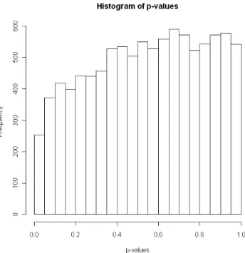
R> hist(chicken.raw$pval, main = "Histogram of p-values", xlab = "p-values") Figure 1 displays the histogram of the raw p-values, as produced by the command lines above. The shape of the histogram clearly shows an abnormal under-representation of the p-values in the neighborhood of 0. Indeed, if all the gene expressions were truly under the null hypothesis, the p-values should be uniformly distributed on [0,1] and the proportion of observed p-values under 0.05 should be close to 0.05, provided the gene expressions are independent. This marked departure of the empirical distribution ofp-values from the density function of a uniform distribution has been recently considered by some authors as the impact

Figure 1: Histogram of the rawp-values for the chickendataset.

of a high amount of dependence among tests (seeEfron 2007;Leek and Storey 2007;Friguet and Causeur 2010).

ThemodelFAMT function creates a R list with subclass FAMTmodel. This subclass is required for the main input of the other functions in the package. Thus, the summaryFAMT function can be applied to aFAMTmodelobject to get the list of positive tests for a control of the FDR at a preset level α (the default level is alpha = 0.15). Moreover, some useful information about the positive responses is provided, using the argumentinfo which gives the names of columns in theannotations component of chicken. Here, the columns namedID and Name give the gene identifier and the functional annotation of the significant genes.

R> summaryFAMT(chicken.raw, alpha = 0.05, info = c("ID", "Name")) $nbreject

alpha Raw analysis FA analysis

1 0.05 0 0

$DE

integer(0) $pi0

[1] 1

The nbreject component in the output of summaryFAMT is a table providing the number of positive tests using the raw multiple testing procedure and the factor analytic approach, for possibly different values of the FDR control levelα. In this special use of summaryFAMT

with nbf = 0, the columns named Raw analysis and FA analysis gives the same result since they are equivalent. The result shows no positive genes for a FDR control at level 0.05. The DE component of the output also provides the additional information on the responses specified in the argumentinfo.

Note that, if not explicitly provided as an input of the functionsummaryFAMTusing argument pi0, the proportionπ0 of true null hypotheses is estimated from the histogram ofp-values, by the method proposed byStorey and Tibshirani(2003), and returned in thepi0component of the output. Here, ˆπ0 = 1 is a direct consequence of the abnormal shape of the histogram of p-values as displayed in Figure1. Indeed, the dependence across genes induces a bias in the estimation ofπ0. Analysis of this dependence among gene expressions is addressed in section 5 but a first possible biological explanation is that all the chickens in this experiment are half sib males, which is to say genetically very similar.

This example is a typical situation where the dependence among genes must be taken into account to have a chance to reveal significant relationships between the hepatic transcriptome profile and the quantity of abdominal fatness.

4. Multiple testing dependence using FAMT

4.1. Method

The details of the method are described inFriguet et al. (2009). The main innovation with respect to most classical methods consists in capturing the components of dependence between variables into latent factors and integrating this latent structure in the calculation of the test statistics. It is indeed assumed that the conditional covariance matrix Σ of the responses, given the explanatory variables is represented by a factor analysis model:

Σ = Ψ+BB>, (2)

whereΨ is a diagonal m×m matrix of uniquenessesψ_k2 and B is a m×q matrix of factor loadings. In the above decomposition, the diagonal elements ψ_k2 inΨare also referred to as the specific variances of the responses. Therefore,B>Bappears as the shared variance in the common factor structure.

The factor analysis representation of the covariance is equivalent to the following mixed effects regression modeling of the data: fork= 1, . . . , m,

Y(k) = β(₀k)+x>β(k)+b>_kZ+ε(k), (3)

where bk is the kth row of B, Z = (Z(1), . . . , Z(q)) are latent factors supposed to

concen-trate in a small dimension space the common information in the m responses,Zis normally distributed with expectation 0 and variance Iq and ε = (ε(1), . . . , ε(m))> is a normally

dis-tributed m−vector, independent of Z, with mean 0 and variance-covariance Ψ. Therefore, factor analysis can be viewed as simultaneous mixed effects regression models sharing common covariance components.

An expectation-maximization (EM) algorithm inspired from Rubin and Thayer (1982) is used to estimate Ψ, B and Z (see Friguet et al. 2009 for details). Since this algorithm

only implies inversions of q ×q matrices, fitting the factor analysis (FA) model on high-dimensional datasets is computationally much less cumbersome than more usual algorithms such as Principal Factoring used in psychometrics. As recommended inFriguet et al.(2009), the number of factors is chosen according to anad-hocprocedure which consists in minimizing the variance of the number of false discoveries. Once the factor model is estimated, the so called factor-adjusted test statistics are derived asF-tests calculated on the adjusted response variablesY(k)−b>_kZ obtained by subtracting the dependence kernel from the data. Friguet

et al. (2009) show that the resulting test statistics are asymptotically uncorrelated, which improves the overall power of the multiple testing procedure.

4.2. Results of the FAMT analysis Optimal number of factors

The modelFAMT function implements the whole FAMT procedure with default options for the estimation ofπ0 and the number of factors. As mentioned in the previous section, the method proposed byStorey and Tibshirani(2003) is implemented to estimate π0.

Concerning the number of factors, the dependence in the residual correlation matrix resulting from the k-factor analysis model fitting induces an inflation of the variance of the number of false positives. This variance has a negative impact on the actual control of the false discovery proportion. Hence, as explained by Friguet et al. (2009), the number of factors considered in the model is chosen to reduce this variance. In order to avoid the overestimation of the number of factors, the function is implemented in such a way that the optimal number of factors corresponds to the largest number of factors for which the decrease of the variance inflation criterion is lower than 5 % of the previous value (see the Catell scree test criterion, Cattell 1966). Nevertheless, the optimal number of factors can also be specified by the nbf argument in themodelFAMTfunction (see the second illustrative example of this paper). Once the optimal number of factors is chosen, the model parameters are estimated using an EM algorithm. Factor-adjusted test statistics are derived, as well as the correspondingp-values. The testing issue is the same as in the previous section.

R> modelfinal <- modelFAMT(chicken, x = c(3, 6), test = 6) R> modelfinal$nbf

[1] 3

A side effect of themodelFAMT function is to produce a diagnostic plot, displaying the values of the variance inflation criterion along with the number of factors. Figure 2shows that the optimal number of factors obtained by themodelFAMT function, which is modelfinal$nbf = 3, also corresponds in this case to the minimum value of the variance inflation criterion. The model parameters are estimated with this choice of a 3-factor structure and π0 is estimated using the method byStorey and Tibshirani(2003) applied on the factor-adjusted p-values. The number of positive tests is provided for each level of FDR control chosen by the user (in our example below, the levels are defined by the argument alpha = seq(0, 0.3, 0.05)). The list of positive genes (DEcomponent) is given for the highest alpha.

Figure 2: Variance inflation criterion for the determination of the optimal number of factors.

$nbreject

alpha Raw analysis FA analysis

1 0.00 0 0 2 0.05 0 0 3 0.10 0 2 4 0.15 0 6 5 0.20 0 6 6 0.25 0 8 7 0.30 0 11 $DE ID 6722 RIGG05436 3885 RIGG04393 1119 RIGG15056 3484 RIGG05478 463 RIGG09893 124 RIGG12578 9859 RIGG03755 9840 RIGG04507 3925 RIGG10355 4968 RIGG05365 3855 RIGG13434

6722 Same gene X54200 3885 Weakly similar to CAE03429 (CAE03429) OSJNBa0032F06.12 protein

1119 ENSGALT00000015290.1

3484 ...ilar to Q8IUG4 (Q8IUG4) Rho GTPase activating protein (Fragment)

463 ENSGALT00000000452.1

124 ENSGALT00000008042.1

9859 Contig Hit 348847.1

9840 ...r to Q8AWZ8 (Q8AWZ8) Voltage-gated potassium channel subunit MiR 3925 Transforming protein p54/c-ets-1. [Source:SWISSPROT

4968 Genome Hit Contig7.437

3855 Troponin T fast skeletal muscle isoforms. [Source:SWISSPROT

$pi0

[1] 0.9738531

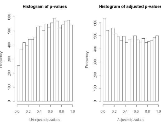
With a FDR control at level 0.15, there is no differentially expressed gene with the raw analysis, whereas 6 genes are differentially expressed with theFAMT analysis based on factor-adjusted tests statistics. In order to figure out the differences between both analyses, Figure3 compares the empirical distributions of the raw and the factor-adjustedp-values.

R> par(mfrow = c(1, 2))

R> hist(modelfinal$pval, main = "Histogram of p-values", + xlab = "Unadjusted p-values")

R> hist(modelfinal$adjpval, main = "Histogram of adjusted p-values", + xlab = "Adjusted p-values")

Factor-adjustment restores independence between test statistics, which results in a correction of the distribution of thep-values from the concave shape observed on the left panel plot of Figure 3. Indeed, it seems that a large amount of p-values are uniformly distributed and a few small p-values shall correspond to significant genes.

Note that the user can choose to focus on two aspects of the multiple testing procedure, which are the choice of the optimal number of factors with the nbfactors function and the estimation ofπ0 with thepi0FAMT function.

R> nbfactors(chicken, x = c(3, 6), test = 6, diagnostic.plot = TRUE)

This function gives the optimal number of factors as obtained from the modelFAMT function and produces the same plot as shown in Figure2.

The pi0FAMT function provides 2 algorithms to estimate π0. The density method is based onLangaas et al.(2005)’s approach where the density functionf of thep-value distribution is estimated assuming f is a convex function: the estimation of π0 is then f(p = 1). The smoother method uses the smoothing spline approach proposed by Storey and Tibshirani (2003). In most situations, these two methods give similar results but thesmoothermethod is numerically less time-consuming.

The following code uses thedensitymethod to estimateπ0 and produces a histogram of the p-values (Figure4), on which the convex estimation off is represented.

Figure 3: Histograms of raw p-values (left) and factor-adjustedp-values (right).

R> pi0FAMT(modelfinal, method = "density", diagnostic.plot = TRUE)

The estimated value of π0 is 0.95, which is slightly less than with the smoother method (ˆπ0 = 0.97).

5. Interpretation of the common factors

Thedefactofunction helps the user to give more insight on the common factors using some available external information on either response variables or individuals (see Blum et al.

2010). The external information is variables of covariates, which are not used in the model, and the categorical variables of annotations. As in principal component analysis (PCA), a transformation of the dataset allows to represent the individuals and variables graph through the matrix of factors loadings and the matrix of estimated factors. An analysis of variance test assesses the significance of the relationship between the factor and the external information. The use of this function requires aFAMTmodelas returned from the function modelFAMT and one or more explanatory variables incovariates. As the factors are designed to be indepen-dent from the explanatory variables (the abdominal fatness and the dam in our example), they shall be described according to the other covariates. In our example, the argument select.covar = 4:5 gives the 2 column numbers in covariatespicking two external vari-ables: Lotand Pds9s, which are respectively the hatch and the body weight of the chickens. Similarly, the argument select.annot = 3:6 picks 4 external variables in annotations: Block,Column,Rowand Length.

Figure 4: Estimation of the proportion of true null hypotheses using a non-parametric estimate of the density function of thep-values proposed byLangaas et al. (2005).

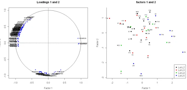
Figure 5: Loadings circle plot of the genes in thechicken example (left). Score plot of the microarrays in the chickenexample (right).

As for many implementations of PCA-like methods, two plots are provided to summarize the relationships between the latent factors extracted from the data and the external variables. First, if there are at least 2 common factors in the FA model, thedefactofunction provides a

loadings circle plot displaying the largest loadings along with two factors, the index of which are given by the argument axes (the default option is axes = c(1, 2)). Points are auto-matically labelled by their identifier as given in annotations (see Figure 5, left). Moreover, the score plot displays the coordinates of the individuals along the two factors, with different colors according to the levels of the factors selected incovariates(their hatch in thechicken example, see Figure5, right).

R> chicken.defacto <- defacto(modelfinal, axes = 1:2, select.covar = 4:5, + select.annot = 3:6, cex = 0.6)

In addition to these plots,F-tests are provided for the significance of the linear relationship between each component of the external information and each factor. The corresponding p-values are given in thecovariatesandannotations components of thedefactofunction. R> chicken.defacto$covariates Lot Pds9s Factor 1 0.006437319 0.27847793 Factor 2 0.258859549 0.00124608 Factor 3 0.271648846 0.96813322 R> chicken.defacto$annotations

Block Column Row

Loadings 1 8.148075e-25 0.2368072 0.21767892 Loadings 2 3.328477e-19 0.9323152 0.01889079 Loadings 3 0.000000e+00 0.1030426 0.68201616

The p-values inferior to a 5% treshold show a significant relation between the external infor-mation and the factor. Here, Factor 1 is clearly affected by a hatch effect, and Factor 2 by a body weight effect. Thus, part of the expression heterogeneity is probably due to these marked biological effects, which are independent of the abdominal fatness, the explanatory variable of the main interest in this study.

Moreover, some second-order technological biases turn out to have an impact on the corre-lation structure of the gene expressions, since the location of the spots on the microarray (Block, Column, and Row here) appears as significantly related to the loadings. According to Qiu et al. (2005), such kinds of effects on the correlation between gene expressions may be induced by the normalization procedure itself. The effect of Block is captured by all the factors, and the effect of Row by factor 2. The p-values of the effect of Column are all higher than the 5% treshold, so none of the factors are characterized by this effect.

6. Second illustrative example

The Animal Genetics Laboratory (INRA-Agrocampus Ouest, Rennes, France) studies the transcriptome profiling of the feeding-to-fasting transition in chicken liver. D´esert et al.

Figure 6: Variance inflation criterion along with the number of factors included in the model forD´esertet al. (2008) dataset.

Figure 7: Histograms of raw p-values and factor-adjusted p-values for D´esert et al. (2008) dataset.

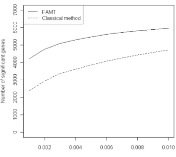
Figure 8: Number of significant genes with the raw method and FAMT forD´esertet al.(2008) dataset.

a global repression of cellular activity in response to this stressor. In this section, the related gene expression data are used to illustrate that the FAMT method is still useful to increase the power of the multiple testing procedure in a case where a large proportion of genes are significant.

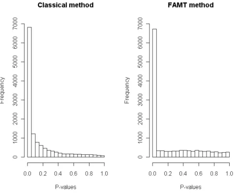
From the 20460 oligos present in the microarray data, 13057 aligning with a unique coding region of the 2.1 Washington University assembly of the chicken sequence genome, were cho-sen for statistical analyses. The dataset was finally restricted to 7419 genes (out of 13057) presenting a human ortholog with a human gene ontology (HUGO) symbol allowing for the recovery of functional annotations from these databases. 18 microarrays were analyzed: 6 corresponding to fed chickens, 5 to 16-hour fasted animals and 7 to 48-hour fasted animals. We calculate thep-values of the classical Fisher tests. The left panel plot of Figure 7shows that a large number of genes have smallp-values, which means that many genes are involved in the fasting process.

Figure6, resulting from themodelFAMTfunction, shows that the variance inflation criterion is minimum for 5 factors. Yet, themodelFAMTfunction proposesnbf = 1as optimal number of factors, using the Catell scree test criterion (see the previous section). In this case, the plot appears as a useful tool to modify, if necessary, the default number of factors resulting from modelFAMT. We finally chose to fit the factor analysis model with 5 factors.

The following code fits the FA model with 5 factors and extracts the numbers of rejected genes for the given FDR control levels.

R> model <- modelFAMT(Poulets, x = 2, nbf = 5)

R> plot(rejections[, 1], rejections[, 3], type = "l", lty = 1, + ylab = "Number of significant genes",

+ xlab = "False Discovery Rate control level", + ylim = c(0, 7000))

R> lines(rejections[, 1], rejections[, 2], type = "l", lty = 2) R> legend("topleft", c("FAMT", "Classical method"), lty = c(1, 2))

The number of significant genes for various FDR control levels are plotted in Figure8. For a same level of FDR control, more genes are considered as differentially expressed with the FAMT method than using the raw p-values. This illustrates that the FAMT procedure im-proves the power of the multiple testing procedure since, for a same FDR control level, more genes are significant.

7. Conclusion

The R package FAMT provides a powerful method for large-scale significance testing under dependence. It is essentially based on a factor modeling of the conditional covariance structure of the response variables. As these factors capture the dependence, they can be used to restore independence among tests, which results in a gain in terms of control of the false discovery proportion and on the overall power of the multiple testing procedure.

The main functions of the package are described in the paper, and are illustrated using a gene expression dataset available in the package. The package also offers tools to help the user describe and interpret the factors using some external information on either genes or arrays. The functions of the package, their arguments and values, are detailed in the help files. The websitehttp://famt.free.fr/ sums up theFAMTpackage and gives news about eventual updates.

Forthcoming versions of the package should include currently studied procedures aiming at inferring on the gene regulatory network using a Gaussian graphical model. Excel add-ins should also be included in the next update in order to help non-Rusers to analyse microarray data using FAMT.

References

Benjamini Y, Hochberg Y (1995). “Controlling the False Discovery Rate: A Practical and Powerful Approach to Multiple Testing.” Journal of the Royal Statistical Society B, 57, 289–300.

Black MA (2004). “A Note on the Adaptative Control of False Discovery Rates.”Journal of the Royal Statistical Society B,66, 297–304.

Blum Y, Le Mignon G, Lagarrigue S, Causeur D (2010). “A Factor Model to Analyze Het-erogeneity in Gene Expression.”BMC Bioinformatics,11(368).

Cattell RB (1966). “The Scree Test for the Number of Factors.” Multivariate Behavioral Research,1, 245–276.

Causeur D, Friguet C, Houee-Bigot M, Kloareg M (2010).Factor Analysis for Multiple Testing (FAMT): Simultaneous Tests under Dependence in High-Dimensional Data. R package version 2.20.0, URLhttp://CRAN.R-project.org/package=FAMT.

D´esert C, Duclos MJ, Blavy P, Lecerf F, Moreews F, Klopp C, Aubry M, Herault F, Le Roy P, Berri C, Douaire M, Diot C, Lagarrigue S (2008). “Transcriptome Profiling of the Feeding-to-Fasting Transition in Chicken Liver.”BMC Genomics,9(611).

Efron B (2007). “Correlation and Large-Scale Simultaneous Testing.”Journal of the American Statistical Association,102, 93–103.

Friguet C, Causeur D (2010). “Estimation of the Proportion of True Null Hypotheses in High-Dimensional Data under Dependence.”

Friguet C, Kloareg M, Causeur D (2009). “A Factor Model Approach to Multiple Testing under Dependence.”Journal of the American Statistical Association,104, 1406–1415. Hastie T, Tibshirani R, Narasimhan B, Chu G (2011). impute: Imputation for Microarray

Data. Rpackage version 1.26.0, URLhttp://CRAN.R-project.org/package=impute. Kim KI, Van de Wiel M (2008). “Effects of Dependence in High-Dimensional Multiple Testing

Problems.”BMC Bioinformatics,9(114).

Langaas M, Lindqvist BH, Ferkingstad E (2005). “Estimating the Proportion of True Null Hypotheses, with Application to DNA Microarray Data.” Journal of the Royal Statistical Society B,67, 555–572.

Le Mignon G, D´esert C, Pitel F, Leroux S, Demeure O, Guernec G, Abasht B, Douaire M, Le Roy P, Lagarrigue S (2009). “Using Transriptome Profiling To Characterize QTL Regions On Chicken Chromosome 5.”BMC Genomics,10(575).

Leek JT, Storey J (2007). “Capturing Heterogeneity in Gene Expression Studies by Surrogate Variable Analysis.”PLoS Genetics,3, e161.

Leek JT, Storey J (2008). “A General Framework for Multiple Testing Dependence.” Pro-ceedings of the National Academy of Sciences,105, 18718–18723.

Qiu X, Brooks A, Klebanov L, Yakovlev A (2005). “The Effects of Normalization on the Correlation Structure of Microarray Data.”BMC Bioinformatics,6(120).

RDevelopment Core Team (2011).R: A Language and Environment for Statistical Computing. RFoundation for Statistical Computing, Vienna, Austria. ISBN 3-900051-07-0, URLhttp: //www.R-project.org/.

Rubin DB, Thayer DT (1982). “EM Algorithms for ML Factor Analysis.”Psychometrika,47, 69–76.

Storey JD (2002). “A Direct Approach to False Discovery Rates.” Journal of the Royal Statistical Society B,64, 479–498.

Storey JD, Tibshirani R (2003). “Statistical Significance for Genomewide Studies.”Proceedings of the National Academy of Sciences,100, 9440–9445.

Affiliation: David Causeur Agrocampus Ouest

Applied Mathematics Department 65 rue de St-Brieuc

35000 Rennes, France

E-mail: [email protected]

URL:http://www.agrocampus-ouest.fr/math/causeur/

Journal of Statistical Software

Volume 40, Issue 14 Submitted: 2010-07-09