Statistical Analysis of Transposon Sequencing Data to Determine Essential Genes

(1)

STATISTICAL ANALYSIS OF TRANSPOSON SEQUENCING DATA

TO DETERMINE ESSENTIAL GENES

A Dissertation by

MICHAEL A. DE JESUS ANEIRO

Submitted to the Office of Graduate and Professional Studies of Texas A&M University

in partial fulfillment of the requirement for the degree of DOCTOR OF PHILOSOPHY

Chair of Committee, Thomas R. Ioerger Committee Members, Tiffani L. Williams

James C. Sacchettini Ricardo Gutierrez-Osuna Head of Department, Dilma Da Silva

December 2016

Major Subject: Computer Science

(2)

ABSTRACT

Transposon Sequencing (TnSeq) has become a popular biological tool for assessing the phenotypes of large libraries of bacterial mutants at the same time. This allows for high-throughput identification of genes which are essential for growth, thus providing valuable information about the function of those genes and the discovery of potential drug targets that could lead to treatments.

However, analysis of data obtained from TnSeq is challenging as it requires estimat-ing unknown parameters from data that is often noisy and likely comestimat-ing from a mixture of different phenotypes. In addition, the classification of essentiality is not known a priori, re-quiring unsupervised methods capable of identifying key features in the data to confidently determine essentiality.

We present several models capable of identifying essential genes while overcoming the difficulties that are present in analyzing TnSeq data. Together, these methods provide ways to analyze TnSeq data in one or multiple conditions, confined within gene boundaries or across the entire genome, and while reducing the impact of noise and outliers that are often present in this type of data.

(3)

(4)

ACKNOWLEDGMENTS

I would first like to thank my advisor, Dr. Thomas Ioerger, for his assistance and insight through out my studies. His impressive knowledge and infectious work ethic have been invaluable in this entire process. I would also like to thank my committee members, Dr. James C. Sacchettini, Dr. Ricardo Gutierrez-Osuna, and Dr. Tiffani L. Williams, for their guidance and input.

I would like to thank our collaborators Jason Zhang, Jennifer Griffin, Subhalaxmi Nambi, Richard Baker, Clare Smith, Andrew Olive, and Christopher Sassetti for their help and cooperation in this research.

Finally, I would like to thank my family for their support, and &TOTSE for making me the weird kid I am today.

(5)

LIST OF FIGURES

FIGURE Page

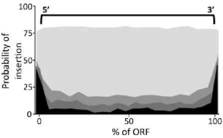
1.1 Example diagram of transposon mutagenesis . . . 3 1.2 Diagram of the TraSH method. Source: Sassetti (2003) [11] . . . 4 1.3 Frequency of insertions as percentage of the ORF. Darker shades

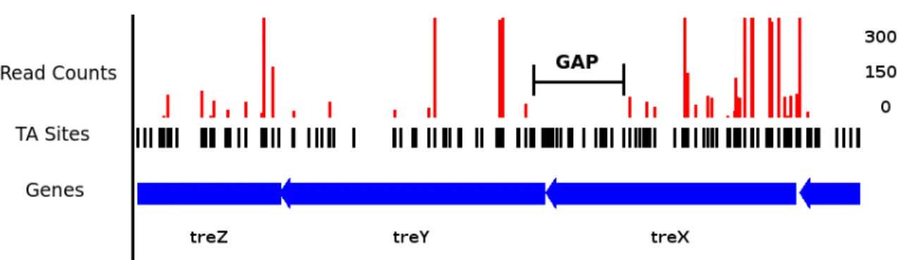
rep-resent genes with higher probability of being essential. Essential genes have a high likelihood of observing insertions near the 5’ and 3’ ends, and a non-zero probability of containing insertions across the entire coding-region. Source: Griffin et al. (2011) [17] . . . 7 2.1 Insertion pattern for TreX, a gene involved in trehalose biosynthesis.

The presence of a long gap a region of sites without any insertions -suggests the gene may code for a protein domain that plays an essential role. . . 12 2.2 Gumbel distributions with different values ofϕ andn. . . . 14 2.3 Plot of sortedZ¯ivalues for all genes. The averageZiof the final

sam-ple for all genes was estimated, and plotted in ascending order. The dashed lines represent the respective thresholds for the two categories of essentiality: Z¯i>0.9902andZ¯i<0.0371 . . . 26 2.4 Example genes with essential domains. Essential domains are

indi-cated in red, and non-essential domains (as predicted by PFAM) are indicated in yellow. . . 27 3.1 Histogram of the number of insertions within windows of 20 TA sites

(gray bars). A beta-binomial model with a variable insertion frequency is capable of fitting the observed data (black line). . . 32 3.2 Kernel density estimates for the mean posterior insertion probability

(black-solid) and observed insertion frequency (gray-dashed) for all the genes. . . 39 3.3 Kernel density estimates for the posterior insertion probability of

DnaA (Rv0001), a known essential gene involved in DNA repair, and MmpL11 (Rv0202c), a known non-essential gene believed to function as a transmembrane protein. . . 40

(9)

3.4 Insertion density for PPE5 (solid), PPE19 (dashed) and RpmB (dot-dash). All three genes contained an observed insertion frequency of 0.7, although they had different sizes (# TA sites). The insertion den-sity of the genes reflects the uncertainty that exists in smaller genes as these contain a smaller number of TA sites (Bernoulli trials). . . 44 4.1 (A) Diagram of the fully-connected HMM structure. From left to right,

the states represent read counts of increasing magnitude (essential, growth-defects, non-essential, and growth-advantage). (B) Diagram of the states for a local sequence of ∼20 TA sites, with state labels (underneath), transitions (from qi−5 to qi+13 ) and their

correspond-ing emissions (i.e. read counts). A transition is shown from the non-essential state to the non-essential state at time i, as the essential state is most likely to explain the consecutive observations of no insertions (fromqitoqi+13) . . . 49

4.2 Histogram of read-counts for a library ofM. tuberculosistransposon mutants (black, solid vertical lines), fitted with a geometric distribu-tion with parameterθ =1/c¯(dashed line). . . 51 4.3 Log-log plot of geometric likelihood functions for the essential,

growth-defect, non-essential and growth-advantage states. . . 53 4.4 Read counts and state classifications for a∼57 kb region of the H37Rv

genome is shown. Essential regions are shown in green, growth-defect regions in yellow, non-essential regions in red, and growth-advantage regions in blue. Read counts are truncated at 2,000 (with a max of

∼3,000 in this region), and the mean read count in the library is rep-resented by a gray horizontal line. . . 55 5.1 Top 100 reads from a M. tuberculosis TnSeq dataset. A large

read-count with a magnitude >200,000 is present in this dataset. This single site has a large impact on the mean read-count. . . 69 5.2 Top 100 reads from a M. tuberculosis TnSeq dataset. A large

read-count with a magnitude >200,000 is present in this dataset. This single site has a large impact on the mean read-count. . . 70 5.3 Histogram of the difference in means generated by permuting counts

(including zeros)before normalization. The red-line represents the observed difference in means before normalization (-101.62) . . . 73

(10)

5.4 Histogram of the difference in means generated by permuting counts (including zeros) after normalization by TTR. The red-line repre-sents the observed difference in means before normalization (-101.62) 75 5.5 (a) Histogram of non-zero read counts obtained fromM. tuberculosis

tn-mutant libraries. A1, A2 are replicates grown in vitro, and B1 and B2 are replicates grown in vivo. The black line represents a Geometric fit. (b) Histogram of read counts on a log scale. . . 77 5.6 QQ-plot of the raw read counts for dataset B2, and the theoretical

Ge-ometric quantiles. . . 78 5.7 (a) Example of a Beta distribution with ρ =0.05, and κ = 40. (b)

Histogram of counts from a regular Geometric distribution (p=0.05, black curve), and a Beta-Geometric distribution (ρ =0.05, κ =40, red). . . 80 5.8 Resampling histogram for theM. tuberculosisgene Rv0017c, grown

in vitro and in vivo. Rv0017c has 23 TA sites, and the sum of the observed counts at the TA sites in this genesin vitrowas 1,318 andin vivowas 399, therefore the observed difference in counts is -918. To determine the significance of this difference, 10,000 permutations of the counts at the TA sites among the datasets was generated and the observed differences plotted as a histogram showing that a difference as extreme as -918 almost never occurs by chance. The p-value is determined by the tail of this distribution to be 0.003 (30 out of 10,000). 82 5.9 Histogram of log-fold change in mean read-count per gene after

nor-malizing read-counts in the presence of outliers. NZMean (a) and To-tal Reads (b) are susceptible in the presence of outliers. On the other hand, TTR (b) and BGC (d) are robust to outliers, as the peak of the distribution is centered around zero as expected in replicate datasets. . 85 6.1 Visual representation of the multiplicative model of genetic

interac-tions. If the double mutant (∆X×∆Y) incurs a greater reduction in fit-ness than expected, then this suggests a negative interaction between gene X and gene Y. If the double mutant exhibits better fitness, then this suggests there is a positive interaction between them. . . 87 6.2 Depiction of genetic interactions in TnSeq data . . . 89 6.3 (A) Possible comparisons of different datasets available in this

exper-imental setup. (B) Illustration of change in mean-read count across time-points between the strains. . . 91

(11)

6.4 Visual description of how the method works. Read picture from bot-tom up. (1) Distributions of the mean read-counts are generated for the 4 conditions: WT-0, WT-32, KO-0, and KO-32. (2) We calculate the logFC between the samples for each strain, to get two distribution of logFC. (3) We take the difference of the two logFC distributions to get a single distribution of the difference between logFC of the strains. (4) We compare the overlap of the distribution of the differences with the null hypothesis of no difference to assess significance. . . 94 6.5 Plot of the mean read-counts (log-scale) for Rv1431 (panel A) and

DrrA (panel B) between H37Rv (WT) and the knockout strain of Rv1432 (KO). Rv1431 illustrates a suppressive interaction with Rv1432, while DrrA shows an aggravating interaction. . . 97 6.6 Genetic interactions with Rv2680. Genes on the left showed positive

interactions, while genes on the right showed negative interactions. The genes are colored by functional category: Yellow: intermediary metabolism and respiration, Orange: lipid metabolism, Red: cell wall and cell processes, Blue: PE/PPE, Purple: insertion seqs and phages, Green: virulence, detoxification, adaptation, Light Grey: conserved hypotheticals, Dark Grey: regulatory proteins, White: Unknown. . . 99

(12)

LIST OF TABLES

TABLE Page

2.1 Statistics for essentials, non-essentials and uncertain genes. Non-essential genes are those withZi<0.05, Essential genes are those with Zi>0.95. Average span is in nucleotides. . . 25 2.2 Comparison of essentiality predictions with TraSH analysis. The

re-sults obtained by Sassetti. et. al are compare with those obtained with our Gumbel method for genes in M. tuberculosis. Genes for which the TraSH method did not produce data, are labeled ”no-data”. Genes with less than four TA sites were labeled ”Short” as they could not be analyzed by the Gumbel method. . . 28 3.1 Essentiality comparison between the TraSH method and the

Local-Frequency Model. . . 42 3.2 Essentiality comparison between the Global Frequency Model (GFM)

and the Local Frequency Model . . . 43 5.1 False positives (p_adj.<0.05) obtained by each normalization method,

after running on replicates of the libraries. . . 84 6.1 Types of genetic interactions identified for the three knockout (KO)

strains analyzed. Negative interactions result in reduced fitness for the double mutant (Aggravating). Positive interactions improve fit-ness relative to the expected fitfit-ness deficit of the double mutant (Al-leviating), or completely suppress any negative effects of the double mutation (Suppressing). . . 96

(13)

1 INTRODUCTION

1.1 Motivation

Identifying genes that are essential for growth of bacterial organisms is important for the development of drugs that inhibit the function of a crucial protein, thus possibly be-coming a target for treatment of infectious bacteria. For instance isoniazid and rifampicin, which are first-line drugs used to treat tuberculosis, both bind to proteins that play essential roles (InhA and DNA Polymerase respectively) thus preventing the growth of the pathogen [1, 2]. Furthermore, if the essentiality of a gene is shown to depend on a particular con-dition, this can provide valuable insight on the function of unknown proteins. In order to identify which genes are essential, individual bacilli are mutated in such a way that the function of one (or more) of its genes is interrupted. This can be done in a high-throughput fashion by using a small fragment of DNA (called a transposon) to disrupt random locations in the genome, thus allowing for the creation of large libraries of mutants. However, bot-tlenecks in previous sequencing methods did not allow for the sequencing of large libraries of mutants at the same time. New advances in sequencing have made it possible to rapidly sequence an entire library of thousands of such mutants simultaneously. By sequencing large libraries of transposon mutants, researchers have access to high-resolution sequence data that reveals which specific areas of the genome can be disrupted by a transposon, providing valuable information about their need for an organism’s viability.

(14)

of new information about essentiality, there are a large number of issues that make any analysis of this data challenging. As mutant libraries represent those bacteria that survived a transposon insertion in their DNA, the resulting data reflects only those regions which are capable of tolerating disruption. However, genomic regions lacking any insertions do not necessarily imply that the area is essential to the organism. These areas may represent sites that were simply missed by chance (as not all potential insertion sites are saturated when construction a transposon library) but are otherwise non-essential to the organism (and thus would have tolerated insertion of a transposon if one had occurred there). In this sense, TnSeq data can be thought of as a missing data problem where the disruptability of empty sites is unknown and most be determined statistically. Furthermore, as the essen-tiality of genes is not known beforehand, unsupervised methods are required to confidently determine which genes are necessary. While transposon insertions are supposed to disrupt the function of the genomic regions where they insert, in reality essential genes are often able to tolerate some insertions. For instance, it is common to observe insertions in the N-and C-terminus of a gene as the protein may still able to be translated N-and fulfill its biolog-ical function despite the insertion [3, 4, 5]. Thus, although initially one may be tempted to determine essentiality based on whether a gene has evidence of insertions or not, more sophisticated statistical models are required.

(15)

1.2 Background

1.2.1 Transposon Mutagenesis

In order to determine essentiality it useful to observe how an organism copes with the loss of a gene’s function. A popular technique used to disrupt the function of a genomic re-gion is transposon mutagenesis. In transposon mutagenesis, a mutation is mediated through the insertion of a transposon at a random position in the genome. Transposons are small fragments of DNA (typically 1-2kb long) that can insert within the chromosomes of an organism [6]. Different transposons exist with varying characteristics like local-sequence preference [7, 8, 9]. The Himar1 transposon, for example, has shown specificity for ar-bitrary TA dinucleotides [8]. As the entire DNA sequence of a bacterial organism can be known beforehand through sequencing, the preference for TA dinucleotides can be used to know which sites may be targeted by the transposon.

Figure 1.1: Example diagram of transposon mutagenesis

Using transposon mutagenesis, large libraries of mutants are constructed with dis-ruptions at random locations of the genome. The resulting libraries are grown under en-vironmental conditions of interest, thus potentially revealing phenotypes for the mutants.

(16)

Determining what disruption resulted in the phenotype observed, however, requires iden-tifying the location of the transposon insertion.

1.2.2 Transposon Site-Hybridization (TraSH)

Transposon Site-Hybridization (TraSH) was a previous attempt to determine essen-tiality using transposon mutant libraries. In order to identify the location of insertions, TraSH used micro-array hybridization to figure out what genes in the mutant libraries where being expressed and which ones where not [10]. Primer extension was used to amplify from the regions at the ends of the transposon out into the surrounding genomic regions, and these products where then identified by hybridization to gene-specific probes (Figure 1.2). Thus, genes which are non-essential for growth are those which hybridize to the probes in rates similar to the background rate. Those genes which are essential for growth, and thus do not have surviving mutants in the library, would represent those which hybridize as significantly lower rates. Using this approach, genes essential for growth in variety of organisms likeM. tuberculosisandB. anthraciswere identified [11, 12, 13].

(17)

Although one can obtain a general a idea of what genes were being expressed through the use of TraSH, it does not provide high-resolution information about where the insertions took place. In addition, a serious statistical treatment of the data produced by TraSH is made difficult by the fact that the assessment of essentiality is limited to measurements of hybridization at a few probes (i.e. 4) for each gene. With the advent of new sequencing technology, it become possible to determine the exact location of insertions, thus replacing the need for TraSH.

1.2.3 Transposon Sequencing (TnSeq)

With the development of high-throughput sequencing, large libraries of mutants can be sequenced at the same time, providing the exact location of the transposon insertions. This technique, called transposon sequencing (TnSeq), helps overcome many of the limi-tations of previous methods. Once libraries of transposon mutants are created and exposed to the desired conditions, the surviving mutants are sequenced using deep-sequencing. The resulting sequence reads are mapped to the genome to determine the precise coordinate of the transposon insertions. While the number of reads mapping to any given location should be proportional to the number of mutants in the library, the number of reads can be affected by artifacts like PCR amplification. More modern protocols utilize barcodes to ensure that counts at a position represent unique insertions [14].

TnSeq has been successfully used to analyze essentiality in a number of different organisms and growth conditions [15, 16, 17]. However, despite being used since 2009, there was a lack of rigorous statistical methods capable of analyzing the large amount of

(18)

data produced by TnSeq. Initial attempts to determine essentiality through TnSeq tended to rely on arbitrary thresholds of fitness, or ad-hoc criteria to overcome the difficulties of analyzing this data. For instance, since essential genes are often capable of sustaining insertions at the N- and C- termini, these methods often required the exclusion of the first and last 5-20% of a gene’s coding region so as to not label these genes as non-essential [15].

1.3 Related Work

One of the earliest approaches to analyzing TnSeq data was work done by Natalie Blades and Karl W. Broman [18]. Their method utilizes a multinomial function to char-acterize the number of mutants with transposon insertions unique to a gene, as well as the number of mutants with transposon insertions that occur in coding regions that are shared (overlap) between two adjacent genes. This last feature is meant to capture the uncertainty that exists when the coding regions of adjacent genes overlap, and thus a transposon inser-tion cannot be definitively assigned to one particular gene. One important limitainser-tion of the approach used by Blades and Broman, is that it assumes that any gene with a transposon in-sertion is considered to be non-essential. Thus, they focused on estimating the probability of a gene being essential given that it was devoid of insertions, the number of sites within the gene, and the overall saturation of the library. This assumption is useful in the case of libraries with very low saturation (i.e. libraries with few mutants and little sequence data available) as was common before the advancement in sequencing technology. However,

(19)

Figure 1.3: Frequency of insertions as percentage of the ORF. Darker shades represent genes with higher probability of being essential. Essential genes have a high likelihood of observing insertions near the 5’ and 3’ ends, and a non-zero probability of containing insertions across the entire coding-region. Source: Griffin et al. (2011) [17]

it is not true that a gene with a transposon insertion must be non-essential. Most genes, including essential genes, have a high probability of tolerating insertions within the 5’ and 3’ terminal ends (N- and C- termini) of the gene, but may tolerate insertions in other parts of the gene as well (Figure 1.3).

To address the insertability observed at the terminal ends of genes, methods would often ignore insertions that occurred within a predetermined distance of the termini. For instance Gawronski et al. [15] excluded insertions that occurred in the first 5% and last 20% of a gene’s coding region. Criteria like this require assuming a certain fixed cut-off distance at which the transposon insertions would disrupt a genes functions when they occur in the ends. However, this is unlikely to be equal for all proteins. More importantly, essential genes can allow insertions at other areas of the gene, if they contain non-essential

(20)

protein domains or at linkers within genes [19].

Other methods for analyzing TnSeq data have borrowed from the RNA-Seq litera-ture. Like TnSeq, RNA-Seq is based on counts of reads obtained from sequencing [20]; thus much of the same methodology can be used for both types of data. A popular choice for analyzing RNA-Seq data is edgeR [21], which utilizes a Negative Binomial distribution to assess the likelihood of the read-counts observed within a gene. One of the advantages of the Negative Binomial model is that it can represent over-dispersion in the data that is typ-ically observed in biological datasets. It can also be extended to account for the abundance of sites with no insertions (i.e. counts of zero), by using a zero-inflated Negative Binomial model. Given the success of the Negative Binomial model in analyzing RNA-Seq data, Zomer et al. [22] developed software called ESSENTIALS which utilizes edgeR as the underlying analysis method to distinguish between essential and non-essential genes.

Unfortunately, ESSENTIALS is also hindered by the presence of insertions at the terminal ends or non-essential domains of essential genes. As edgeR takes the total number of read-counts that occur within a gene, any essential gene which tolerates some insertions will tend to have a higher number of read-counts compared to essential genes that are completely devoid of insertions. Thus, ESSENTIALS tends to underestimate the number of essential genes, classifying genes that can tolerate some insertions, as non-essential.

Most of the methods mentioned so far limited to determining essentiality within pre-defined genetic boundaries like the coding-region of a gene. However, the essentiality of regions outside of genes is also important, as these may include genomic features that

(21)

play important roles (e.g. like binding sites for transcription factors or DNA methylation sites). Methods meant to analyze the essentiality of an entire genome often depend on a sliding-window approach, where the read-counts that occur within an specified window of insertions sites (or nucleotides) are compared to some null distribution [23, 24].

Aside from not being limited to coding-regions, another advantage of these ap-proaches is that they are not susceptible to insertions at the terminal ends of ORFs or within domains. However, sliding-window approaches require predetermined choice for length of the sliding-window, which can significantly impact how much influence is exerted by neighboring insertions sites. A more rigorous methodology would be preferable in these cases, as it is often not obvious which window-size would be best (or more justified) for determining essentiality.

1.4 Scope and Contribution

In this dissertation, several statistical models for determining essentiality from TnSeq data are presented. Each method discussed here represents a novel approach to overcoming the difficulties of analyzing TnSeq data, and led to a publication that outlined the method-ology:

• Section 2 presents a Bayesian model of essentiality that identifies the unusually long stretches of sites without insertions that are typical of essential genes (or domains) [17, 25]. In doing so, it overcomes the difficulties that exist in identifying genes that can tolerate insertions at their terminal ends or contain non-essential domains.

(22)

• Section 3 presents a hierarchical Bayesian model of essentiality that estimates indi-vidual insertion probabilities for each gene, thus relaxing assumptions made by most other models (which typically assume genes share a single parameter representing insertion probability or mean read-count) [26, 27].

• Section 4 presents a Hidden Markov Model (HMM) to determine the essentiality of an entire genome [28]. This HMM set itself apart from most other methods since it has four states representing four different categories of essentiality (or levels of fitness).

• Section 5 describes how to identify conditionally essential genes (genes that are es-sential in one condition but not another), and presents two different methods that nor-malize datasets with different saturation levels, number of reads, and skew [29, 30]. • Section 6 presents a novel method capable of identifying genetic interactions by com-paring TnSeq datasets of different strains grown under two experimental conditions. These (and other) methods are provided in a graphical software package called TRANSIT [31].

(23)

2 DETERMINING ESSENTIAL GENES BY DETECTING

UNUSUALLY LONG GAPS

*

2.1 Introduction

The primary goal of analyzing transposon mutagenesis datasets is to determine which genes are essential for growth under a specific condition. As transposon insertions disrupt the function of the genomic regions they insert in, those that occur in essential genes will render the organism unable to carry out necessary functions for survival.

The underlying idea behind the Gumbel Model of essentiality is that genes that are essential will have unusually long stretches of the genome without any observable transpo-son insertions [17, 25]. These regions would appear as “gaps” in the transpotranspo-son insertion pattern (Figure 2.1), and would indicative of the essentiality of a region as they are unlikely to occur by chance. On the other hand, because the organism is capable of tolerating in-sertions in non-essential regions, those areas should exhibit gaps that are as long as would be expected given the saturation of the library.

Because the Himar1 transposon inserts specifically at TA dinicleotides, the number of TA sites in a given gene (and which of them had an insertion) can be easily determined from the data. In an analogy to a sequence of coin tosses, each TA site can be viewed as an independent Bernoulli trial with a parameter representing the probability of success. *_{DeJesus, M.A., Zhang, Y.J., Sassettti, C.M., Rubin, E.J., Sacchettini, J.C., and Ioerger, T.R., “Bayesian} analysis of gene essentiality based on sequencing of transposon insertion libraries”, Bioinformatics, 2013, 29(6), 695-703, by permission of Oxford University Press.

(24)

Figure 2.1: Insertion pattern for TreX, a gene involved in trehalose biosynthesis. The presence of a long gap - a region of sites without any insertions - suggests the gene may code for a protein domain that plays an essential role.

A sequence of TA sites in a row without any transposon insertions (or “run”) is therefore analogous to a sequence of heads in a row. The expected value and the variance of the largest run of heads in a row are given by the following equations [32]:

ERn=log1/ϕ(n(1−ϕ)) +γ/ln(1/ϕ)−1/2+r1(n) +ε1(n) (2.1)

VarRn=π2/6ln2(1/ϕ) +1/12+r2(n) +ε2(n) (2.2)

where n represents the number of coin tosses (or sites), ϕ represents the probability of heads (or probability of non-insertion), andr1,r2,ε1, andε2are small correction terms.

To model the distribution of the largest run in a series of trials, the Extreme Value distribution (or Gumbel distribution) is utilized. The Gumbel distribution is part of the exponential family of distributions, and has the following form:

Gumbel(x;µ,σ):= 1 σe−z−e −z z=x−µ σ (2.3)

(25)

with location and scale parametersµ andσ respectively. The Gumbel distribution models the distribution of extreme or maximum values obtained from a finite set of independent and identically distributed samples. By maximizing over repeated samples of values, the shape of the Gumbel distribution is skewed to the right, producing a “fatter” tail in the right side of the distribution, allowing for extreme values to have a higher probability than being observed than they normally would with the underlying distribution.

Combining Equations 2.1 and 2.2 with the formulas for the mean, and variance of the Gumbel distribution (ignoring the negligible correction terms for simplicity) results in the following parameters:

µ =log1

ϕ(n(1−ϕ)) (2.4)

σ = 1

ln_ϕ1 (2.5)

wherenis the number of trials (or TA sites) and ϕ is the probability of observing a head (or empty TA site).

Figure 2.2 shows distributions of the longest runs of heads in a series of coin tosses for different values ofnand different values ofϕ. The expected maximum run scales up logarithmically innand1−ϕ asn.

followingcreditlineappearswhereverthematerialisused:author, ti-tle,journal,year,volume,issuenumber,pagination,bypermissionofOxford University-Pressorthesponsoringsocietyifthejournalisasocietyjour

(26)

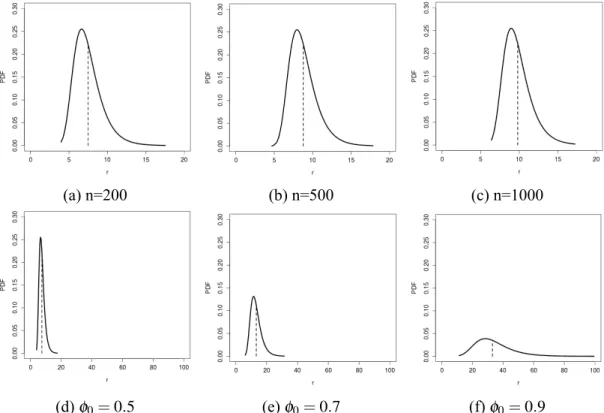
(a) n=200 (b) n=500 (c) n=1000

(d)ϕ0=0.5 (e)ϕ0=0.7 (f)ϕ0=0.9 Figure 2.2: Gumbel distributions with different values ofϕ andn.

The first row of figures shows how the distribution behaves while varying the number of trials,n, and using a fixed probability of successϕ =0.5. The second row shows how the

distribution behaves while varying the probability of success,ϕ,in a fixed number of trials,n=200. The vertical dashed lines shows the expected maximum run according to

(27)

non-insertion,ϕ, is unknown. This parameter is crucial to estimate in order to determine the probability of a gene being essential. Section 2.2 formally describes the Bayesian model of the data while Section 2.3 describes the posterior distributions and how the variables are estimated.

2.2 Data Model

LetYi={ri,si,ni} represent our observations for thei-th gene for i=1...G, where nirepresents the total number of TA sites,rirepresents the number of TA sites spanned by the largest run of non-insertions, and sirepresents the number of nucleotides spanned by the largest run. The essentiality assignments for all genes is represented by the unknown variableZ, with the individual assignment fori-th gene represented by the boolean vector Ziwhich accepts binary values of 0 and 1 for non-essential and essential genes respectively. These two classes of genes represent the two categories found in the mixture model. The mixture coefficient representing the prevalence of the category in the mixture is given by ω = {ω1,ω0}. Finally, we assume a global non-insertion probability, ϕ0, that governs

probability of non-insertions across all non-essential genes. This is 1 minus the insertion density observed at non-essential genes.

We wish to estimate a complete joint probability density,p(Z,Y,ϕ0), which combines

the observed data as well as the unobserved parameters of the model. Using Bayes theorem we can use the joint distribution to derive conditional distributions from which we can obtain estimates of the essentiality for the genes conditional on the data p(Z|Y,ϕ0). To

(28)

accomplish this we rewrite this joint probability in terms of the likelihood of the data and our prior expectations:

(Y|Z,ϕ₀)∗p(Z)∗p(ϕ₀) (2.6)

Since we assume independence among genes the likelihood can be written as a prod-uct of the individual observations:

p(Y|Z,ϕ0∝

∏

i p(Yi|Z,ϕ0) (2.7) =

∏

i p(si,ri,ni|Zi,ϕ0) (2.8)

Due to the definition of the joint probability, the joint likelihood of the data (i.e. p(si,ri,ni)) may be specified different ways (i.e.P(A,B) =P(A|B)P(B) =P(B|A)P(A):

p(Yi|Z,ϕ0) =p(ri,ni,si|Z=0,ϕ0)

=p(ri,ni|Z=0,ϕ₀)×p(si|ri,Z=0,ϕ₀) =p(si|Z=1,ϕ0)×p(ri,ni|si,Z=1,ϕ0)

This fact is useful different distributions can be used to represent the mixture of essential and non-essential genes. Sections 2.2.1 and 2.2.2 show the specification of the likelihoods for non-essential and essential genes respectively.

(29)

2.2.1 Likelihood for Non-Essential Genes

As non-essential genes are not required by the organism, they are expected to with-stand disruption at levels that correspond to the probability of insertion in the library (i.e. the saturation of the library). The length of the maximum run of insertions in a non-essential gene should therefore conform to the Gumbel distribution, given the non-insertion proba-bilityϕ0: p(ri|Zi=0,ϕ0,ω1) =Gumbel(x;m,τ) = 1 τe−z−e −z (2.9)

wheremandτ represent location and scale parameters.

Sinceri andsiare highly correlated, we model their dependence as linear-Gaussian distribution, with covariance matrix Σ=[[σ_r2,σr,s],[σr,s,σ_s2]] estimated a priori from empirical data:

p(si|ri,Z=0,ϕ0,ω1)∼N(si−λrri,σr2) (2.10) were λr and σr are the parameters of the Normal distribution, derived from the Linear Gaussian relationship (i.e. λr =σr,s

σr ) observed in the data.

The likelihood for a non-essential gene is therefore: p(Yi|Z,ϕ0) =p(ri,ni,si|Z=0,ϕ0) =p(ri,ni|Z=0,ϕ0)×p(si|ri,Z=0,ϕ0) =Gumbel(x;m,τ) = 1 τe−z−e −z × ∼N(si−λrri,σr2)

(30)

2.2.2 Likelihood for Essential Genes

Unlike non-essential genes, those genes which are necessary for the growth of the organism will have stretches of TA sites lacking insertions that are longer than would we expected by chance. This requires using different distributions to describe the likelihood.

p(ri,si|Zi=1,ϕ0,ω1) =

p(si|Z=1,ϕ0,ω1)×p(ri|si,Z=1,ϕ0,ω1)

We model the likelihood of observing a span of nucleotides (si) with a normalized sigmoid (logistic) function that is relatively uniform as long as the gene contains a gap that is as large as a typical protein domain. Using this likelihood allows our method to disambiguate those cases where the run of non-insertions actually represents a smaller or larger segment of the genome than suggested by the number of consecutive TA sites without insertions:

p(si|Zi=1) =Ω(si;δ) = C

1+e0.01∗(δ−x) (2.11) whereδ is the mean number of nucleotides spanned by an average protein domain, andC is a normalization constant. Previous studies of the length of domains within proteins have found the average size to be roughly 100 amino-acids or 300bp [33]. Using this threshold forδ, the likelihood of observing a given spansiis more or less uniform, except it is near 0 if the the longest run of non-insertions spans less than about 300bp.

(31)

As with non-essential genes, the likelihood of observing a span of nucleotides ri givensiis modeled through a linear-Gaussian dependence similar to Equation (2.10), but with an inverse relationship (i.e. N(ri−λssi,σs2)). The joint likelihood of the observations at essential genes is therefore:

p(ri,si|Zi=1,ϕ0,ω1) =Ω(si)×N(ri−λssi,σs2) (2.12)

2.3 Parameter Estimation

To estimate the parameters of interest, including the probability of essentiality, the posterior distributions of these unknown parameters must first be derived. A prior distri-bution for these parameters is also required.

2.3.1 Posterior Distribution ofω

The prior distribution of the mixture coefficient,ω, can be taken to be a Beta distribu-tion. The Beta distribution is a common choice for a prior on a probability parameter as its support is defined in the interval [0,1] and it is conjugate with other common distributions. The posterior distribution is derived as follows:

p(ω1|Y,Z,ϕ0)∝π(Z|ω1)×π(ω1)

∝Binomial(Kz1;ω1,G)×Beta(ω1;αw,βw)

∝Beta(ω1;αw+Kz1,βw+G−Kz1)

(32)

2.3.2 Posterior Distribution of Z

The probability of essentiality is estimated through the indicator variable,Zi, which indicates which mixture (or essentiality class) the gene belongs to. As there are two pos-sible essentiality classes, the posterior is given for both pospos-sible values (i.e., Zi =1 and Zi=0): p(Zi=1|Y,Z_{−i},ϕ0,ω1) ∝p(si|Zi=1)×p(ri|si,Zi=1)×π(Zi=1|ω1) ∝ Ω(si)×N(ri−λssi,σs2)×ω Zi=1 1 (1−ω1) 1−Zi=1 (2.14) p(Zi=0|Y,Z_{−i},ϕ0) ∝p(ri|Zi=0,ϕ0)×p(si|ri,Zi=0)×π(Zi=0 |ω1) ∝Gumbel(ri|m,τ)×N(si−λrri)×ω₁Zi=0(1−ω1)1−Zi=0 (2.15)

As there are only two possible values, the posterior probability of an individualZi therefore a Bernoulli distribution:

Zi=Bernoulli( p1 p1+p0 ) p1=p(ri,si|Z{−i},ϕ0)×ω1 p0=p(ri,si|Z_{−i},ϕ0)×(1−ω1)

(33)

2.3.3 Posterior Distribution ofϕ0

As a prior for the non-insertion probability,ϕ0, the Beta distribution is chosen. As

the likelihood of non-essential genes is the only one which depends onϕ0, others can be

discarded as constants with respect to ϕ0. Unfortunately, the remaining likelihood is a

product of Gumbel distributions (for individual non-essential genes). This likelihood is not conjugate with any known distribution, thus the resulting posterior distribution does not have standard form that is easy to sample from:

p(ϕ0|Y,Z,ω1)∝p(Y |Z,ϕ0,ω1)×π(ϕ0)×π(Z|ω1)×π(ω1) ∝

∏

G i p(ri,si|Zi,ϕ0,ω1)×π(ϕ0)×π(Z|ω1)×π(ω1) ∝non

∏

i=1 Gumbel(ri|m,τ)×π(ϕ0) (2.16)

Because this posterior distribution does not have an standard form, another approach to approximating it must be used.

2.3.4 Metropolis-Hastings

In order to sample from the posterior density of theϕ0parameter, we utilize a

random-walk Metropolis Hastings (MH) algorithm. The MH algorithm is capable of sampling from arbitrary distributions of interest by proposing new candidate values from a proposal distribution that depends on the last accepted value, ϕ₀(j−1). A common choice for this proposal distribution is a Normal distribution with mean equal to the last acceppted value and with small variance, v. Candidate values are accepted or rejected probabilistically,

(34)

depending on their relative likelihood.

Algorithm 1 presents the sampling scheme used to sample the posterior densities of ϕ0and Zi, andω. A MH step is taken to sample ϕ0, individual values ofZi are sampled for each gene, and finally the mixture coefficient,ω, is sampled given the current indicator vector.

Algorithm:Random-Walk Metropolis-Hastings

Result:MCMC Samples of density p(Z|Y,ϕ₀)andp(ϕ₀|Y,Z)

Assign starting value toϕ0, and initializeZ based on proportion of insertions

within individual genes (i.e. If |TA|i

ni <0.1thenZi=1elseZi=0);

forj=1 to desired sample sizedo

Draw candidate parameterϕ₀cfrom Normal distribution, N(ϕ₀j−1,v); Compute ratio R = p(ϕ0c|Y,Z)

p(ϕ₀j−1|Y,Z) ;

Drawufrom uniform distribution on [0,1] ; if u<Rthen

Setϕ₀(j)=ϕ₀c; else

Setϕ₀(j)=ϕ₀j−1; end

LetKz equal the number of genes withZ_ij=1; LetGbe the total number of genes;

Sampleω₁(j)∼Beta(αw+Kz,βw+G−Kz); fori←1toGdo p1= p(ri,si|Zi=1,Z{−i},ϕ0)×ω1; p0= p(ri,si|zi=0,Z{−i},ϕ0)×(1−ω1); SampleZ_i(j)∼Bernoulli( p1 p1+p0); end end

Algorithm 1:Random-Walk Metropolis-Hastings Algorithm for Samplingϕ0andZ

Since the MH algorithm samples from the conditional distributions of the parameters one after another, one potential concern is that these distributions might not mix well; that is, that they might not adequately explore the space of the distribution of interest.

(35)

Param-eters may get “stuck” sampling one area of the distribution, and influence the sampling of the other parameters. For these reasons, it is common to eliminate an initial number of samples to to ensure that the MH algorithm reaches a point where it is mixing well before the samples are used to achieve estimates. This is referred to as the “burn-in” period [34]. Another potential problem with MCMC samplers is that sampled values might be correlated with each other. By generating a Markov-Chain for sampling, any value at timet can exhibit some correlation with previous samples at timet−k. If the algorithm is producing results that are highly-correlated, then the sampler may not be truly explor-ing the distribution of interest in a random manner. This form of auto-correlation can be “trimmed” by discarding everys-th sample, thus effectively making the remaining samples uncorrelated. Once an adequate sample is obtained from the MH procedure, the sample can be used to estimate the parameters of interest.

2.4 Results

The Gumbel Model was applied to deep-sequencing data obtained libraries ofM. tuberculosis(TB) Himar1 transposon mutants grown in minimal media and 0.1% glycerol (library constructed by J. Griffin) [17]. The TB genome is 4,411,654bp long and contains a total of 3,989 open reading frames (ORFs) [35]. TB contains a total of 74,605 TA sites within its genome, with 62,847 of them occurring in coding regions. Although the average number of TA sites within an ORF is 15.9 TA sites per gene, 41 ORFs do not contain any TA dinucleotides within them. We utilized reads from two independent libraries, which

(36)

we summed together in order to get higher sampling of the TA sites. The libraries were sequenced with an Illumina GAII sequencer, and a read length of 36bp (6-8 million reads per library). Of the total TA sites in the genome, 44,350 had reads mapping to them showing evidence of a transposon insertion at those locations, 31,715 of which were at TA sites within the ORFs. We assume that sites with a small amount of reads (i.e., less than 5) represent spurious reads possibly due to sequencing errors, and therefore those sites were treated as lacking any insertions (i.e. “0”).

The sampling process was run for 50,000 iterations, providing essentiality estimates for all genes, as well as the parameterϕ0. Parameters were initialized as follows:

• ϕ0: The probability of non-insertion for non-essential genes was initially set asϕ0=

0.5, meaning a 50% chance of non-insertion.

• αw, βw: The hyper-parameters for our mixing coefficient were set to αw =600, βw=3400, to quantify our expectation that roughly 15% of the genome should be essential.

• Z: The vector of essentiality assignments,Z, was initialized according to the assign-ments found by Griffin et al. [17].

• v: The variance parameter for the proposal distribution of the MH sampling proce-dure is set tov=0.001.

To ensure that the algorithm mixes well and the samples obtained are uncorrelated, the first 1,000 samples are treated as a “burn-in” period and discarded, and then only every 20th sample is kept there forward.

(37)

2.4.1 Essentiality Results

After obtaining the sample from the MH procedure, the posterior probability of es-sentiality for all genes is estimated by averaging over the sample of eses-sentiality values,

¯

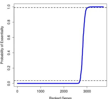
Zi. Genes withZ¯i<0.05are classified as non-essential (i.e. Zi=1in less than 5% of the final sample), and genes with Z¯i>0.95are classified as essential. A total of 757 genes are categorized as essential by this criterion. The remaining genes represent those genes for which the method is unable to reach an essentiality assignment with confidence. Fig-ure 2.3 shows a plot of the sortedZ¯ivalues for all the genes, with the blue lines representing the thresholds of essentiality and non-essentiality. Notice that the majority of genes have a small probability of being essential (i.e. lowZi) which expected in most bacterial genomes.

Table 2.1: Statistics for essentials, non-essentials and uncertain genes. Non-essential genes are those with Zi <0.05, Essential genes are those with Zi >0.95. Average span is in nucleotides.

Total Average

Genes TA Sites Insertions Max Run Span

Essentials 757 20.50 1.87 16.35 969.55

Uncertain 242 17.43 7.50 5.27 400.74

Non-Essentials 2703 15.69 10.77 2.05 55.47

Table 2.1 reports statistics for the different categories of genes. On average essential genes contained significantly longer maximum runs of insertion (16.35) than non-essential genes and these runs spanned a larger number of nucleotides (969.5), which is consistent with our expectations for essentiality. Non-essential genes contained a larger number of insertions on average (15.69). Although essential genes contained only a small

(38)

Figure 2.3: Plot of sortedZi¯ values for all genes. The averageZi of the final sample for all genes was estimated, and plotted in ascending order. The dashed lines represent the respective thresholds for the two categories of essentiality: Z¯i>0.9902andZ¯i<0.0371 number of insertions (1.87) this number was greater than zero, indicating that the method is capable of detecting essential genes with a small number of insertions, provided they contain a long enough run of non-insertions suggestive of an essential region.

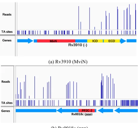
Figure 2.4 contains some examples of those genes with significant runs of non-insertions coinciding with the domain predictions from Pfam. Rv3190 encodes for two C-terminal protein domains (sugar-binding and extracellular domains) and a N-terminal, MviN-like, domain which regulates peptidoglycan biosynthesis and has been shown to be essential for growth in mycobacteria. This protein is actually a flippase of lipid-II and is regulated by interaction with FhaA (Rv0020c), which is phosporylated by PknB [36]. In-sertions in Rv3910 are found only in the C-terminal domains, but not the N-terminal

(39)

mem-(a) Rv3910 (MviN)

(b) Rv0018c (ppp)

Figure 2.4: Example genes with essential domains. Essential domains are indicated in red, and non-essential domains (as predicted by PFAM) are indicated in yellow.

brane domain, implying it alone is necessary for growth. Rv2051c (Ppm1) is involved in cell-wall glycolipid synthesis, an essential role within mycobacteria, and shows evidence of an essential domain (Pfam family: - PF0535.21) within its C-terminus which matches previous analyses of this gene [37]. Rv0018c (serine/threonine phosphatase) contains an essential catalytic domain within its N-terminus, and has been shown to dephosphorylate Rv0020 (FhaA) counteracting phosphorylation by PknB [38]. Transposon insertions are only observed in the extracellular domain of unknown function.

(40)

2.4.2 Concordance with Previous Results

The essentiality of the entireM. tuberculosisgenome has been characterized previ-ously using transposon-site hybridization [11, 12]. We compare our essentiality inferences to previous results to verify that our method achieves results that are consistent with ex-pectations of the essentiality in M. tuberculosis. Sassetti et al. utilized Transposon Site Hybridization (TraSH) to characterize the genes necessary for optimal growthin vitro, for a library of transposon mutants grown on 0.02% glucose and rich-media (7H10). While our method analyzes deep sequencing of transposon libraries, TraSH utilizes hybridization of gene-specific probes to quantify the level of fluorescence being emitted by hybridization probes to determine which genes are being interrupted in the library of mutants. Table 2.2 contains a comparison between the two methods.

Table 2.2: Comparison of essentiality predictions with TraSH analysis. The results ob-tained by Sassetti. et. al are compare with those obob-tained with our Gumbel method for genes inM. tuberculosis. Genes for which the TraSH method did not produce data, are labeled ”no-data”. Genes with less than four TA sites were labeled ”Short” as they could not be analyzed by the Gumbel method.

Gumbel Method

Essential Uncertain Non-Essential Short Total

T raSH (Sassetti) Essentials 457 46 82 29 614 Growth-Defect 11 2 28 1 42 Non-Essential 123 116 2137 144 2520 No-Data 166 78 456 113 813 Total 757 242 2703 287 3989

Sassetti et al. included an additional category of genes representing those whose interruption causes growth-defects (i.e. slower growth); our method does not make this

(41)

distinction. Excluding these, the two methods show agreement in 74.4% of essentials, and 84.8% of non-essentials for a total of 82.8% across both categories. There were only 82 genes predicted to be essential by TraSH but not by our method, and 123 genes predicted to be non-essential by TraSH but found to be essential by our method.

Some of these differences could be due to the different growth conditions of the li-braries. For example, because our library was grown on glycerol we find genes necessary for glycerol metabolism as essential, such as GlpK (glycerol kinase). Other differences may be due to incomplete sequence coverage (e.g. gaps in PE_PGRS genes, which are highly GC-rich and hard to sequence). Two out of 62 PE_PGRS genes in the H37Rv genome were classified as essential by our model because of large regions without inser-tions, though genes in this family are generally believed to be non-essential [39]. Over-representation of PE_PGRS gene among essentials was also noted in other transposon li-brary analyses using sequencing [40].

One notable difference is that Sassetti et al. foundglcBto be non-essential, however insertion pattern clearly indicate that this gene was unable to tolerate insertions in the li-braries of mutants analyzed. GlcB encodes for malate synthase inM. tuberculosis, which was originally thought to be necessary only for growth on fatty-acids as part of a glyoxy-late shunt [41], but has recently been shown to be essential on other carbon sources like dextrose [42]. A complete absence of transposon insertions in Rv1837c was also observed in the DeADMAn studies [40]. Our data suggests that GlcB is also essential for growth on glycerol (in liquid culture with minimal media), showing a significant run of non-insertions

(42)

(25 out of 27 - spanning 2078 nucleotides, p(Zi=1)=1.0). It should be be noted that in the original TraSH data, GlcB had a hybridization ratio of 0.41, which is near the threshold for essentiality (<0.20).

(43)

3 MODELING INDIVIDUAL INSERTION FREQUENCIES

*

3.1 Introduction

One limitation of the Gumbel method introduced in Section 2 is that it assumes a global insertion (or non-insertion) frequency that is shared by all non-essential genes. While this assumption makes the equations manageable, it is unlikely to be true. In reality, losing the function of a gene (by disrupting its function with a transposon) is likely to lead to different fitness costs to the organism depending on the function being disrupted and the biological (metabolic) costs to the organism.

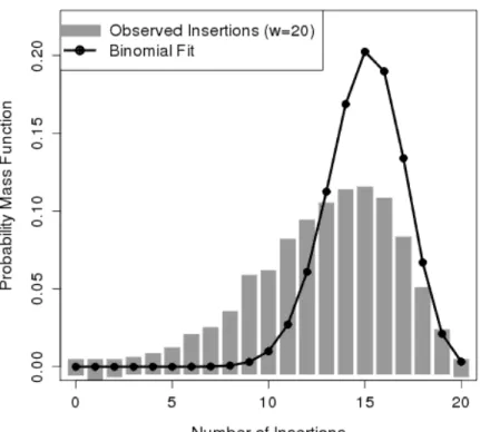
This variability in insertion probability is evident in libraries of transposon mutants. Figure 3.1 shows a histogram of the observed number of insertions within windows of 20 TA sites (gray bars), for a transposon mutant library ofM. tuberculosis[17]. The resulting distribution of the number of insertions is more dispersed than what would be expected with a fitted binomial distribution (black line). This suggests that the insertion frequency is not constant, but instead varies depending on the genomic region being considered. Assuming an insertion probability that is globally constant will ignore this variability, and lead to less reliable predictions.

In this Section a new hierarchical model of essentiality is introduced which over-comes this limitation [26, 27]. This method utilizes a binomial likelihood to model the *_{© 2014 IEEE. Reprinted, with permission, from DeJesus, M.A. and Ioerger, T.R., “Capturing} uncer-tainty by modeling local transposon insertion frequencies improves discrimination of essential genes”, IEEE Transactions on Computational Biology and Bioinformatics, May 2014.

(44)

Figure 3.1: Histogram of the number of insertions within windows of 20 TA sites (gray bars). A beta-binomial model with a variable insertion frequency is capable of fitting the observed data (black line).

(45)

insertions within the genes. As with the Gumbel model, insertions are treated as Bernoulli events with a probability of success representing the insertion probability. This insertion probability, however, is allowed to be different for each gene.

The Bayesian framework on which these models is based on allows for a hierarchical extension by applying a prior distributions on the parameters of interest. This hierarchical approached improves the prediction of essential genes by taking into consideration the natural variability of insertion probabilities observed in the data as well as the length of the genes into account. Section 3.2 describes the model in detail, while Sections 3.3 and Section 3.4 briefly goes over the parameter estimation and results.

3.2 Hierarchical Model

For the all genes i∈ {1...G}, letYi ={ki,ni} represent the data for thei-th gene, consisting of the number of insertions,ki, and the total number of TA sites,ni. Each gene icontains a latent variableθi, which represents the insertion probability for this gene. The genes are modeled as a mixture of non-essential and essential genes, with an indicator variable,Zi={0,1}, indicating whether thei-th gene belongs to the class of non-essential (0) or essential (1) genes. The mixture coefficient,ω1, represents the probability of a gene

belonging to the essential class (with the probability of belonging to the non-essential class ω0=1−ω1).

(46)

3.2.1 Complete Data Likelihood

For each genei, the likelihood of observingkiinsertions out ofni TA sites is given by a binomial distribution with success probabilityθi. Assuming genes are independent of each other, the complete data likelihood is given by the product of binomial distributions over all the genes:

G

∏

i

Binomial(ki|ni,θi) (3.1)

3.2.2 Prior Probabilities

The distribution of individual insertion probabilities,θiis modeled by a mixture of two Beta distributions: one modeling the probability of insertion for “essential” genes, and another modeling the insertion probability at non-essential genes:

θi|Zi=0∼Beta(κ0ρ0, κ0(1−ρ0))

θi|Zi=1∼Beta(κ1ρ1, κ1(1−ρ1))

(3.2)

Under this parameterization (i.e. α =κρ andβ =κ(1−ρ)), theρ parameter represents the mean insertion probability (i.e. mean of the distribution). On the other hand, theκ parameter can be thought of as the number of observations. This is because in the common parameterization the sum α+β can represent the number of Bernoulli trials depending on the application. Under this parameterizationα+β =κρ+κ(1−ρ) =κ. Thus, with larger values ofκ the distribution becomes tighter around the mean (i.e. ρ).

(47)

range[0,1], Beta distributions are chosen as priors:

ρ0∼Beta(α0,β0)

ρ1∼Beta(α1,β1)

(3.3)

whereα0,β0,α1, andβ1are hyper-parameters for the beta distribution.

As theκ parameters require support for values in the range[0,inf), gamma distribu-tions are chosen as priors:

κ0∼Gamma(a0,b0)

κ1∼Gamma(a1,b1)

(3.4)

where a0, b0, a1, andb1 are hyper-parameters describing the shape and and scale of the

respective distributions.

The prior distribution for the indicator variable,Zi, is given by the Bernoulli distribu-tion, with probability of successω1, which represents the probability of a gene belonging

to the class of essential genes:

Zi∼Bernoulli(ω1) (3.5)

Finally, the prior distribution forω1is given by a Beta distribution:

(48)

3.3 Parameter Estimation

3.3.1 Conditional Distributions

Below, the conditional distributions for the parameters of the essential genes are given (the corresponding distributions for the non-essential parameters are defined in a similar manner). For an individual insertion probability, the conditional distribution is a beta distribution with updated parameters:

p(θi|ki,κ,ρ,Zi=1)∝Beta(θi|κ1ρ1+ki, κ1(1−ρ1) +ni−ki)

The beta distributions depend on parametersρ1andκ1which are distributed as

fol-lows:

p(κ1|ki,θi,ρ1,Zi=1) (3.7)

∝Beta(θi|κ1ρ1, κ1(1−ρ1))×Gamma(κ|a1,b1) (3.8)

p(ρ1|ki,θi,κ1,Zi=1) (3.9)

∝Beta(θi|κ1ρ1, κ1(1−ρ1))×Beta(ρ1|α1,β1) (3.10)

Finally, the individual indicator variable,Zi, is given by a Bernoulli distribution:

p(Zi=1|ki,θi,κ1,ρ1,ω1) =Bernoulli

(

p1

p1+p0

(49)

where,

p1=Beta(θi|κ1ρ1+ki, κ1(1−ρ1) +ni−ki)×ω1

p0=Beta(θi|κ0ρ0+ki, κ0(1−ρ0) +ni−ki)×(1−ω1)

3.3.2 Metropolis-Hastings

As with the Gumbel model, parameters are estimated using MCMC samples obtained through the Metropolis-Hastings algorithm. Because the binomial likelihood (3.1) and the beta priors (3.2) are conjugate, the resulting conditional distribution can be sampled from directly. This is a special case of the Metropolis-Hastings algorithm called the Gibbs Sampler, where the proposal density is always accepted, and thus the MH ratio will never be rejected.

However, this is not the case for the conditional distributions of theρandκ parame-ters (Equations (3.10) and (3.8)), therefore the Metropolis Hastings algorithm is necessary to sample from these (non-standard) distributions. A combination of Gibbs Steps and MH steps can be used obtain samples for all the parameters (See Algorithm 2).

3.4 Results

Our method was applied to deep-sequencing data from mutant libraries of the H37Rv strain of M. tuberculosis [17, 25]. The library was grown in minimal media and 0.1% glycerol. The surviving mutants were sequenced with an Illumina GAII sequencer, with a read length of 36 bp, producing 6 to 8 million reads. These reads were mapped to the

(50)

Algorithm:Random-Walk Metropolis-Hastings

Result:MCMC Samples of the densities p(Zi|Y,Θ,ρ,κ)andp(θi|Y,ρ,κ)for i∈ {1...G}

Assign starting values toθi,ρ0,κ0,ρ1,κ1and initializeZibased on proportion of

insertions within individual genes.

forj=1 to desired sample sizedo //Gibbs Steps -θi

fori←1toGdo

Sampleθi∼Beta(ρκ+ki,κ(1−ρ) +ni−ki) end

//MH Step -ρ0

Draw candidate parameterρ₀cfrom Normal distribution, N(ρ₀j−1,v) and accept according to MH ratio f(ρ

c 0)

f(ρ₀i−1) //MH Step -κ0

Draw candidate parameterκ₀cfrom Normal distribution, N(κ₀j−1,v) and accept according to MH ratio f(κ

c 0)

f(κ₀i−1) //MH Step -ρ1

Draw candidate parameterρ₁cfrom Normal distribution, N(ρ₁j−1,v) and accept according to MH ratio f(ρ

c 1)

f(ρ₁i−1) //MH Step -κ1

Draw candidate parameterκ₁cfrom Normal distribution, N(κ₁j−1,v) and accept according to MH ratio f(κ

c 1)

f(κ₁i−1)

LetKz equal the number of genes withZ_ij=1 LetGbe the total number of genes

Sampleω₁(j)∼Beta(αw+Kz,βw+G−Kz) //Gibbs Steps -Zi fori←1toGdo p1= p(ki|Zi=0,ρ1,κ1)×ω1 p0= p(ki|Zi=0,ρ0,κ0)×(1−ω1) SampleZ_i(j)∼Bernoulli( p1 p1+p0) end end

Algorithm 2:Random-Walk Metropolis-Hastings Algorithm for Sampling values ofθi andZifor all genesi

(51)

H37Rv genome, producing read counts at each TA site in the genome.

The H37Rv genome is 4.41 million bp long and contains 3,989 open-reading frames (ORFs) [35]. Of these ORFs, 3947 contain at least 1 TA site, with an average of 15.9 TA sites per ORF. The remaining 42 ORFs, which do not contain a TA site, were not considered in this analysis as their essentiality cannot be determined with libraries built with the Himar1 transposon.

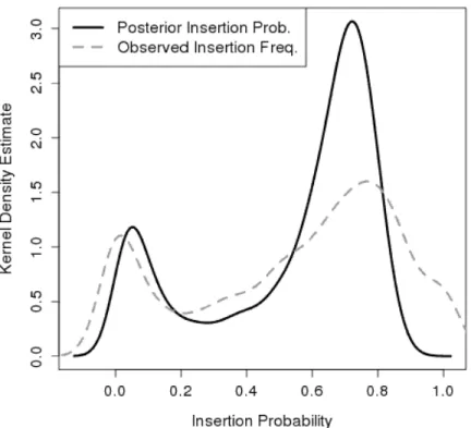
Figure 3.2: Kernel density estimates for the mean posterior insertion probability (black-solid) and observed insertion frequency (gray-dashed) for all the genes.

A sample of 52,000 values was obtained with the independent Metropolis Hastings algorithm. In order to make sure that the MCMC chain converged before parameters were estimated, the first 2,000 samples were discarded as part of the burn-in period. The re-maining 50,000 samples were used to estimate the posterior mean of the parameters of the

(52)

model.

3.4.1 Insertion Frequencies

Samples of the individual probabilities were obtained for all genes. The mean inser-tion frequency, θ¯i, was estimated from these samples. Figure 3.2 contains a density plot of the mean insertion probability (black-line). The plot shows two peaks (θ =0.052and θ =0.721) corresponding to the mixture of essential and non-essential genes. For compar-ison, the insertion frequency observed in the data (i.e. ki

ni) is plotted as well (gray dashed

line). The mean insertion probability resembles the observed frequency, with sharper peaks at the posterior modes.

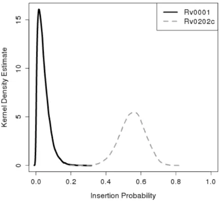
Figure 3.3: Kernel density estimates for the posterior insertion probability of DnaA (Rv0001), a known essential gene involved in DNA repair, and MmpL11 (Rv0202c), a known non-essential gene believed to function as a transmembrane protein.

(53)

The samples of insertion probability for the genes reflect our expectations for es-sential and non-eses-sential genes. Figure 3.3 shows density plots of the samples for DnaA (Rv0001) and MmpL11 (Rv0202c). DnaA is a known essential gene involved in DNA repair. It contains a total of 32 TA sites with a single insertion in the C-terminus. Its mean insertion probability isθi¯ =0.044, corresponding to the small probability of observing an insertion in this essential gene. On the other hand, MmpL11 is a transmembrane transport protein determined to be non-essential in knock-out experiments [43]. It contains inser-tions in 20 out of 39 TA sites, with a mean insertion probability ofθi¯ =0.551, consistent with expectations of non-essential genes.

3.4.2 Essentiality Results

To estimate the probability of a gene being essential, the sample of individual es-sentiality values,Zi, was averaged for all genes (Z¯i= 1_n∑Zi). A method analogous to the Benjamini-Hochberg procedure for posterior probabilities was used to obtain the thresh-olds of essentiality [44]. Setting the False Discovery Rate at 5%, genes withZ¯i>0.99304 are classified as essential, and genes withZ¯i<0.0391are classified as non-essential. Those genes that do not meet these thresholds are classified as Uncertain.

Comparison to the TraSH Method

The essentiality of the M. tuberculosis genome has been assessed before, through the Transposon Site Hybridization method [11, 12]. This method quantifies the amount of luminescence that is observed in probes that hybridize to each of the genes in the genome [10]. Hybridization ratios were obtained from libraries of M. tuberculosisgrown in rich