2011
Novel data clustering methods and applications
Sijia Liu
Iowa State University
Follow this and additional works at:
https://lib.dr.iastate.edu/etd
Part of the
Mathematics Commons
This Dissertation is brought to you for free and open access by the Iowa State University Capstones, Theses and Dissertations at Iowa State University Digital Repository. It has been accepted for inclusion in Graduate Theses and Dissertations by an authorized administrator of Iowa State University Digital Repository. For more information, please [email protected].
Recommended Citation
Liu, Sijia, "Novel data clustering methods and applications" (2011).Graduate Theses and Dissertations. 10206.
by
Sijia Liu
A dissertation submitted to the graduate faculty in partial fulfillment of the requirements for the degree of
DOCTOR OF PHILOSOPHY
Major: Applied Mathematics
Program of Study Committee: Anastasios Matzavinos, Major Professor
Paul Sacks Jim W. Evans Sunder Sethuraman Alexander Roitershtein
Iowa State University Ames, Iowa
2011
TABLE OF CONTENTS LIST OF TABLES . . . iv LIST OF FIGURES . . . v ACKNOWLEDGEMENTS . . . viii ABSTRACT . . . x CHAPTER 1. Introduction . . . 1
1.1 Centroid-based clustering methods . . . 2
1.2 Outline of the thesis . . . 4
CHAPTER 2. K-Means Method and Fuzzy C-Means Method . . . 6
2.1 Introduction . . . 6
2.2 K-Means Method and Fuzzy C-Means Method . . . 7
2.3 K-Means Method and Principal Component Analysis . . . 9
2.4 Extensions and Variants of K-Means Method . . . 15
2.4.1 Kernel Based Fuzzy Clustering with Spatial Constraints . . . 15
2.4.2 The Extension of K-means Method for Overlapping Clustering . . . 22
CHAPTER 3. Spectral Clustering Methods . . . 26
3.1 Introduction . . . 26
3.2 The Derivations and Algorithms of Spectral Clustering Methods . . . 27
3.2.1 Graph Cut and Spectral Clustering . . . 28
3.2.2 Random Walks and Spectral Clustering . . . 37
3.2.3 Perturbation Theory and Spectral Clustering . . . 39
3.3 Applications . . . 50
3.3.1 Image Segmentation and Shape Recognition . . . 50
3.4 Learning Spectral Clustering Methods . . . 60
3.4.1 Learning Spectral Clustering . . . 60
CHAPTER 4. Novel Data Clustering Method Fuzzy-RW . . . 65
4.1 Distances Defined by Random Walks on the Graph . . . 66
4.2 Incorporating the Distance Defined by Random Walks in the FCM Framework with Penalty Term . . . 71
4.3 Utilizing the Local Properties of Datasets in the Weight Matrix . . . 73
4.4 Clustering With Directional Preference . . . 75
4.5 Local PCA Induced Automatic Adaptive Clustering . . . 79
CHAPTER 5. Face Recognition . . . 84
5.1 Face Recognition by Using Lower Dimensional Linear Subspaces . . . 84
5.1.1 Approximation of the Illumination Cones by Harmonic Basis . . . 86
5.1.2 Acquiring Subspaces Under Variable Lighting Conditions For Face Recog-nition . . . 92
5.2 Appearance-Based Face Recognition . . . 96
5.2.1 Face Recognition by Eigenfaces . . . 97
5.2.2 Face Recognition by Fisherfaces . . . 98
5.2.3 Face Recognition by Laplacianfaces . . . 101
5.3 Incorporating Fuzzy-RW Into Face Recognition Algorithms . . . 104
BIBLIOGRAPHY . . . 110
LIST OF TABLES
Table 2.1 Algorithm of the K-means method . . . 8
Table 2.2 Algorithm of the fuzzy c-means method . . . 10
Table 2.3 Image segmentation by the kernel-based fuzzy c-means method with spatial constraints (SKFCM) . . . 21
Table 2.4 Multiple Assignment of A Data Point . . . 24
Table 2.5 OKM Algorithm . . . 25
Table 3.1 Learning Spectral Clustering Algorithm . . . 63
Table 4.1 The true positive (TP) and false positive (FP) rates obtained by apply-ing FCM, spectral method, FLAME, and Fuzzy-RW respectively. (See text for the parameters used for each algorithm.) . . . 77
LIST OF FIGURES
Figure 2.1 (a). A dataset that consists of four groups of data points. Each group of data points are of Gaussian distribution. (b). The clustering result by applying K-means method and requiring the number of clusters to be four. Different clusters are colored with red, blue, green, and magenta. Centroids of clusters are marked with black circles. . . 8
Figure 2.2 (a) The original image, (b-e) Color segmentation results by applying fuzzy c-means method. In each result, the assignments of pixels are based on their maximum membership values. The number of clusters in the results are required to be K = 3, K = 4, K = 5, and K = 6 respectively. . . 15
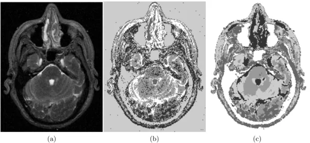
Figure 2.3 Results of segmentation on a magnetic resonance image corrupted by Gaussian noise with mean 0 and variance 0.0009. (a). The corrupted image. (b). Segmentation result obtained by applying fuzzy c-means method with 5 clusters. (c). Segmentation result obtained by applying SKFCM with 5 clusters. The parameters that used to obtain the results can be found in the text. . . 21
Figure 3.1 From (a) to (d): original images. From (e) to (h): segmentation results obtained by using normalized spectral clustering algorithm. . . 52
Figure 3.2 Image segmentation results given by multi-scale spectral segmentation method Cour et al. (2005a). left column: original images. right column: segmentation results obtained by requiring the number of clusters to be 40, 45, and 40 respectively. . . 59
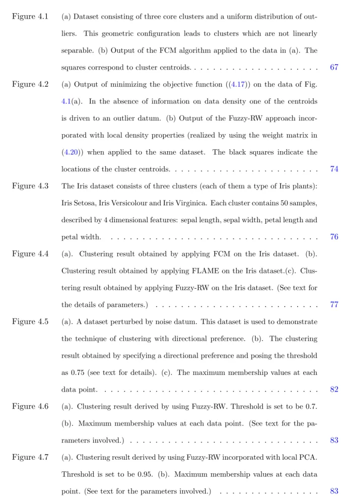
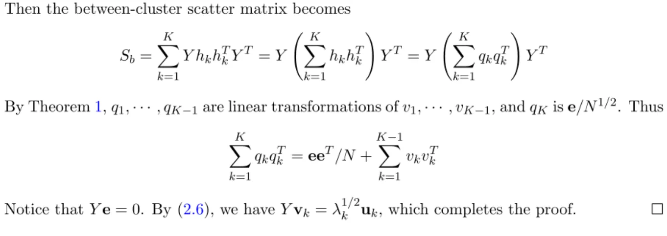
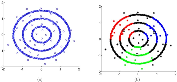
Figure 4.1 (a) Dataset consisting of three core clusters and a uniform distribution of out-liers. This geometric configuration leads to clusters which are not linearly separable. (b) Output of the FCM algorithm applied to the data in (a). The squares correspond to cluster centroids.. . . 67
Figure 4.2 (a) Output of minimizing the objective function ((4.17)) on the data of Fig.
4.1(a). In the absence of information on data density one of the centroids is driven to an outlier datum. (b) Output of the Fuzzy-RW approach incor-porated with local density properties (realized by using the weight matrix in (4.20)) when applied to the same dataset. The black squares indicate the locations of the cluster centroids. . . 74
Figure 4.3 The Iris dataset consists of three clusters (each of them a type of Iris plants): Iris Setosa, Iris Versicolour and Iris Virginica. Each cluster contains 50 samples, described by 4 dimensional features: sepal length, sepal width, petal length and petal width. . . 76
Figure 4.4 (a). Clustering result obtained by applying FCM on the Iris dataset. (b). Clustering result obtained by applying FLAME on the Iris dataset.(c). Clus-tering result obtained by applying Fuzzy-RW on the Iris dataset. (See text for the details of parameters.) . . . 77
Figure 4.5 (a). A dataset perturbed by noise datum. This dataset is used to demonstrate the technique of clustering with directional preference. (b). The clustering result obtained by specifying a directional preference and posing the threshold as 0.75 (see text for details). (c). The maximum membership values at each data point. . . 82
Figure 4.6 (a). Clustering result derived by using Fuzzy-RW. Threshold is set to be 0.7. (b). Maximum membership values at each data point. (See text for the pa-rameters involved.) . . . 83
Figure 4.7 (a). Clustering result derived by using Fuzzy-RW incorporated with local PCA. Threshold is set to be 0.95. (b). Maximum membership values at each data point. (See text for the parameters involved.) . . . 83
Figure 5.1 Training set consists of 75 images. From (a) to (c), the dimensionality reduction is done by using the eigenface technology. (a). Result given by FCM with the number of clusters set to be 15. (b). Result given by spectral clustering with weight matrix defined as Wij = exp (−||xi−xj||2/σ) with σ = 20000. K-Means method is applied on the eigenvectors that correspond to the smallest 15 nonzero eigenvalues of the graph Laplacian. (c). Result given by Fuzzy-RW with commute distance,σ= 127.6,r= 22.6,s = 2, γ= 1/6, and K = 1038. (d). Result given by first reducing the dimensionality using the Laplacianfaces technology then applying Fuzzy-RW with commute distance. The parameters used in Fuzzy-RW areσ= 51,γ= 0 andK= 1040. . . . . 108 Figure 5.2 (a). The clustering result on the training set T. This result is generated by
using σh∗ learnt fromT, and among the rangeH. (See the text for details.)
(b). The face recognition results of the whole Yale Database using Fuzzy-RW withσh∗ and absorption distances. (See text for details of parameters.) . . . 109
Figure 5.3 (a). Face recognition results on the test setX1=X\T1. (b). Face recognition results on the test setX2=X\T2. (See text for details of relative parameters.) 109
ACKNOWLEDGEMENTS
It is my pleasure to express my gratitude to my advisor, Dr. Anastasios Matzavinos, for his continuous support, motivation, encouragement, and help during my Ph.D. study and research. Without his help, this thesis would not be possible. With his guidance, I started to learn how to do research and how to grow academically with collaborative spirit. With his motivation and encouragement, I started to explore the strength of innovation.
I would like to thank Dr. Sunder Sethuraman, with whom I have collaborated on the research of data clustering. The collaboration experience showed me the joint strength of theo-retical and problem driven research. I want to give my gratitude to Dr. Alexander Roitershtein. It has been an educational and interesting experience to collaborate with him. I am also grate-ful to all my other collaborators for their help.
I owe my gratitude to Dr. Paul Sacks, Dr. James Evans, and Dr. Howard Levine, who have given me generous help and encouragement. Dr. Sacks has been overseeing my study and research as the Director of Graduate Education in Department of Mathematics, and has given invaluable guidance and support in critical situations. Dr. Levine has trusted my ability, encouraged me and kept me motivated to overcome difficulties. Dr. Evans has shown me a broad view of applications of mathematics in physics and chemistry.
I am given the opportunity to pursue the Ph.D. degree by the Department of Mathematics, Iowa State University, to whom I owe my sincere gratitude. I would like to thank all my friends for supporting me and spending the five years with me.
me, and supports me. Without his help, I could not be able to focus almost all my energy to solve challenging problems, to regenerate from setbacks, and to be optimistic even when I am facing difficulties.
I want to thank my family, especially my parents, Bianxia Duan and Bing Liu, for giving birth to me, for nurturing and educating me, for having faith in me, and for their constant care and support throughout my life. My grandfather, Jiantang Liang, has been educating me since I was young. Last but not least, I would like to give special thanks to my grandmother, Xiulan Xia, who had the kindest heart and will always be with me in my heart.
ABSTRACT
The need to interpret and extract possible inferences from high-dimensional datasets has led over the past decades to the development of dimensionality reduction and data cluster-ing techniques. Scientific and technological applications of clustercluster-ing methodologies include among others bioinformatics, biomedical image analysis and biological data mining. Current research in data clustering focuses on identifying and exploiting information on dataset ge-ometry and on developing robust algorithms for noisy datasets. Recent approaches based on spectral graph theory have been devised to efficiently handle dataset geometries exhibiting a manifold structure, and fuzzy clustering methods have been developed that assign cluster membership probabilities to data that cannot be readily assigned to a specific cluster.
In this thesis, we develop a family of new data clustering algorithms that combine the strengths of existing spectral approaches to clustering with various desirable properties of fuzzy methods. More precisely, we consider a slate of “random-walk” distances arising in the context of several weighted graphs formed from the data set, which allow to assign “fuzzy” variables to data points which respect in many ways their geometry. The developed methodology groups together data which are in a sense “well-connected”, as in spectral clustering, but also assigns to them membership values as in other commonly used fuzzy clustering approaches. This approach is very well suited for image analysis applications and, in particular, we use it to develop a novel facial recognition system that outperforms other well-established methods.
CHAPTER 1. Introduction
The need to interpret and extract possible inferences from high-dimensional datasets has led over the past decades to the development of dimensionality reduction and data clustering techniques Filippone et al. (2007). Scientific and technological applications of such clustering methodologies include among others computer imaging Archip et al. (2005) Shi and Malik (2000), data mining and bioinformatics Liao et al. (2009) Snel et al. (2002). One of the most widely used and studied statistical methods for data clustering is the K-means algorithm, which was first introduced in MacQueen (1967) and is still in use nowadays as the prototypical example of a non-overlapping clustering approach Kogan (2007). The applicability of the K -means algorithm, however, is restricted by the requirement that the clusters to be identified should be well-separated and of a regular, convex-shaped geometry, a requirement that is often not met in practice. In this context, two fundamentally distinct approaches have been proposed in the past to address these restrictions.
Bezdek et al. Bezdek et al. (1984) proposed the fuzzy c-means (FCM) algorithm as an alternative, soft clustering approach that generates fuzzy partitions for a given dataset. In the case of FCM the clusters to be identified do not have to be well-separated, as the method assigns cluster membership probabilities to undecidable elements of the dataset that cannot be readily assigned to a specific cluster. However, the method does not exploit the intrinsic geometry of non-convex clusters, and its performance is drastically reduced when applied to datasets that are curved, elongated or contain clusters of different dispersion. This behaviour can also be observed in the case of the standardK-means algorithm Ng et al. (2001). Although these algorithms have been successful in a number of examples, this thesis focuses on datasets for which their performance is poor.
the computational problems associated with the geometry of datasets exhibiting a manifold structure. Such approaches exploit the information encoded in the spectrum of specific linear operators acting on the data, such as the normalized graph Laplacian. The effectiveness of such spectral methodologies has been attributed to the analogy that exists between the graph Laplacian and the Beltrami operator Rosenberg (1997). The latter is defined in Chapter 3 and it provides the means for describing the process of diffusion on Riemannian manifolds and can consequently be used to identify the optimal embedding dimension, which in turn has natural connections to clustering Belkin and Niyogi (2003). As discussed in Chapters 3 and 4, an alternative analysis focuses on the properties of the normalized graph Laplacian as a stochastic matrix. The eigenvalues of the latter represent the various time scales of the corresponding random walk, and this information can be used to identify efficient representations of the underlying dataset, hence facilitating the process of clustering Coifman and Lafon (2006). In the following, we define the basic mathematical notions underlying clustering methods, such as the ones described above, and delineate the contents of this thesis.
1.1 Centroid-based clustering methods
We introduce here some of the basic notions underlying the classical k-means and fuzzyc -means methods. More details are provided in Chapter 2, and the spectral clustering approach is introduced in Chapter 3. In what follows, we consider a set of data
D={x1, x2, . . . , xn} ⊂Rm.
embedded in a Euclidean space. The output of a data clustering algorithm is a partition:
Π ={π1, π2, . . . , πk}, (1.1)
wherek≤nand each πi is a nonempty subset ofD. Π is a partition of Din the sense that
[
i≤k
πi =D and πi∩πj =∅for all i6=j. (1.2)
In this context, the elements of Π are usually referred to as clusters. In practice, one is interested in partitions of D that satisfy specific requirements, usually expressed in terms of a distance functiond(·,·) that is defined on the background Euclidean space.
The classicalk-means algorithm is based on reducing the notion of a clusterπi to that of a
cluster representative or centroidc(πi) according to the relation
c(πi) = arg min ( X x∈πi d(x, y) y∈R m ) . (1.3)
In its simplest form,k-means consists of initializing a random partition of Dand subsequently updating iteratively the partition Π and the centroids {c(πi)}i≤k through the following two
steps (see, e.g., Kogan (2007)):
(a) Given{πi}i≤k, update{c(πi)}i≤k according to (1.3).
(b) Given{c(πi)}i≤k, update{πi}i≤k according to centroid proximity, i.e., for eachi≤k,
πi =
x∈ D |d(ci, x)≤d(cj, x) for each j≤k
In applications, it is often desirable to relax condition (1.2) in order to accommodate for overlapping clusters Fu and Medico (2007). Moreover, condition (1.2) can be too restrictive in the context of filtering data outliers that are not associated with any of the clusters present in the data set. These restrictions are overcome by fuzzy clustering approaches that allow the determination of outliers in the data and accommodate multiple membership of data to different clusters Ma; and Wu (2007).
In order to introduce fuzzy clustering algorithms, we reformulate condition (1.2) as:
uij ∈ {0,1}, k X `=1 u`j = 1, and n X `=1 ui`>0, (1.4)
for all i ≤ k and j ≤ n, where uij denotes the membership of datum xj to cluster πi (i.e.,
uij = 1 ifxj ∈πi, and uij = 0 ifxj ∈/ πi). The matrix (uij)i≤k,j≤n is usually referred to as the
data membership matrix. In fuzzy clustering approaches,uij is allowed to range in the interval
[0,1] and condition (1.4) is replaced by:
uij ∈[0,1], k X `=1 u`j = 1, and n X `=1 ui`>0, (1.5)
for all i ≤ k and j ≤ n Bezdek et al. (1984). In light of Eq. (1.5), the matrix (uij)i≤k,j≤n
a probability distribution with uij denoting the probability of data point xj being associated
with cluster πi. Hence, fuzzy clustering approaches are characterized by a shift in emphasis
from defining clusters and assigning data points to them to that of a membership probability distribution.
The prototypical example of a fuzzy clustering algorithm is the fuzzy c-means method (FCM) developed by Bezdeket al. Bezdek et al. (1984). The FCM algorithm can be formulated as an optimization method for the objective function Jp, given by:
Jp(U, C) = k X i=1 n X j=1 upijkxj−cik2, (1.6)
where U = (uij)i≤k,j≤n is a fuzzy partition matrix, i.e. its entries satisfy condition (1.5), and
C = (ci)i≤k is the matrix of cluster centroids ci ∈Rm. The real number p is a “fuzzification”
parameter weighting the contribution of the membership probabilities to Jp Bezdek et al.
(1984). In general, depending on the specific application and the nature of the data, a number of different choices can be made on the norm k · k. The FCM approach consists of globally minimizing Jp for somep > 1 over the set of fuzzy partition matrices U and cluster centroids
C. The minimization procedure that is usually employed in this context involves an alternating directions scheme Ma; and Wu (2007), which is commonly referred to as the FCM algorithm. A listing of the FCM algorithm is given in Chapter 2.
This approach, albeit conceptually simple, works remarkably well in identifying clusters, the convex hulls of which do not intersect Jain (2008) Meila (2006), with a representative example being discussed in Chapter 2. However, for general data sets, Jp is not convex and, as we
demonstrate in Chapter 3, one can readily construct data setsD for which the standard FCM algorithm fails to detect the global minimum ofJp Ng et al. (2001).
1.2 Outline of the thesis
In this thesis, we consider a slate of “random-walk” distances arising in the context of several weighted graphs formed from the data set, in a comprehensive generalized FCM frame-work, which allow to assign “fuzzy” variables to data points which respect in many ways their geometry. The method we present groups together data which are in a sense “well-connected”,
as in spectral clustering, but also assigns to them membership values as in FCM. We remark our technique is different than say clustering by spectral methods, and then applying FCM. It is also much different than other recent approaches in the literature, such as the FLAME Fu and Medico (2007) and DIFFUZZY Cominetti et al. (2010) algorithms, which compute “core clusters” and try to assign data points to them.
The particular random walk distance focused upon in the thesis, among others, is the “absorption” distance, which is new to the literature (see Chapter 4 for definitions). We remark, however, a few years ago a “commute-time” random walk distance was introduced and used in terms of clustering Yen et al. (2005). In a sense, although our technique is more general and works much differently than the approach in Yen et al. (2005), our method builds upon the work in Yen et al. (2005) in terms of using a random walk distance. In particular, in Chapter 4, we introduce novelties, such as motivated “penalty terms” and “locally adaptive” weights to construct underlying graphs from the given data set, which make Fuzzy-RW impervious to random seed initializations.
The outline of the thesis is the following. First, in Chapter 2, we further discuss the classical FCM algorithm, and delineate some of its merits and demerits with respect to some data sets, including some applications to image segmentation and other image analysis tasks. In Chapter 3, we review the various existing approaches to spectral clustering and machine learning approaches. Chapters 2 and 3 culminate in the development of a family of new clustering methods, dubbed Fuzzy-RW, in Chapter 4 which is one of the two main novelties of this thesis. We demonstrate the effectiveness and robustness of Fuzzy-RW on several standard synthetic benchmarks and other standard data sets such as the IRIS and the YALE face data sets Georghiades et al. (2000) in Chapters 4 and 5. In particular, in Chapter 5 we turn our focus on an important application of data clustering, namely the problem of face recognition. After reviewing current approaches and methodologies, we demonstrate that the performance of Fuzzy-RW in face identification is comparable to, and often better than, the performance of existing methods.
CHAPTER 2. K-Means Method and Fuzzy C-Means Method
2.1 Introduction
The K-means method is considered as one of the most popular and standard clustering methods. Although it was initially discovered more than 50 years ago Steinhaus (1956) Lloyd (1982) Ball and Hall (1965) MacQueen (1967) and since then there has been enormous improved techniques designed targeting a variety of applications (see Jain (2008) for a review), the K-means method is still generally applied because of its simplicity and efficiency. The goal of K-means is to partition a given dataset such that data points in a same cluster are similar and the data points in different clusters are dissimilar. It also requires that the clusters are non-overlapping. The clustering algorithms that satisfy the above requirements are classified as crisp data clustering methods. On the other hand, algorithms that allow every data point to be assigned to more than one clusters are classified as fuzzy clustering methods. Fuzzy c-means method, proposed in Dunn (1973) and improved in Bezdek (1981), is a fuzzy clustering method that is analogous to the K-means method. The K-means method and fuzzy c-means method can be varied or improved by being applied with different choices of distance measures Mao and Jain (1996) Linde et al. (1980) Banerjee et al. (2005b), and can be combined with other clustering techniques, for example, kernel methods Zhang et al. (2003), to achieve better results according to the nature of clustering problems. In this chapter, we discuss the K-means method, fuzzy c-means method and their related variants. Section 1 describes the K-means method and fuzzy c-means method. Section 2 discusses the relationship between the K-means method and the principal component analysis. Finally, section 3 describes several extended algorithms based on or related to the K-means and fuzzy c-means method.
2.2 K-Means Method and Fuzzy C-Means Method
For a given datasetX ={xj}N
j=1to be partitioned intoKnon-overlapping clustersC1, C2,· · · , CK,
K-means method aims at finding an optimal partition such that the total distance between data points and the centroids of the clusters to which they are partitioned is minimized. Such a partition is found by minimizing the following objective function:
J = K X i=1 X xj∈Ci kxj−mik2 (2.1)
where k · krepresents the measure of distance, it is proposed as the Euclidean distance in the K-means method. mi is the centroid of the i-th cluster.
However, the problem of finding the globally minimized objective function J is NP-hard Drineas et al. (2004). Instead, a partition can be generated by an iterative algorithm. This algorithm can be initiated with a random partition of X, then it iterates between calculating the centroids of the current partition and updating the partition by assigning data points to their nearest centroids. The K-means algorithm can be summarized in Table 2.1.
The above algorithm can only lead to a local minimum of J, thus the clustering result of the K-means method depends on the partition used for initiation. To reduce the influence of the initial partition on the clustering result, one can run the algorithm multiple times using different randomly generated initial partitions and then choose the result that has the smallest total squared distance Jain (2008). See Fig. 2.1 for an example of applying K-means method to cluster a dataset consisting of four groups of data points that have Gaussian distributions.
Fuzzy c-means method, on the other hand, approaches the problem of clustering X intoK clusters by assigning each data point membership values as the possibilities for it to be classified into multiple clusters. It requires to minimize the total weighted distance between data points and all centroids, where the weights are the corresponding membership values. The objective
Table 2.1: Algorithm of the K-means method
Input: Dataset X ={xj}N
j=1, the number of clusters K, and a small positive value
or the maximum iteration timeT.
Output: A partitionC1, C2,· · · , CK that satisfies∪Ki=1Ci=X andCi∩Cj =∅,∀i6=j. Initiation: Randomly generate a partition{Ci(0)}K
i=1 of X. Iteration:
1. Fori∈ {1,2,· · ·, K}, compute the centroidm(t)i of thei-th clusterCi(t). Compute the objective function
J(t) = K X i=1 X xj∈Ci(t) kxj−m(t)i k2
2. For a data point xj, find its nearest centroid m(t)j∗, i.e.
m(t)j∗ = arg min{kxj −m (t) i k : m (t) i ∈ {m (t) i } K i=1}
Assign xj into the j∗-th cluster for all j ∈ {1,2,· · ·, N} to form a new partition{Ci(t+1)}K
i=1.
3. Repeat the above steps 1) and 2) untilkJ(t+1)−J(t)k< or the iteration time exceedsT.
Figure 2.1: (a). A dataset that consists of four groups of data points. Each group of data points are of Gaussian distribution. (b). The clustering result by applying K-means method and requiring the number of clusters to be four. Different clusters are colored with red, blue, green, and magenta. Centroids of clusters are marked with black circles.
function that fuzzy c-means tries to minimize is the following: Jm= C X i=1 N X j=1 Uijmkxj −mik2 (2.2)
where Uij is the membership value of data point xj to be assigned to thei-th cluster, which
satisfies the requirements
Uij ∈[0,1], ∀i, j, and K X
i=1
Uij = 1, ∀j ∈ {1,· · ·, N} (2.3)
Also, m is the degree of fuzzification Bezdek et al. (2005) that adjusts the effect of the mem-bership values, 1 ≤ m < ∞. Usually m is taken as 2 for simplicity. Fuzzy c-means can be considered as a generalization of the K-means method in the sense that, if we assign each data point into only one cluster and Uij = 1 if and only if xj is assigned to the i-th cluster, the
aboveJm is the same as the objective functionJ in the K-means method.
Similar to the K-means method, an iterative algorithm derived by using the method of Lagrange multiplier can be applied to find a local minimization of Jm for a given a random
initiation. The algorithm can be summarized in Table 3.1.
The measure of distances used in the objective functions of the K-means method and the fuzzy c-means method are not restricted to the Euclidean distance. For example, the K-means method has been combined with the Itakura-Saito distance Linde et al. (1980), a family of Bregman distance Banerjee et al. (2005b). And the fuzzy c-means method has been combined with the kernel methods to cluster datasets that have complex nonlinear structures Zhang et al. (2003).
2.3 K-Means Method and Principal Component Analysis
Principal component analysis (PCA) is a standard unsupervised dimension reduction method that has been broadly used, while K-means method is a popular and efficient unsupervised clus-tering method. It is proved that the principal components obtained from PCA are the
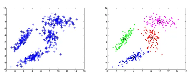
contin-Table 2.2: Algorithm of the fuzzy c-means method
Input Dataset X = {xj}N
j=1, the number of clusters K, and a small positive value
or the maximum iteration timeT.
Output A membership matrix U, where Uij represents the probability to assign xj to
thei-th cluster.
Initiation Randomly generate a membership matrix U0 that satisfies requirements in (2.3).
Iteration
1. Fori∈ {1,2,· · ·, K}, compute the centroid m(t)i of the i-th cluster:
mi= PN j=1Uijmxj PN j=1Uijm (2.4)
Compute the objective functionJm(t) as in (2.2).
2. Update the membership matrix:
Uij = K X k=1 kxj−mik kxj−mkk m2−1!−1 (2.5)
3. Repeat steps 1) and 2) until kJm(t+1)−Jm(t)k < or the iteration time
uous analog1 of the discrete cluster membership indicators for the K-means method Ding and He (2004). Also, the authors in Ding and He (2004) have showed that the subspace spanned by the cluster centroids derived from K-means method can be represented using the principal components of the data covariance matrix. These justify the effectiveness of PCA-based data reduction as a preprocessor of centroid-based clustering methods. Further, following the similar argument, components of Kernel PCA provides continuous solutions to the Kernel K-means method. Here we follow Ding and He (2004) to show the above relationship between PCA and K-means method.
First, some standard notations for PCA are given here. For a given dataset X ={xi}Ni=1,
we consider the centered versionY = (y1,y2,· · ·,yN) whereyi =xi−mandm=PNi=1xi/N.
The covariance matrix (without the factor 1/N) isY YT. The so called principal directions uk
and principal componentsvk are vectors satisfy
Y YTuk=λkuk, YTYvk=λkvk, vk=YTuk/λ1/2k (2.6)
And the singular value decomposition of Y is
Y =
K X
k=1
λ1/2k ukvTk
On the other hand, let us consider the K-means method. For a given dataset X={xi}Ni=1
and a predefined number of clustersK, K-means method generates the partitionC1, C2,· · · , CK
of X by minimizing the following objective function
JK = K X k=1 X xi∈Ck kxi−mkk2 (2.7)
where mk is the centroid of the clusterCk,mk =Pxi∈Ckxi/nk with nk being the number of
data points in clusterCk.
1In Ding and He (2004), the authors focus on the solutions that adopt continuous real values instead of
The above objective function can be transformed as in the following calculation: Jk= K X k=1 X xi∈Ck kxi−mkk2= K X k=1 X xi∈Ck kxi− P xj∈Ckxj nk k2 = K X k=1 X xi∈Ck kxik2−2 hxi, Pxj∈Ckxji nk +( P xj∈Ckxj) 2 n2k ! = K X k=1 X xi∈Ck kxik2− 2 nk X xi,xj∈Ck hxi, xji+ nk n2k X xj,xm∈Ck hxj, xmi = K X k=1 1 nk X xi,xj∈Ck kxik2− hxi, xji = K X k=1 X xi,xj∈Ck 1 2nk kxi−xjk2
And the above can be further rewritten as:
Jk = X xi∈X kxik2− K X k=1 1 nk X xi,xj∈Ck hxi, xji (2.8)
If we introduce the indicator matrix Hk = (h1,· · · ,hK) whose columns are the l2 unit
indicator vectors of the K clusters, i.e. hk∈RN and
hk(i) = 1 n1/2k 1 ifxi ∈Ck 0 else (2.9)
Without loss of generality, we can assume that the data points assigned in the same cluster have adjacent indices. Then (2.9) can be expressed using the indicator matrix:
JK =T r(XTX)−T r(HkTXTXHk) (2.10)
where T r(HkTXTXHk) = hT1XTXh1 +· · ·+hTKXTXhK. Since the hk’s have relationship PK
k=1n 1/2
k hk=e, wheree∈RN is the vector of all ones, we can apply a linear transformation
on Hk to derive qk’s:
QK = (q1,· · ·,qK) =HKT, or ql = X
k
hktkl (2.11)
where T is the K×K transformation matrix that satisfies TTT =I and we can require that the last column ofT is
tK = (pn1/N ,· · · , p
thus the last column ofQK is qK = r n1 Nh1+· · ·+ r nK N hK = r 1 Ne (2.13)
Such type of transformation is proved to be always possible Ding and He (2004). The orthog-onality ofhk’s imply the same for qk’s, i.e. sincehTi hj =δij, then
qTi qj =X p hTptpi X q hqtqj = X p,q hTptpihqtqj = (TTT)ij =δij
Thus, considering (2.13), we can rewrite the orthogonalityQTKQK=I as the following:
QTK−1QK−1 =IK−1 (2.14)
qTke= 0, fork= 1,· · · , K−1 (2.15)
Then the objective function of K-means method can be represented by the the dataset and the first K−1 columns ofQK:
JK =T r(XTX)−eTXTXe/N −T r(QTK−1XTXQk−1) (2.16)
We can also use the centered datasetY ={yi}Ni=1to representJK, whereyi =xi−Pxi∈Xxi/N.
In terms of Y, the objective function becomes:
JK =T r(YTY)−T r(QTK−1YTY QK−1) (2.17)
where we used the fact that Ye= 0.
Then the minimization of JK becomes
max
QK−1
T r(QTK−1YTY QK−1) (2.18)
subject to constraints as in (2.14), (2.15) and the fact that every qk’s are the linear transfor-mation of hk’s. If only the last constraint is ignored such thatqk’s can take continuous values
while satisfying (2.14) and (2.15), then the maximization problem has closed form solution and JK can be bounded based on the following theorem:
Theorem 1. The continuous solutions for the transformed discrete cluster indicators of K-means method are the K −1 principal components of the dataset X that correspond to the biggest K−1 nonzero eigenvalues. JK satisfies the upper and lower bounds
Ny¯2− K−1
X
k=1
λk< JK < Ny¯2 (2.19)
where Ny¯2 is the total variance and λ
k is the k-th largest nonzero principal eigenvalue of the covariance matrix YTY.
We can check that the first K −1 principal components satisfy the constraint in (2.14) because of their mutual orthogonality, they also satisfy (2.15) becauseeis the eigenvector cor-responding to eigenvalue 0. The proof of this theorem is the direct application of the conclusion in the theorem of Ky Fan Fan (1949).
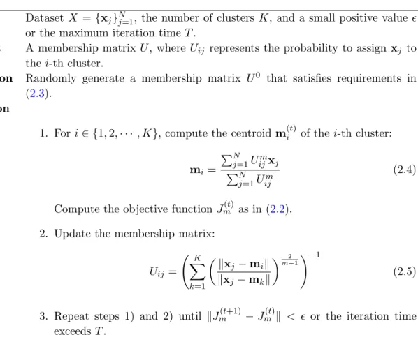
The relationship between PCA and the K-means method can also be seen when one considers the subspace spanned by the centroids. For the given dataset X that partitioned into K clusters with mk as the centroid of the k-th cluster, the between-cluster scatter matrix Sb = PK
k=1nkmkmTk can be considered as an operator that projects any vectorxinto the subspace
spanned by the K centroids. That is,
SbTx=
K X
k=1
nkmk(mTkx)
This subspace is called cluster centroid subspace in Cleuziou (2008) and the following theorem reveals its connection to the PCA dimension reduction:
Theorem 2. Cluster centroid subspace is spanned by the first K−1principal directions of the centered datasetY. The principal directionsuk (k= 1,2,· · · , K−1) are those vectors obtained from the singular value decomposition of Y and they satisfy
Y YTuk =λkuk
Proof. Consider the centered datasetY. The centroid of thek-th clusterCkcan be represented
using the cluster indicator vectorhk:
mk= P yi∈Ckyi nk =n−k1/2X i hk(i)yi=n −1/2 k Y hk
Then the between-cluster scatter matrix becomes Sb= K X k=1 Y hkhTkYT =Y K X k=1 hkhTk ! YT =Y K X k=1 qkqkT ! YT
By Theorem1,q1,· · ·, qK−1are linear transformations ofv1,· · ·, vK−1, andqK ise/N1/2. Thus K X k=1 qkqTk =eeT/N + K−1 X k=1 vkvkT
Notice that Ye= 0. By (2.6), we haveYvk=λ1/2k uk, which completes the proof.
This theorem support the effectiveness of PCA as a preprocessor of clustering methods
2.4 Extensions and Variants of K-Means Method
2.4.1 Kernel Based Fuzzy Clustering with Spatial Constraints
Among the applications of data clustering, the problem of color segmentation of a given image is one that requires clustering the pixels of the digital image based on their colors. Fig.
2.2shows the color segmentation results by applying fuzzy c-means method on a digital image with specified number of clusters as three, four, five and six respectively.
(a) Original image (b) 3 clusters (c) 4 clusters (d) 5 clusters (e) 6 clusters
Figure 2.2: (a) The original image, (b-e) Color segmentation results by applying fuzzy c-means method. In each result, the assignments of pixels are based on their maximum membership values. The number of clusters in the results are required to be K = 3, K = 4, K = 5, and K = 6 respectively.
Although the K-means method and fuzzy c-means method have been applied with empir-ical success in solving color segmentation problems, their performance are not reliable when the images are corrupted with noise or when there exists irreducible intensity inhomogeneity properties that are induced from the methods of collecting the images, for example, the radio-frequency coil in magnetic resonance imaging (MRI) Zhang et al. (2003). To avoid the case
where the color of a single pixel can affect its assignment in the clustering result dramatically, especially when considering that this pixel may be the noise of a image, methods that take into account of spatial information have been developed under the framework of the fuzzy c-means method Ahmed et al. (2002) Liew et al. (2000) qiang Zhang and can Chen (2004), where Ahmed et al. (2002) qiang Zhang and can Chen (2004) modified the objective function of the fuzzy c-means method directly to incorporate the spatial influence. At the same time, more sophisticated measures of distance can be applied in solving color segmentation problems instead of being restricted to the Euclidean distance which behave poorly when we consider clustering a complex nonlinear dataset that resides on a lower dimensional manifold embedded in a high dimensional Euclidean space. Here we discuss an image segmentation method that is proposed in Zhang et al. (2003). This algorithm is developed under the framework of the fuzzy c-means method, it incorporates the spatial information via additional constraints in the ob-jective function and uses the kernel method to represent the similarity measures between pixels.
First of all, we introduce and discuss the kernel method. Let the original dataset be X = {x}N
j=1. Instead of working directly from the given data representation as in many
other algorithms, the kernel methods try to discover more intricate information carried by the dataset by mapping it to some Hilbert space H that is called the feature space. Let the map-ping be f,f :X →H. The mapping f between the original dataset and H should benefit the comparisons for similarity measures between the original data points. Some direct examples of such mappings are functions of the components of data points (for examples, see (2.20) (2.21) (2.22) (2.23)). The similarity comparison between any pair of the mapped data points f(xi), f(xj) in the Hilbert space H is then calculated in terms of their inner product in the Hilbert space hf(xi),f(xj)i . Thus the similarity comparison between xi and xj is defined as the one
betweenf(xi) and f(xj), and finally represented in terms of the inner product in H. In other
words, the inner products of the mapped data points are able to define the similarity measures between the original data points. Hence, in order to compare data points in terms of their similarities, it is unnecessary to know the explicit mapping f from the original dataset to the feature space if we can define the inner products in the feature space.
Now, let us represent the inner products of any pairs of data points in the format of a function,k:X×X→R, wherek(xi,xj) =hf(xi),f(xj)i. The functionk is called a kernel. It
is important to notice that not all functions can be interpreted as the inner product function of its inputs. The following theorem Jean-Philippe Vert and Scholkopf (2004) give a detailed description of a kernel:
Theorem 3. If a functionkis symmetric and positive semi-definite, then it can be interpreted as the inner product of the mapped data points in the feature space and it is called a positive definite kernel.
Here, k is symmetric means k(xi,xj) =k(xj,xi), for any two data points xi,xj. And k is
positive semi-definite means:
n X i=1 n X j=1 aiajk(xi,xj)≥0
for anyn >0, any choices ofx1,x2,· · · ,xn∈Xand any choices of real numbersa1, a2,· · · , an∈
R.
Some simple examples of kernels include (1). Gaussian radial basis function (RBF) kernel:
kG(x,x0) = exp −d(x,x 0)2 2σ2 (2.20) (2). Linear kernel: k(x,x0) =x>x0 (2.21) (3). Polynomial kernels: kpoly1(x,x0) = (x>x0)d (2.22) or kpoly2(x,x0) = (c+x>x0)d (2.23)
More kernels can be generated through operations upon existing kernels or learned from the given datasets (see section 1.6 and 1.7 inJean-Philippe Vert and Scholkopf (2004)).
After the kernel to be used in a clustering algorithm is chosen, every inner product in the feature space can be replaced by the kernel expression. This is the so-called kernel trick. Many clustering algorithms that only use the inner products of data points have been improved with the kernel trick by replacing the inner products of the original data points with the related kernel function values Hoffmann (2007) qiang Zhang and can Chen (2004) Jean-Philippe Vert and Scholkopf (2004). The kernel trick enables the application of clustering algorithm on the mapped dataset f(X) in the feature space H without knowing the explicit mapping f. One of the most popular kernel methods is Supported Vector Machine (SVM) (see section 1.4 in Jean-Philippe Vert and Scholkopf (2004)).
Now we are ready to discuss a kernelized fuzzy c-means algorithm with spatial constraints qiang Zhang and can Chen (2004).
To cluster a given datasetX ={xj}N
j=1 intoK clusters, the fuzzy c-means method aims at
minimizing the objective function
Jm= K X i=1 N X j=1 Uijm||xj −mi||2
Where membership matrix U = (Uij) satisfies
0≤Uij ≤1, ∀i, j and K X
i=1
Uij = 1, ∀j= 1,2,· · · , N
Since the objective function under minimization only uses the Euclidean distance that can be rewritten as the inner productshxj−mi,xj−mii for alli, j, it is suitable to replace the inner
product in Euclidean space with the inner product in the feature spaceH by incorporating the kernel trick. So, we can derive the kernelized fuzzy c-means method by applying fuzzy c-means method in the feature space H. The resulting objective function is:
Jm= K X i=1 N X j=1 Uijm||f(xj)−f(mi)||2
Notice that
kf(xj)−f(mi)k2 =hf(xj)−f(mi),f(xj)−f(mi)i
=hf(xj),f(xj)i − hf(mi),f(xj)i − hf(xj),f(mi)i+hf(mi),f(mi)i
=k(xj,xj) +k(mi,mi)−2k(xj,mi)
If one uses the Gaussian kernel as defined in (2.20) from now on, then k(x,x) = 1 for any
x, thus the objective function under minimization can be written as:
Jm = 2 K X i=1 N X j=1 Uijm(1−k(xj,mi)) (2.24)
The constraints used in qiang Zhang and can Chen (2004) are the following:
0≤Uij ≤1, K X i=1 Uij = 1,∀j, and 0< N X j=1 Uij < N, ∀i (2.25)
Following the similar method in minimizing the objective function in fuzzy c-means method, the local minima of Jm for the kernel fuzzy c-means method can be found as:
Uij =
(1−k(xj,mi))−1/(m−1) PK
k=1(1−k(xj,mk))−1/(m−1)
(2.26)
and the centroid of thei-th cluster can be found as:
mi = PN k=1Uikmk(xk,mi)xk PN k=1Uikmk(xk,mi) (2.27)
Since the performance of segmentation algorithms can be affected if the image is corrupted by noise, spatial information or constraints can be taken into consideration in designing meth-ods that are able to filter noise. On top of such kernelization of the standard fuzzy c-means method, qiang Zhang and can Chen (2004) introduced a spatially constrained term in the objec-tive function to bias the segmentation toward piecewise-homogeneous labeling. The improved objective function requires that for any fixed data point that, for example, is more likely to be clustered in the ith cluster, its neighboring data points should also be more likely to be assigned to the same cluster. To express this idea mathematically, and take into consideration of all the possible assignments of each data point that is weighted by its membership values, the objective function improved with spatial constraints is defined as the following:
Jm= K X i=1 N X j=1 Uijm(1−k(xj,mi)) + α NR K X i=1 N X j=1 Uijm X r∈Nj (1−Uir)m (2.28)
With constraints as in (2.25). HereNj is the set of neighbors in a window aroundxj,NRis the
cardinality of Nj. α controls the effect of the spatial penalty term and it is set to be between
zero and one.
Similarly, the formulas for calculating membership matrix U and the set of centroids can be derived by using Lagrange multipliers. For a given set of centroids, the membership values can be updated to Uij = 1−k(xj,mi) +αP r∈Nj(1−Uir) m/N R −1/(m−1) PK k=1 1−k(xj,mk) +α P r∈Nj(1−Ukr) m/N R −1/(m−1) (2.29)
Since the spatial constrain is not related to any of the centroids {mi}K
i=1, then for a given
membership matrixU, the calculation for centroids are the same as in (2.27).
Finally, the process to find local minima (as candidates for the global minimization) of the objective function can be summarized in Table2.3.
The added spatial constraints can effectively reduce the effects of noise in the clustering results. Fig. 2.3compares the segmentation results on an magnetic resonance image by fuzzy c-means method and the kernel based fuzzy clustering method with spatial constraints (SKFCM) described above. The original image is from the U. S. National Library of Medicine, and it is then corrupted by Gaussian noise with mean 0 and variance 0.0009. Kernel used for the results is the Gaussian radial basis function kernel as in (2.20) withd(·,·) being the Euclidean distance and 2σ2= 0.15. The parameterα is set to be 0.15 and the number of neighbors in the window around every data point is NR = 8. That is, all data points inside a 3 by 3 window centered
at a fixed data pointxare considered as its neighbors except the data point xitself. After the initiation by generating a random membership matrix U, the first iteration calculate the set of centroids by using (2.4). After that the calculations follow the procedures described in the algorithm of SKFCM.
Table 2.3: Image segmentation by the kernel-based fuzzy c-means method with spatial con-straints (SKFCM)
Step 0: Choose a kernel ksuch that k(x,x0) is the inner product of the images of x and
x0 in the feature space. In the current discussion, kis chosen to be the Gaussian radial basis function (RBF) kernel:
kG(x,x0) = exp −d(x,x 0)2 2σ2
Step 1: Initialize the membership matrixU satisfying the constraints as in (2.25).
Step 2: For timet= 1,2,· · ·, tmax, do the following iteration:
1. base on the current membership values, compute all centroids according to (2.27).
2. base on the updated centroids, compute all membership values according to (2.29).
3. let the maximum of the updates in membership values beerrt= max
i,j|Uijt−
Uijt−1|. Iferrt≤, stop.
(a) (b) (c)
Figure 2.3: Results of segmentation on a magnetic resonance image corrupted by Gaussian noise with mean 0 and variance 0.0009. (a). The corrupted image. (b). Segmentation result obtained by applying fuzzy c-means method with 5 clusters. (c). Segmentation result obtained by applying SKFCM with 5 clusters. The parameters that used to obtain the results can be found in the text.
2.4.2 The Extension of K-means Method for Overlapping Clustering
Among various methodologies developed to solve clustering problems for large amount of data that are heterogeneous in nature, overlapping clustering arises as one that aims at or-ganizing the dataset into a collection of clusters such that every data point is assigned to at least one cluster and the union of the collection of clusters is the original dataset. Overlapping clustering has some unique properties. It allows different clusters overlapping with each other while crisp clustering does not, and its result only indicates the assignments of each data point to multiple clusters without generating membership values as fuzzy clustering does. These characteristics of overlapping clustering are beneficial in clustering data points which have at-tributes that can be categorized differently based on multiple perspectives. The applications of overlapping clustering can be recognized in solving various practical problems. For example, information retrieval requires documents to be clustered by domains and each document has multiple domains. Also, in bioinformatics it is likely that the genes to be clustered contribute to multiple metabolic pathwaysCleuziou (2008) Cleuziou (2010).
Different methodologies have been developed through the last four decades for overlapping clustering. Some earlier approaches can be found in Dattola (1968) Jardine and Sibson (1971) Diday (1987). Some more recently research extends existing partition clustering methods to overlapping clustering. For example, the Model-based Overlapping Clustering (MOC) Baner-jee et al. (2005a) extends the CEM method proposed in Celleux and Govaert (1992). Also, an extended version of the K-means method, overlapping K-means method (OKM), is proposed in Cleuziou (2008) for overlapping clustering. This section focuses on the description of OKM method proposed in Cleuziou (2008).
For a given dataset X = {xi}Ni=1 ⊂ Rp and a given number of clusters k, OKM aims
at minimizing the total distance between data points and their “images” represented by the prototypes of clusters, where the prototypes are the centroids of the clusters. If we denote the clusters as {πi}ki=1, and the centroids as {mi}ki=1, then the goal of OKM is to minimize the
following objective function:
J({πi}ki=1) = X
xi∈X
kxi−φ(xi)k2 (2.30)
whereφ(xi) is the “image” ofxidenoted by prototypes, i.e. ifxi is assigned to multiple clusters
and Ai ={mc|xi∈πc} is the set of centroids of the related clusters, thenφ(xi) is defined by
φ(xi) = P
mc∈Aimc |Ai|
(2.31)
and |Ai|is the number of elements in the setAi.
It is clear to see that the above objective function is a generalization of the one used in the K-means method since the former reduces to the latter when we require that each data point is assigned to only one cluster.
The algorithm that realizes the above minimization of objective function is an iterative pro-cedure that alternates between calculating the centroids of clusters and assigning data points to multiple clusters with the initiation of the algorithm as a random selection of the set of centroids {πi(0)}k
i=1. The two alternative procedures are described as follows.
When given the set of centroids {mi}ki=1, the assignment of each data point to multiple
clusters is not a trivial task because there exists 2k choices of such multiple assignments for each data point theoretically. Thus a heuristic method is employed such that the assignment of each data point first favors the clusters whose centroids are closest to the data point, and the assignments to clusters are made if the resulting image of the data point is improved in terms of minimizing the objective function. The procedure of assigning a data point xi to multiple
clusters is described in Table2.4.
Then, the problem of calculating the centroidmh of a given clusterπh based on the
assign-ments of data points to multiple clusters and thek−1 centroids{mi}ki=1\ {mh}that minimizes
Table 2.4: Multiple Assignment of A Data Point
Input: A data point xi, the set of centroids{mi}ki=1, and the set of centroids Aoldi that
corresponds to the assignment of xi in the previous iteration step. Output: Ai, a set of the centroids that defines the multi-assignment forxi.
1. Let Ai ={m∗} such thatm∗ = arg min{mi}ki=1kxi−mik
2. Computeφ(x i)
with the current Ai.
2. Find the nearest centroid: m0 = arg min{mi}k
i=1\Aikxi−mik
2. Compute
the image φ0(xi) withAiS{m0}.
3. Ifkxi−φ0(xi)k<kxi−φ(xi)k, letm0be contained in Ai, setφ(xi) =φ0(xi)
and go to step 2; Otherwise compute φold(xi) withAoldi . If kxi−φ(xi)k ≤ kxi−φold(xi)k, output Ai, else output Aoldi .
calculation ofmh is as the following:
mh = 1 P xi∈πhαi X xi∈πh αimih (2.32)
whereαi= 1/|Ai|2 denotes the sharing ofxi among clusters, andmih can be considered as the
ideal centroid that matchesxi with its imageφ(xi):
mih =|Ai| ·xi−
X
mc∈Ai\{mh}
mc
Table 2.5: OKM Algorithm
Input: A dataset X ={xi}ki=1, the number of clusters k. Optional maximum number
of iterations tmax, optional threshold on the objective. Output: {πi}ki=1 as the final coverage of the dataset.
1. Draw randomlyk points inRp or X as the initial centroids{m(0)i }ki=1.
2. For eachxi ∈Xcalculate the assignmentA(0)i to derive the initial coverage {π(0)i }k
i=1.
3. Sett= 0.
4. For each clusterπ(t)i successively compute the new centroid as in (2.32).
5. For each xi ∈ X compute the assignment A(t+1)i as described above and
then derive the coverage {πi(t+1)}k i=1.
6. If not converged or t < tmax orJ({π(t)})−J({π(t+1)})> , set t =t+ 1
and go to step 4. Otherwise, stop and output the final clusters{π(t+1)i }k i=1.
CHAPTER 3. Spectral Clustering Methods
3.1 Introduction
Spectral clustering has become one of the most important clustering methods over the past decade. The theoretical developments of spectral clustering methods viewed from different as-pects have led to successful applications in broad areas of study including color segmentation, protein classification, face recognition, collaborative recommendation and so on Meila and Shi (2000) Cour et al. (2005a) Cour and Shi (2004) Cour et al. (2005b) Enright et al. (2002) Pac-canaro et al. (2003). The popularity of spectral clustering are due to but not limited to its profound theoretical supports, convenient implementation, and rich mathematical outreach.
Some standard clustering methods, for example, the K-Means method, usually fail in the case where the datasets reside on nonlinear manifolds that are embedded in higher dimensional spaces. The reason lies in the fact that, these methods like the K-Means method utilize the Euclidean distances in the space occupied by the data points instead of the metric of the under-lying manifold. Spectral methods are able to handle complex nonlinear datasets by detecting the intricate data structure, which will be discussed in the following sections. The implemen-tation of the spectral clustering turns out to be easy, and the compuimplemen-tational complexity boils down to the calculations of first few eigenvectors of (sparse) matrices Shi and Malik (2000) Luxburg (2007).
Several slightly different versions of spectral clustering methods have been derived in dif-ferent theoretical background including graph partition Shi and Malik (2000), perturbation theory Stewart and Sun (1990) Luxburg (2007), and stochastic processes on graphs Meila and
Shi (2000) Fouss et al. (2006). The main operator involved in the spectral clustering, the graph Laplacian, can also be seen as a discrete analogy of the Laplace-Beltrami operator under appropriate conditions Singer (2006) Rosenberg (1997) Belkin and Niyogi (2005). Extended studies of spectral clustering give rise to mechanics targeting more specific applications, and efforts have been made to derive variational methods based on spectral clustering Cour and Shi (2004) Bach and Jordan (2004) Cour et al. (2005a).
The outreach of spectral clustering includes its connections to kernel methods and to clus-tering methods based on random walks. Such connections provide insights into the related mechanisms and allow possible adaptations between these clustering methods Gutman and Xiao (2004) Bie et al. (2006).
Although spectral clustering has advantages as mentioned above, its performance still relies on several factors, for example, how to measure the distances between data points, and how to decide the number of clusters. This chapter is devoted to the review on the spectral clustering methods. The rest of this chapter is arranged as follows: section 2 summarizes the derivation and algorithms of spectral clustering methods, focusing on the connections between spectral clustering and several other related topics including the graph cut problem, random walks on the graph, perturbation theory, and Laplace-Beltrami operator. Section 3 describes some applications of spectral clustering in the fields of image segmentation and shape recognition. Section 4 discusses some techniques that can be used to refine the spectral clustering.
3.2 The Derivations and Algorithms of Spectral Clustering Methods
Spectral clustering methods have been derived under various mathematical settings, and the corresponding algorithms can be classified as unnormalized spectral clustering or normalized spectral clustering. The current section is devoted to the derivations of spectral clustering methods and the descriptions of related algorithms.
3.2.1 Graph Cut and Spectral Clustering
Considering solving a clustering problem on a given dataset X = {xi}Ni=1, our goal is to
partition the whole dataset into k clusters C1, C2,· · ·, Ck such that data points assigned to a
same cluster are similar and data points assigned to different clusters are dissimilar. There are many possible choices of measuring the similarities between data points, and such a measure should be decided based on the specific problems. For example, the similarity measure can be defined as the inverse of the Euclidean distances between data points, or be uniform between a data point that is under consideration to its fixed number of nearest data points, etc. A graphG= (V, E) can be constructed to represent data points and show how similar any pairs of data points are. That is, we can take the set of graph nodes V as the dataset X and E as the set of edges between any pairs of nodes in V. Then we can define the weight wij on
the edge which links xi and xj as the similarity measure between them. The weight matrix
W is anN byN matrix that represents all weights on edges and it is denoted asW = (wij)N×N.
Thus the goal of data clustering on dataset X can be considered as cutting (partitioning) the graph G into k non-overlapping groups such that the weights on inner group edges are high while the weights on intergroup edges are low. To achieve a reasonably good graph cut, measures on the quality of the graph cut should be designed accordingly.
An intuitive measuring method is derived by considering the total similarity between any pairs of different groups. That is, a better graph cut is characterized by a smaller total similarity. If we denote Cic as the complement of Ci, then the similarity between a group Ci with any
other groups {Cj}j6=i are calculated as
W(Ci, Cic) = X
u∈Ci,v∈Cic
wuv (3.1)
Thus, the total similarity between any pairs of different groups can be calculated as the following and it is called thecut in graph theoretical language.
cut(C1, C2,· · ·, Ck) = 1 2 k X i=1 W(Ci, Cic) (3.2)
Here, the factor 1/2 is introduced such that every intergroup edge is considered only once. An algorithm that minimizes the cut defined above will result in a partition that allows small similarities between different clusters. For k = 2, the problem of finding the minimum cut is well studied and Stoer and Wagner (1997) gives an efficient algorithm.
However, as pointed out in Wu and Leahy (2002) and Shi and Malik (2000), the partition generated by minimizing the cut tends to have small clusters of isolated data points only be-cause such isolated data points have much lower similarities to any other data points compared to the rest of the dataset. Such clustering results do not provide any further insights on the data structure other than separating out several isolated data points. It is clear that the measure
cut only takes into account the intergroup similarities and it often fails to serve as a quality measure of the clustering result for general datasets. Two different measures of the clustering quality that are able to circumvent this problem are discussed below. One of them leads to the normalized spectral clustering and the other leads to the unnormalized spectral clustering.
3.2.1.1 Ncut
Shi and Malik proposed a quality measure, called normalized cut (Ncut) in Shi and Malik (2000), to circumvent the above problem. The idea is to generate “balanced” clusters whose total similarities to the rest of the dataset are small after normalized by their inner-cluster similarities. LetV be the set of nodes, we consider a partition{C1, C2,· · · , Ck}ofV such that Sk
i=1Ci =V and Ci T
Cj =∅, ∀i6=j. The normalized cut of the partition {C1, C2,· · · , Ck}
is defined as the following:
N cut(C1, C2,· · · , Ck) = k X i=1 cut(Ci, Cic) assoc(Ci, V) (3.3)
where assoc(A, B) is defined as the total similarity between two groups A and B, and Ac represents the complement ofA. That is,
assoc(A, B) = X
u∈A,v∈B
To verify that the minimization of Ncut defined above provides a partition that has mini-mized intergroup similarities and ensures the results are “balanced” clusters with high inner-group similarities, Shi and Malik (2000) considers the normalized association within inner-groups:
N assoc(C1, C2,· · ·, Ck) = k X i=1 assoc(Ci, Ci) assoc(Ci, V) (3.5)
Thus, a maximized Nassoc indicates that the groups in the partition {C1, C2,· · · , Ck} have
high within group similarities compared to their total similarities to the whole dataset. The relationship betweenNassoc and Ncut is shown by the following:
Proposition 4. N cut(C1, C2,· · · , Ck) =k−N assoc(C1, C2,· · · , Ck) (3.6) Proof. N cut(C1, C2,· · ·, Ck) = k X i=1 cut(Ci, Cic) assoc(Ci, V) = k X i=1 assoc(Ci, V)−assoc(Ci, Ci) assoc(Ci, V) = k X i=1 1−assoc(Ci, Ci) assoc(Ci, V) =k− k X i=1 assoc(Ci, Ci) assoc(Ci, V) =k−N assoc(C1, C2,· · ·, Ck)
Thus, the minimization ofNcut also means the maximization of Nassoc. Thus it is reason-able to considerNcut an appropriate measure on the quality of a clustering result. Algorithms that minimize Ncut are capable of maximizing the within group similarities and minimizing the intergroup similarities simultaneously. Although Ncut provides a better quality measure on the clustering results, the exact minimization ofNcut is NP-complete Shi and Malik (2000).
To solve the problem, calculations in Shi and Malik (2000) showed thatNcut can be rewrit-ten in the form of a Rayleigh quotientGolub and Van Loan (1989) using a type of matrix called graph Laplacian Chung (1997), which will be introduced below. A type of spectral cluster-ing method was designed based on a relaxation of the minimization of this Rayleigh quotient. Shi and Malik (2000) gives details of this derivation, here we follow the procedure provided in Luxburg (2007) for a simplified version to show the relationship between Ncut and graph Laplacian.
First, we introduce some notations and discuss some properties of graph Laplacian. More discussions can be found in the book by Chung Chung (1997). Given the weight matrix W, one can define the degree at each nodexi asdi=PNj=1wij. The degree matrixDis defined as
D=diag(d1, d2,· · ·, dN) (3.7)
The graph Laplacian is defined as
L=D−W (3.8)
Some properties of the graph Laplacian can be summarized by the following
Proposition 5. For a given non-negative symmetric weight matrix W = (wij)N×N, the graph Laplacian L is symmetric and positive semi-definite. L has N non-negative eigenvalues λ1 ≤
λ2 ≤ · · · ≤λN and the corresponding eigenvectors v1, v2,· · · , vN are orthogonal to each other. The smallest eigenvalue is λ1= 0 and the corresponding eigenvector is 1= (1,1,· · · ,1)T.
Proof. SinceDis a diagonal matrix, it is clear thatL=D−W is symmetric ifW is symmetric. Then L has N eigenvalues {λi}Ni=1 and the corresponding eigenvectors are orthogonal to each
other.
The eigenvectors of L provide information of the number of connected components of the graphG Mohar (1991)Mohar and Juvan (1997).
Proposition 6. The multiplicity n of the eigenvalue 0 of L equals the number of connected components A1,· · · , An in the graph G. The eigenspace of eigenvalue 0 is spanned by the indicator vectors 1A1,· · · ,1An.
Next, for any arbitrary vector yinRN,
2yTLy= 2(yTDy−yTWy) = N X i=1 diyi2−2 N X i,j=1 wijyiyj+ N X j=1 djyj2 = N X i=1 N X j=1 wijy2i −2 N X i,j=1 wijyiyj + N X j=1 N X i=1 wijyj2 = N X i,j=1 wij(yi−yj)2
Since W is non-negative, yTLy ≥ 0 for any arbitrary vector y in RN. That is, L is positive
semi-definite. Thus, all eigenvalues ofLare non-negative and it is easy to see that the smallest eigenvalue is 0 corresponding to an eigenvector1= (1,1,· · ·,1)T.
We now consider the case of bipartition of the graph (k = 2). The analogical conclusions in cases where k≥2 can be derived similarly Luxburg (2007).
Now consider the bipartition (the case where k=2) of a graph Gusing Ncut as the quality measure (the cases where k ≥ 3 will be discussed later). For a bipartition {C1, C2} of the
set of nodes V (C1 ∪C2 = V and C1 ∩C2 = ∅) one can define the indicator vector as f =
(f1, f2,· · · , fN)T such that f carries the bipartition information. That is, fj = afor xj ∈C1
and fj =b forxj ∈C2, where a, bare two different constants. If one chooses to define f as
fi = q vol(C2) vol(C1) ifxi ∈C1 −qvol(C1) vol(C2) ifxi ∈C2 (3.9)
relationship between graph Laplacian andNcut, here we usei∈Cj to representxi ∈Cj,∀i, j: 2fTLf = N X i,j=1 wij(fi−fj)2 = X i∈C1,j∈C2 wij s vol(C2) vol(C1) + s vol(C1) vol(C2) !2 + X i∈C2,j∈C1 wij − s vol(C1) vol(C2) − s vol(C2) vol(C1) !2 = X i∈C1,j∈C2 wij vol(C2) vol(C1) +vol(C1) vol(C2) + 2 + X i∈C2,j∈C1 wij vol(C1) vol(C2) +vol(C2) vol(C1) + 2 = 2 vol(C1) vol(C2) + vol(C2) vol(C1) + 2 cut(C1, C2) = 2 vol(C1) +vol(C2) vol(C2) +vol(C1) +vol(C2) vol(C1) cut(C1, C2) = 2vol(V)N cut(C1, C2) That is , fTLf =vol(V)N cut(C1, C2) (3.10)
Also one can check that (Df)T1= 0 andfTDf =vol(V). Then by allowingf to be an arbitrary vector inRN, one can derive a relaxation of the minimization ofNcut.
min
f∈RN
fTLf subject to Df ⊥1, fTDf =vol(V) (3.11)
Now we can introduce the following substitution g=D1/2f and the above problem can be rewritten as
gTD−1/2LD−1/2g
subject to g⊥D1/21, ||g||2 =vol(V) (3.12)
D−1/2LD−1/2 is symmetric and it is a version of normalized graph Laplacian. It can be denoted as
Lsym=D−1/2LD−1/2 (3.13)
A similar calculation reveals that for arbitraryy∈RN,
yTLsymy= N X i,j=1 wij yi √ di −pyj dj !2
Thus, Lsym is positive semi-definite. Use the fact that it is symmetric, we can conclude that
Lsym has N non-negative eigenvalues {λi}Ni=1 with eigenvectors {vi}Ni=1 orthogonal to each
other. Also, the smallest eigenvalue is λ1 = 0 with at least one corresponding eigenvector v1 =D1/21.
Similar to Proposition 6,Lsym has properties described as follows:
Proposition 7. The multiplicityn of the eigenvalue0of Lsym equals the number of connected components A1, A2,· · · , An in the graph G. The eigenspace of eigenvalue 0 is spanned by the indicator vectors D1/21 A1, D 1/21 A2,· · · , D 1/21 An.
Considering the above properties of Lsym, the minimization in (3.12) can be transformed
to the standard form of the Rayleigh quotientGolub and Van Loan (1989) in finding g1 such
that: g1= arg min gTg 0=0 gTD−1/2LD−1/2g gTg (3.14) whereg0=D1/21.
Notice that in the current setting we assume that similarity measures of any pairs of nodes are nonzero, thus the graph G is complete. By Proposition 7, D1/21 is the only eigenvector that corresponds to eigenvalue 0. Thus the solution is parallel to the eigenvector of Lsym that
corresponds to the smallest positive eigenvalue. Also, the above is equivalent to findingf1such
that:
f1 = arg min fTD1
fT(D−W)f
fTDf (3.15)
Then this problem can be solved by finding the eigenvector f corresponds to the smallest positive eigenvalue of the generalized eigenvalue problem:
Lf =λDf (3.16)
The solution f1 serves as an indicator vector for the bipartition ofV. As mentioned before, in
the cases where the number of clusters k > 2 the above procedure holds due to similar argu-ments. Then the partition of components of f1 corresponds to the optimized partition of V.