Institut für Nutzpflanzenwissenschaften und Ressourcenschutz Professur für Pflanzenzüchtung
Prof. Dr. J. Léon
Bayesian Adaptive Markov Chain Monte Carlo Estimation of Genetic Parameters
Inaugural-Dissertation zur
Erlangung des Grades Doktor der Agrarwissenschaften
(Dr. agr.)
der
Hohen Landwirtschaftlichen Fakultät der
Rheinischen Friedrich-Wilhelms-Universität Bonn Zu Bonn vorgelegt am 08-12-11 von Boby Mathew aus Kottayam, Indien
Referent: Prof. Dr. Jens Léon Korreferent: Prof. Dr. Heiko Schoof Tag der mündlichen Prüfung: 23-03-12
ACKNOWLEDGMENTS
Acknowledgments
First and foremost, my utmost gratitude to my supervisor, Prof. Dr. Jens L´eon for his encouragement, patience, motivation, enthusiasm, immense knowledge and continuous support throughout my PhD study. I consider it an honor to work with him and he has been my inspiration in the completion of this research work. I owe my deepest gratitude to Prof. Dr. Jens L´eon for his excellent supervision.
I also express my deepest gratitude to Dr. Andrea Bauer for her guidance, kind support, valuable suggestions and discussions, that laid the foundations for my PhD Work.
Also I would like to express my sincere gratitude to Dr. Mikko J. Sillanp¨a¨a and Dr. Petri Koistinen, university of Helsinki for their guidance and valuable suggestions throughout my research study.
Meanwhile I am grateful to Dr. H. Schumann and Mrs Anne Reinders for their technical guidance. Also I would like to thank Dr. A. Ballvora and Dr. A. Naz for the scientific discussions. I offer thanks to Mrs Annette Schneider who helped me to have a nice working atmosphere.
Special thanks to Ana for the valuable suggestions and comments which helped me to improve my thesis. Also I would like to thank Hedda von Quistorp and Karin Woitol for their technical assistance. I am grateful to my colleagues Bong-Song, Tigest, Ismail, Ranya, Mohammed, Wiebke, Melanie, Alexendra, Merle and Karola for their mutual support and friendly working atmosphere. Many thanks to my Indian friends for their kind support. For the financial support I am thankful to the Theodor-Brinkman-Graduate School of the Faculty of Agriculture at the University of Bonn.
Finally my deepest gratitude to my beloved parents, my brother and sister for their love, support and encouragement throughout my study.
LIST OF TABLES AND FIGURES
List of Tables
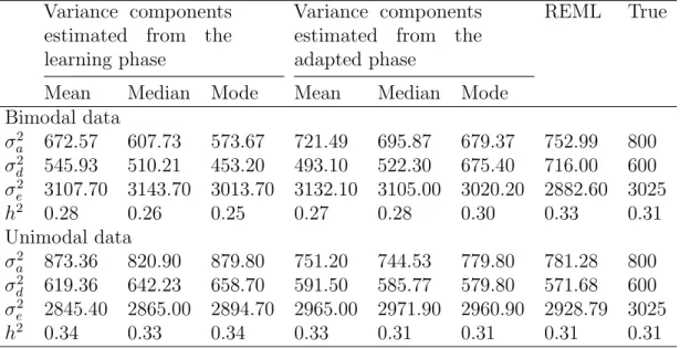
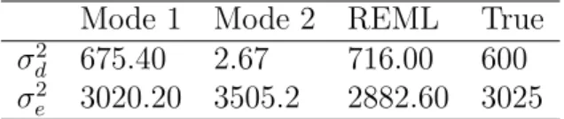
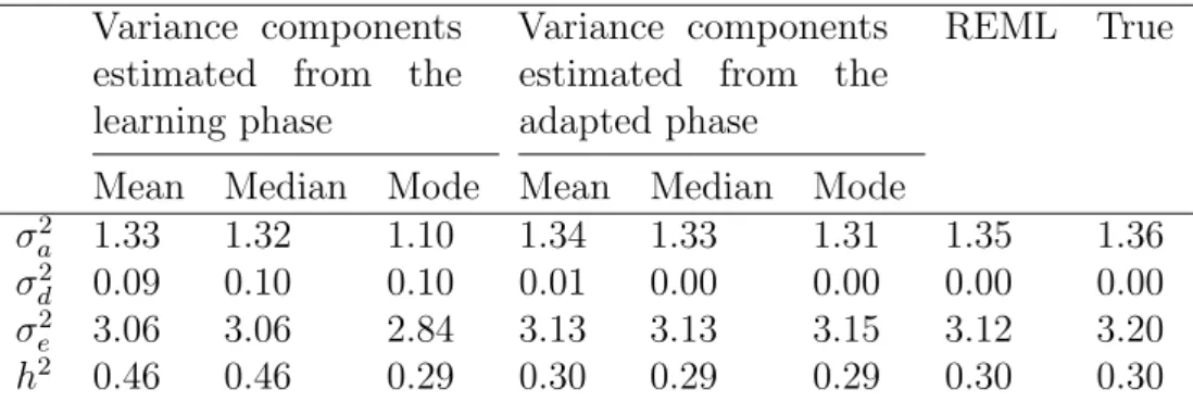
Table 1: The estimates of variance components and broad-sense heritabilities for the learning and adapted phases from the MCMC analyses of the two simu-lated datasets...57 Table 2: The two different modes of the variance components for the simulated bimodal dataset...62 Table 3: The estimates of the variance components and broad-sense heritabil-ities for the learning and adapted phases from the MCMC analysis of the QTL-MAS XII dataset...63 Table 4: Effective Sample size (ESS) for 3000 iterations of the two MCMC algo-rithms with the unimodal, bimodal and QTLMAS datasets...65 Table 5: Effective Sample Size (ESS) for 3000 iterations from the learning phase and 3000 iterations from the adapted phase for the class 2 MCMC with the unimodal, bimodal and QTLMAS datasets...66 Table 6: The estimates of the variance components and broad-sense heritabil-ities for the learning and adapted phases from the class 2 algorithm of the QTLMAS XII dataset...66 Table 7: Effective Sample size(ESS) for the Scaled inverse chi-square prior and Gamma prior distribution for the workshop data...69 Table 8: The variance components and broad-sense heritability for different prior distributions for the bimodal, unimodal and workshop datasets...73 Table 9: The variance components and broad-sense heritability for different prior distributions for the workshop data...73 Table 10: The estimates of the variance components and broad-sense heri-tabilities for the learning and adapted phases from the MCMC analysis of the QTLMAS XII dataset using two different prior distributions in the learning phase...75
LIST OF TABLES AND FIGURES
Table 11: Effective Sample size (ESS) for 3000 iterations from the learning phase and 45000 iterations from the adaptive phase of the MCMC algorithm us-ing different priors in the learnus-ing phase with QTLMAS dataset...76 Table 12: The estimates of the variance components and broad-sense heri-tabilities for the learning and adapted phases from the MCMC analysis of the simulated dataset with finite number of loci...78 Table 13: Effective Sample size (ESS) for 3000 iterations from the learning phase and adapted phase for the simulated dataset with finite number of loci...78 Table 14: Correlation coefficient (r) calculated between the estimated breed-ing value and the true genetic value usbreed-ing REML and adaptive MCMC method...80 Table 15: The estimates of variance components, heritabilities and the 95% HPD intervals for the field data from the adapted phases of the algorithm using Bayes ID and Bayes Aextcovariances...81
List of Figures
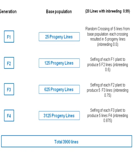
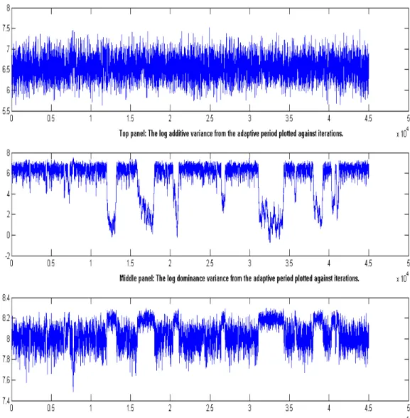
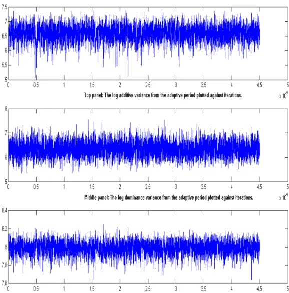
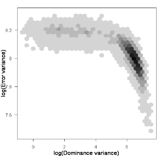
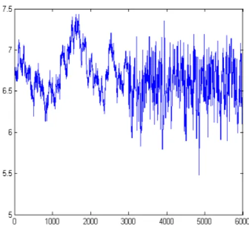
Figure 1: Schematic representation of the crossing of simulated dataset with finite number of loci till F4 generations...55 Figure 2: The logarithm of the variance components for the bimodal dataset plotted against MCMC iteration number...58 Figure 3: The logarithm of the variance components for the unimodal dataset plotted against MCMC iteration number...59 Figure 4: Histogram of the log-transformed dominance and error variance components using hexagonal bins...61
LIST OF TABLES AND FIGURES
Figure 5: Trace plot of the log-transformed additive variance component for the unimodal simulated dataset...64 Figure 6: The logarithm of the variance components for the workshop dataset with scaled inverse chi-square prior plotted against MCMC iteration num-ber...67 Figure 7: The logarithm of the variance components for the workshop dataset plotted against MCMC iteration number...68 Figure 8: The logarithm of the variance components for the bimodal dataset with scaled inverse chi-square prior plotted against MCMC iteration num-ber...70 Figure 9: The logarithm of the variance components for the bimodal dataset with Gamma prior plotted against MCMC iteration number...71 Figure 10: Trace plot of the log-transformed variance component for the simu-lated dataset with finite number of loci from the adapted phase of the class 1 adaptive MCMC algorithm...77
ABBREVIATIONS
Abbreviations
Abbreviation Explanation BV Breeding Value
BLUP Best Linear Unbiased Prediction ESS Effective Sample Size
MCMC Markov Chain Monte Carlo ML Maximum Likelihood M-H Metropolis–Hastings
MVN Multivariate Normal Distribution REML Restricted Maximum Likelihood
TABLE OF CONTENTS
Zusammenfassung 9
Abstract 11
1 Introduction 12
1.1 Phenotype and Genotype . . . 12
1.1.1 Phenotypic variation . . . 12
1.2 Breeding Value (BV) . . . 14
1.3 Inbreeding . . . 16
1.4 Heritability . . . 16
1.5 Statistical Modeling . . . 17
1.6 Restricted Maximum Likelihood (REML) method . . . 18
1.7 Bayesian Methods . . . 19
1.8 Prior Distributions . . . 21
1.8.1 Non informative priors . . . 21
1.8.2 Informative priors . . . 21
1.9 Markov Chain . . . 21
1.10 Markov Chain Monte Carlo (MCMC) . . . 22
1.11 Mixing . . . 23
1.12 Identifiability Problem . . . 23
1.13 Objectives . . . 25
2 Models and Methods 27 2.1 Additive Relationship Matrix . . . 27
2.2 Dominance Relationship Matrix . . . 28
2.3 The Mixed Linear Model . . . 28
TABLE OF CONTENTS
2.5 The Metropolis-Hastings algorithm . . . 32
2.6 Adaptive MCMC . . . 33
2.6.1 Marginalization . . . 34
2.6.2 Hierarchical model 1 . . . 34
2.6.3 Hierarchical model 2: . . . 36
2.6.4 Estimation in the learning phase: . . . 37
2.6.5 Estimation in the adapted phase (class 1) . . . 38
2.7 Adaptive MCMC (Class 2) . . . 41
2.8 Calculation of the likelihood ratio . . . 42
2.9 Adaptive MCMC algorithm . . . 43
2.10 Chi-square prior: . . . 45
2.11 MCMC convergence diagnostics . . . 46
2.12 Effective Sample Size (ESS) . . . 46
2.13 Algorithm to calculate breeding value . . . 47
2.14 Restricted Maximum Likelihood (REML) . . . 48
2.15 QTLMAS XII workshop data . . . 50
2.16 Simulated data . . . 50
2.17 Simulated dataset with finite number of loci . . . 51
2.18 Field data: . . . 53
3 Results 56 3.1 Class 1 adaptive MCMC . . . 56
3.1.1 simulated data . . . 56
3.1.2 QTLMAS XII workshop data . . . 62
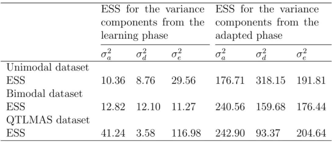
3.1.3 Effective Sample Size . . . 63
3.2 Class 2 adaptive MCMC . . . 65
TABLE OF CONTENTS
3.4 Estimation using scaled inverse chi-square prior distribution in
the learning phase . . . 74
3.5 Simulated dataset with finite number of loci . . . 76
3.6 Estimation of breeding values . . . 79
3.7 Field data . . . 80
4 Discussion 82 4.1 Computational cost (Adaptive MCMC vs hybrid Gibbs sampler) 82 4.2 Estimation of breeding values . . . 83
4.3 Inbreeding and the genetic complexity . . . 84
4.4 Estimation of Variance components . . . 85
4.5 Identifiability problem . . . 86
4.6 Importance of the optimal proposal covariance structure . . . 87
4.7 Effects of marginalization and Mixing . . . 88
4.8 Impact of Prior Distributions and sensitivity analysis . . . 90
5 Summary and Conclusion 91
ZUSAMMENFASSUNG
Zusammenfassung
Eine exakte Sch¨atzung von genetischen Parametern ist entscheidend f¨ur ein leistungsf¨ahiges genetisches Evaluierungssystem. Normalerweise werden REML- und Bayes-Verfahren f¨ur die Sch¨atzung von genetischen Einflussfak-toren angewendet. Bei der Bayes-Methode werden die Informationen, die ¨uber einen Parameter durch A-priori-Wahrscheinlichkeitseinsch¨atzung bekannt sind mit den Daten und Erfahrungen aus aktuellen Studien kombiniert und in eine A-posteriori-Verteilung ¨uberf¨uhrt. In der vorliegenden Arbeit wird ein neuer, schnell anpassungsf¨ahiger Markov Chain Monte Carlo (MCMC) sampling Algorithmus vorgestellt, welcher die Vorteile des Hybrid-Gibbs sampler mit denen des Metropolis-Hastings Algorithmus zur Einsch¨atzung von genetischen Einflussfaktoren in linear mixed models mit mehreren Zufallsvariablen in sich vereinigt. Dieser neue MCMC Algorithmus arbeitet in 2 Stufen: im ersten Schritt wird der Hybrid Gibbs sampler genutzt, um eine effiziente vorgeschlagene Kovarianzstruktur f¨ur die Varianzkomponenten zu erlernen, w¨ahrend im zweiten Schritt der M-H Algorithmus zur Aufstellung neuer Werte basierend auf der erlernten Kovarianzstruktur aus Schritt 1 zur An-wendung kommt. Normalerweise verz¨ogern die Abh¨angigkeiten unter den Zufallsvariablen die Ann¨aherung der Markov-Kette an einen station¨aren Zu-stand. Also wurden diese Zufallsvariablen in einem weiteren Schritt von der Wahrscheinlichkeitssch¨atzung ausgeschlossen, um das Gemisch der Kette zu verbessern. Der neue Algorithmus zeigte gute Mischeigenschaften und war zweimal schneller als der Hybrid-Gibbs sampler, um eine a-posteriori-Verteilung von Varianzkomponenten zu erstellen, außerdem k¨onnen bei dieser Methode auch mehrere Modes festgestellt werden. Mit der vorgeschlage-nen expovorgeschlage-nentiellen Vorbewertung f¨ur Varianzkomponenten ist es weiterhin m¨oglich solche Maximalwerte bei der posterior Verteilung auf den Wert Null
ZUSAMMENFASSUNG
zu sch¨atzen im Falle, dass keine Dominanz besteht. Die Durchf¨uhrung der Methode wurde mit realen und simulierten Datens¨atzen veranschaulicht.
ABSTRACT
Abstract
Accurate estimation of genetic parameters is crucial for an efficient genetic evaluation system. REML and Bayesian methods are commonly used for the estimation of genetic parameters. In Bayesian approach, the idea is to combine what is known about the parameter which is represented in terms of a prior probability distribution together with the information coming from the data, to obtain a posterior distribution of the parameter of interest. Here a new fast adaptive Markov Chain Monte Carlo (MCMC) sampling algorithm is proposed. It combines both hybrid Gibbs sampler and Metropolis-Hastings (M-H) algorithm, for the estimation of genetic parameters in the linear mixed models with several random effects. The new adaptive MCMC algorithm has two steps: in step 1 the hybrid Gibbs sampler is used to learn an efficient proposal covariance structure for the variance components, and in step 2 the M-H algorithm is used to propose new values based on the learned covariance structure from step 1. Normally the dependencies among the random effects slow down the convergence of the MCMC chain. So in the second step of the algorithm those random effects were marginalized from the likelihood to improve the mixing of the chain. The new algorithm showed good mixing properties and was about twice time faster than the hybrid Gibbs sampling to produce posterior for variance components. Also the new algorithm was able to detect different modes in the posterior distribution. Moreover, the new proposed exponential prior for variance components was able to provide estimated mode of the posterior dominance variance to be zero in case of no dominance. The performance of the method was illustrated with field data and simulated data sets.
Introduction
1
Introduction
The main goal of plant breeding is to change the genetics of the plants to develop new variates with desirable characteristics. To achieve these objectives, plant breeders cross thousands of plants each year and selecting the plants with desired characteristics are always difficult. The science of plant breeding has been changing rapidly with the new development in molecular biology techniques and statistical methods. Molecular biology techniques and statistical methods can remarkably improve the selection process, and since 1920s, statistical methods were applied to analyze gene action and distinguish heritable variation from variation caused by environment.
1.1
Phenotype and Genotype
Phenotype is the observable physical characteristic of a plant, which is determined by both genotype and environmental influences. The genotype of a plant is a function of effects of the genes and hence cannot be observed. Many genes are involved in the inheritance and the environment often plays a crucial role in the expression of the phenotype. Thus, the phenotypic value
Pijk of a plant k in a population depends on genotypic gi and environmental
ej effects:
Pijk =µ+gi+ej+εijk (1)
whereµ is the population mean and εijk residual effect.
1.1.1 Phenotypic variation
Phenotypic variation is the degree to which plant varies and it is the funda-mental for evolution by natural selection. Both genetic and environfunda-mental factors as well as interactions between them contribute to phenotypic variation
Introduction
in plants. The genetic variation can be further subdivided into three compo-nents called additive, dominance and epistatic variances (Lynch and Walsh 1998). Additive genetic variance measures the genetic variation associated with the average effects of substituting one allele for another at a given locus. Dominance variance is due to the interaction between alleles in the same locus whereas epistatic variance is due to the interaction between alleles in different loci. The genetic properties of a population are often expressed in terms of gene frequencies and genotype frequencies. Phenotypic variance within a population is the result of genetic variance and environmental sources. So the total phenotypic variance VP can be expressed as:
VP =VA+VD +VI+VE+Vε (2)
whereVAis the additive genetic variance,VDis the dominance genetic variance,
VIis the epistatic variance,VE is the variance due to environmental effects and
Vε is the residual variance. The presence of non-additive effects complicates many formulations in quantitative genetic, but unfortunately it cannot be ignored. Ignoring the dominance effect can lead to biased estimates of additive genetic variance, also the dominance effect is difficult to separate from common environmental effects. The epistasis describes the non-additivity of effect between the loci and is often difficult to compute. The additive variance, which is the variance of breeding values can be expressed as:
VA= 2pq[a+d(p−q)]2 (3)
Similarly the dominance variation can be expressed as:
Introduction
The total genetic variance, VG arising from one locus can be expressed as:
VG =VA+VD+VI
= 2pq[a+d(q−p)]2+ [2pqd]2+... (5) Herepis the dominant allele frequency andqis the recessive allele frequency in the population. And a andd are the additive and domiance effect respectiely.
1.2
Breeding Value (BV)
Breeding value estimate the ability of a plant to produce superior offspring based on the measurement of performance. Breeding values describe the ge-netic merit of an individual and hence its ability to produce superior offspring. So considerable effort has been devoted to develop new statistical methods to estimate the breeding values. It is important to consider the performance of the relatives while estimating the breeding values, because all offspring receive a one-half of alleles from each parent. With the help of statistical methods information from the performance of relatives can be considered while predicting the breeding values. This is often done with the use of additive and dominance relationship matrices calculated from the pedigree information. The relationship matrices are commonly calculated based on coefficient of coancestry: it is the probability, that two genes are identical by descent in two individuals. Calculation of coefficient of coancestry is based on several assumptions: 1) pedigree information of parents is accurate, 2) the base population of ancestors are unrelated, 3) effects of selection, whereas mutation and genetic drift are negligible. Piepho et al. (2008) has suggested that the additive variance and BV are often biased without the complete pedigree records. Panter and Allen (1995), De Souza et al. (2000), Pattee et
Introduction
al. (2001), Bauer et al. (2006), Crossa et al. (2006) and Oakey et al. (2006) have shown that selection based on parental breeding value was superior to normal selection strategies in self-pollinating crops. Hence the estimation of breeding values can improve the selection among parental inbred lines of self pollinating crops. The practical objective of quantitative genetics is to find out how one can use the observations, made on the population as it stands to predict the outcome of any particular breeding method. Best Linear Unbiased Prediction (Henderson 1963, Henderson 1975) methods are commonly used for the prediction of breeding values.
Defined in terms of average effects, the breeding value of an individual is equal to the sum of average effects of the gene it carries. For a single locus with two alleles, the breeding values of the genotypes are:
Genotype Breeding Value
A1A1 2α1 = 2qα
A1A2 α1+α2 = (q−p)α
A2A2 2α2 =−2qα
where α is the average effect of gene substitution, α1 is the average effect
of the gene A1, α2 is the average effect of the geneA2, p and q are the gene
frequencies of A1 and A2, respectively.
Generally breeding values are calculated either based on the own perfor-mance of a line or based on the breeding values of its parents. Most of the traits are controlled by multiple gene and it is often difficult to get exact measure of gene frequencies p and q with out the help of molecular data. So it is more practical to use the performance of the relatives to estimate the breeding values, because all offspring receive a one-half of alleles from each parent. In a random mating population the additive genetic variance is equivalent to the variance of breeding values of individuals (Lynch and Walsh
Introduction
1998). Wall et al. 2005 showed that nonadditive effect play a crucial role on the ranking of breeding values. So it is important to consider dominance effects while estimating the breeding values.
1.3
Inbreeding
Inbreeding is the mating of individuals that are closely related through common ancestry. For breeders, it is a useful way of fixing traits in a breeding population. However, inbreeding holds potential problems, the gene-pool caused by continued inbreeding leads the deleterious genes to become widespread. Inbreeding will lead to the reduction of the mean phenotypic value of a population, called inbreeding depression (Falconer 1989). The response of a population to inbreeding depends primarily on the level of dominance genetic variance. In a study carried out by De Boer and Hoeschele (1993) it was shown that the presence of inbreeding induces nonzero covariances between additive and dominance effects. However, (Bauer et al. 2006; Oakey
et al. 2006; Bauer and L´eon 2008) predicted the breeding values (assuming no dominance) for the self-pollinating crops by accounting for inbreeding among the lines. When nonzero covariance exists due to inbreeding, computational procedures for estimation of the variance components are further complicated. However in the current study I considered datasets with inbreeding and without inbreeding.
1.4
Heritability
Quantitative traits are often polygenic (Lynch and Walsh 1998) and they are significantly influenced by environmental effects. The accurate estimation of allele frequencies in a population is often difficult, so it is easy to express genetic influences in terms of heritability. Hence the accurate estimation of
Introduction
heritability plays a crucial role in selection process. Heritability measures the relative influence of environment on the development of a specific quan-titative trait. Estimation of heritability (proportion of phenotypic variance attributable to genetic factors) and breeding values are of primary interest, in order to plan an efficient breeding program for the trait of interest. Heri-tability is often considered as the first step in unraveling the genetic basis of a trait. Heritability (in the broad sense) is often expressed as the ratio of genetic variance to phenotypic variance:
h2 = VG
VP
(6) The ratioVA/VP is called the heritability in the narrow sense and it expresses the extend to which phenotypes are determined by the genes transmitted from the parents. Accurate heritability estimates are important to identify the genetic variation present in the population. Hsu et al. (2005) have shown that pedigree information of reasonable size is one of the important factors affecting the heritability estimates.
1.5
Statistical Modeling
Statistical inference is drawing conclusion about unknown quantities from the observed data. To make inference it is necessary to fit the data with help of a statistical model. A statistical model is a set of mathematical equations which describe the behavior of a system under study. The model can depend on a set of model parameters and the inference of the model parameters, we are interested is called parameter estimation. There are two set of variables associated with a model, response and explanatory variables. Response variables are the outcome of a study and the response variable
Introduction
are used for the prediction. Response variables are often called dependent variables or predicted variables. Explanatory variables are any variables that explains the response variables and often called independent variables or predictor variables. Explanatory variables can be continuous or categorical, a categorical variables are factors with two or more levels. The objective of statistical modeling is to fit the data to the model and the best model is the model that produces the least unexplained variation (the minimal residual deviance), subjected to the constraint that all the parameters of the model should be statistical significant. The structure of the model is:
response variable∼explanatory variable(s)
Ideally one should include all relevant information in a statistical model. Selecting the important explanatory variable is always demanding in practice. In Bayesian inference statistical conclusions about the unknown quantities are made in terms of probability statements. And the probability statements are conditional on the observed data. In Bayesian concept a statistical model is usually represented as a pair (D,P), where D is the set of possible observations(data) and P the set of possible probability distributions on D.
1.6
Restricted Maximum Likelihood (REML) method
The Maximum Likelihood (ML) estimator of the variance components in a linear model can be biased. Restricted maximum likelihood (REML) accounts this problem by using the likelihood of a set of residual and is generally considered superior to ML. Patterson and Thompson (1971) introduced restricted maximum likelihood estimation (REML) as a method of estimating variance components for unbalanced incomplete block designs. The REML
Introduction
approach keeps the estimator within the parameter space (0,+∞), and therefore, REML is a biased procedure. REML is often preferred to maximum likelihood estimation because it takes into account the loss of degrees of freedom in estimating the mean and gives unbiased estimates for the variance parameters. REML estimates are often less biased than the Maximum Likelihood Estimates. The drawback of REML is that the distribution properties of the estimators are not known, except asymptotically.
1.7
Bayesian Methods
Genetic data, that produce the observed data are often the results of com-plex and stochastic processes, therefore they cannot be studied without the use of probabilistic models. Bayesian inference, based on probability is a convenient way to deal with these sorts of problem. The main difficulty with likelihood methods are optimization problems such as multiple modes, solution of likelihood equations etc, whereas integration problem is more often associate with Bayesian approach. ML methods can be very sensitive to small data perturbations if the model includes two or more explanatory variables, that are hard to disentangle from each other. In Bayesian methods the posterior distribution summarizes uncertainty around the point estimate in a probabilistic form. In Bayesian approach, the idea is to combine what is known about the parameter (this knowledge is represented in terms of a prior probability distribution) with the information coming from the data (likelihood function), to obtain a posterior distribution of the parameter of interest. Bayes theorem, which provide the basis for the Bayesian inference is:
P(θ|D) = P(D|θ)P(θ)
Introduction
whereP(θ) is the prior probability of the parameterθ,P(D|θ) is the likelihood of θ, and P(θ|D) is the posterior of θ given D.
Steps in the Bayesian approach include:
1. Specify distribution for each random variable in the model. 2. Combine the distribution into the joint posterior distributions.
3. Find the conditional marginal distributions from the joint posterior distribution.
4. Implement Markov Chain Monte Carlo(MCMC) method to maximize the joint posterior distribution.
Wanget al. (1993) and Sorensen and Gianola (2002) applied Bayesian methods for the prediction of breeding values. In Bayesian methods the standard com-putational approach is to use Markov chain Monte Carlo (MCMC) methods to draw samples from posterior distributions. Gibbs sampler and Metropo-lis–Hastings algorithm are the two commonly used Markov chain Monte Carlo (MCMC) methods. M-H algorithm is mainly used for models that are not
con-ditionally conjugate. Gibbs sampler is a special case of Metropolis-Hastings sampling, wherein the random value is always accepted. In Gibbs sampling, the updater samples from the fully conditional posterior distribution, which is proportional to the likelihood function and the prior distribution through Bayes theorem. The Gibbs sampler is very widely applicable to broad class of Bayesian problems, where the direct simulation from the posterior distribution is not possible.
Introduction
1.8
Prior Distributions
In the Bayesian framework there is no distinction between fixed and random effects, and fixed effect is a random variable for which the prior knowledge is vague. The choice of the prior is often considered as one of the important step in Bayesian analysis. One can use informative and non informative priors based on the amount of information available. If the data is very informative about the quantity being estimated, then an uninformative prior is an easy choice. But if the data are poor, then the posterior will be heavily influenced by the prior. In Bayesian analysis the prior information is combined with the information from the data to generate the posterior distribution.
1.8.1 Non informative priors
The application of Bayesian methodology often uses non informative priors. Non informative priors are used when there is little or no prior information is available. Uniform (Laplace, 1812) prior is one of the most widely used non informative priors. The inverse-gamma (, ) is also used as a non informative prior in Bayesian analysis. But the resulting inference will be sensitive to , in case where σ is estimated to be near zero (Gelman, 2006).
1.8.2 Informative priors
An alternative approach is to use an informative prior. The selection of informative priors are based on the careful examination of expert knowledge.
1.9
Markov Chain
A Markov chain is a collection of random variablesXi with the property that the next state depends only on the current state. It is expected that the
Introduction
Markov chain will converge to some equilibrium distribution, independently of the initial distribution after a number of transitions. This is one of most important property of a Markov chain. The initial probability distribution of the states of the chain and the matrix of transition probabilities are the two components of a Markov chain. These two components together guide the evolution of the Markov chain. The Markov property states that the future state of the system, given its current state depends only on the current state of the system. Thus:
P(Xn+1|X1, X2, .., Xn) = P(Xn+1|Xn)
1.10
Markov Chain Monte Carlo (MCMC)
Markov chain Monte Carlo (MCMC) methods are a class of algorithms for sampling from probability distributions based on constructing a Markov chain. MCMC algorithms are based on Markov chains, which evolves in discrete time. MCMC methods have become an important computational tool in Bayesian statistics, because it allows samples to be drawn from complex posterior distribution. With MCMC one can draw simulations from a wide range of distributions. The general MCMC algorithm is as follows:
1. Set initial value x1 and set counter i=1.
2. Generate next value, conditionally on the previous: xi+1∼f(x|xi), set counter i=i+ 1.
3. Go to step 2, until required sample size is generated.
The Markov chains used in MCMC methods are homogeneous, the conditional distribution of x(i+1)/x(i) does not depend on the index i. Convergence is
Introduction
the one of the important property associated with a MCMC sampler and it measures whether the chain reached its stationary distributions. Generally the initial 1000 to 5000 (this is called the burn-inperiod) elements are discarded and then one of the various convergence tests are used to assess whether stationary distribution has been reached. There are many different versions of MCMC algorithms such as, slice sampling, Gibbs sampling, Metropolis algorithm and Metropolis-Hastings algorithm. Metropolis-Hastings algorithm and Gibbs sampler are the commonly used MCMC methods. Generally a poor starting value can greatly increase the burn-in period.
1.11
Mixing
Mixing is another important property of MCMC, chain is said to be poorly mixing if it stays in small regions of the parameter space for long period of time. Mixing refers to the dependence of Xi and Xi+t. If the chain has good mixing then the dependence between Xi andXi+t decays rapidly as a function of t. If the target distribution is multi-modal then poor mixing can arise and the value can traps near one of the modes.
1.12
Identifiability Problem
General Markov chain Monte Carlo (MCMC) methods are facing a wide range of practical and theoretical issues and parameter identifiability is the one of the main problem faced by MCMC. In linear mixed models the random effects are generally susceptible to identifiability problem. Also identifiability occurs when the posterior have multiple modes and the conventional MCMC samplers will fail to movie between different modes in the posterior. When the random effects or variance components fitted to the model have multiple solutions among their parameter spaces given the observed data, such parameters
Introduction
are said to be unidentifiable. Recently Wall et al. (2005) has shown that non-additive random genetic effects (epistatic interaction and dominance deviation) are important in the estimation of breeding values. Unfortunately, in practice identifiability problems complicate the estimation of non-additive random genetic effects (Misztal 1997; Waldmann et al. 2008).
Since the 1980’s, the use of Markov Chain Monte Carlo (MCMC) methods have revolutionized the Bayesian analysis of complex statistical models (Robert and Casella 2004). REML and Bayesian methods are widely used in animal breeding programs. Bayesian analysis via Gibbs sampling has some advantages over REML methods. Gibbs sampling can provided the whole posterior distribution for the variance components whereas REML provides the point estimates. But Bayesian methods are computationally demanding and still much focus is given to improve the total computational time. Recently (Bauer et al 2009; Waldmann et al. 2008) applied Bayesian Gibbs sampling for quantitative genetics research studies in plants and the latter developed a fast hybrid Gibbs sampler, which accounted for additive and dominance variances in the mixed model. Still accounting inbreeding while estimating breeding values is one of the major concern in self-pollinating crops. Inbreeding induces non-zero covariance between the additive and dominance effects and which complicates the calculation. Also much focus is given to improving the efficiency and convergence of MCMC samplers. Moreover parameter identifiability due to multi-modality is another major problem arises when the non-additive random genetic effects are included in the model. The efficiency of a MCMC algorithm depends critically on the transition kernel of the Markov chain (Hastings 1970; Roberts and Rosenthal 2001), but the choice of an efficient kernel, which produces a rapidly mixing chain, is often difficult.
Introduction
1.13
Objectives
Accurate and fast estimation of genetic parameters underlying quantitative traits using mixed linear models with additive and dominance effects is of great importance in both natural and breeding populations. REML and Bayesian methods are commonly used for the estimation of the genetic pa-rameters. However Bayesian methods using MCMC algorithms are usually needs computationally demanding sampling techniques so their use is limited. Moreover conventional MCMC algorithms may suffer from poor mixing and slow convergence rate. In addition poor parameter identifiability is another main problem faced by MCMC methods due to the existence of multiple modes in linear mixed models. So adaptive MCMC algorithms have been proposed which can use the previous history of the chain to “learn” the pro-posal distribution parameters, which are efficient for exploring the posterior distribution of the model using the data at hand. The adaptive MCMC algo-rithm provides better convergence rate and mixing properties compared to the conventional MCMC algorithms. Also the learned the proposal distribution parameters will help the algorithm to find different modes in the posterior distribution. The main objectives of the study are
1. To know the impact of adaptation on estimation accuracy of the genetic parameters.
2. To determine the effect of adaptation process on total computational time.
3. To identify how different prior distributions affect the mixing of the MCMC chains.
4. Find the impact of adaptation on the mixing and convergence rate of the MCMC chains.
Introduction
Materials
2
Models and Methods
Genetic covariances between individuals are an important factor for the prediction of breeding values. These genetic covariances can be calculated from the pedigree informations. The genetic covariance is composed of three components: the additive genetic variance, the dominance variance and the epistatic variance. In the current study I considered additive and dominance relationship matrices for the calculation of breeding values. The additive and dominance relationship matrices were used in the linear mixed model to estimate the breeding values and the variance components. Algorithms to calculate these matrices are explained below.
2.1
Additive Relationship Matrix
The additive relationship matrix, which describes the genetic relationship between individuals, can be calculated from the pedigree informations. Hen-derson (1976) developed a fast recursive method for the calculation of additive relationship matrix A, from the pedigree information. The matrix is symmet-ric and its diagonal elements (aii) is equal to 1+Fi where Fi is the inbreeding coefficient of the ith line. Let the pedigree be coded from 1 to n and ordered in a way that parents precede their progenies. Then the following algorithm is used to compute A. Here aij is the element of the matrix A in the ith row and jth column. If both parents sir (s) and dam (d) of a linei are known
aij=aji=0.5(ajs+ajd) wherej=1to(i−1)
aii =1+0.5(asd)
If only one parent(s) is known and unrelated
aij=aji=0.5(ajs) wherej=1to(i−1)
Materials
If both parents are unknown and unrelated
aij=aji=0 wherej =1to(i−1)
aii =1
2.2
Dominance Relationship Matrix
The dominance genetic effect results from the interaction of alleles at a locus. If two animals have the same set of parents or grandparents, then it is possible that they posses the pair of alleles in common. The dominance genetic relationship between an individual x with parents s and d and an individual y with parents f and mcan be calculated as follows:
dxy =0.25(usfudm+usmudf)
whereuij is the additive genetic relationship between iandj. Thus the domi-nance relationship matrix (D), which describes the dominance relationship among individuals can be calculated from the additive relationship matrix.
2.3
The Mixed Linear Model
Association models and Mixed models are the two proposed methods for the estimation of genomic breeding values. In the current research genetic parameters were estimated using mixed models. Linear mixed models provide a powerful mean of estimating genetic parameters. The linear mixed model assumes that the relationship between the mean of the dependent variable and the fixed and random effects can be modeled as a linear function. The mixed linear model can include both fixed and random effects. Henderson
Materials
(1985a,b) has shown that linear mixed models can be used for the estimation of additive and dominance genetic variances. Consider the mixed linear model (Henderson 1985):
y=Xβ+Z1a+Z2d+e, (8)
whereyis ann×1 vector of phenotypic observations,βis ak×1 vector of fixed (environmental) effects, ais a q×1 vector of random additive genetic effects,
d is aq×1 vector of random dominance genetic effects,e is an×1 vector of error terms, which are independently normally distributed with mean zero and varianceσ2
e. Moreover, X,Z1 and Z2 are known incidence matrices, where X associates β to the phenotypic observations y. For the simulated datasetsZ1 andZ2 associates genetic effectsaanddrespectively to the observation vector
y. Whereas for the field data Z1 and Z2 associates random genetic effects a and genotype-by-environment interaction (GxE) to y. The additive genetic relationship matrix A (assumed to be nonsingular), which describes additive genetic relationships among lines, was calculated using the available pedigree information. And dominance relationship matrix D (also assumed to be nonsingular) is the dominance matrix , which describes dominance variances and covariance among lines. Here the total phenotypic variation coming from the observation vector y can be explained by the summation of variation due to the additive random effects (a), random dominance effects (d) and the error variance (e). In a Bayesian framework, all the unknown parameters are sampled from probability distributions using sampling algorithms. In the current study Gibbs sampler was used to sample the random parameters like additive and dominance effects from their corresponding distributions. In the new approach Gibbs sampler was used in the first step called the learning phase and in the second step, called the adapted phase a metropolis-Hastings (MH) algorithm was used to estimated the variance components. These two
Materials
algorithms combined to from the adaptive MCMC method. The hybrid Gibbs sampler and the normal M-H algorithm are explained below.
2.4
Gibbs sampling
Gibbs Sampler (Casella and George, 1992) is a Markov chain Monte Carlo (MCMC) method for generating draws from joint posterior by using draws of the conditional posteriors, and is a special case of Metropolis-Hastings sampling (Chib and Greenberg, 1995). The Gibbs sampling algorithm is one of the commonly used Markov chain Monte Carlo algorithms. Gibbs sampler is useful when the direct simulation from the posterior distribution is not possible. Gibbs sampling is also known as alternating conditional sampling. In the current study a hybrid Gibbs sampler was used to sample the random effects. The hybrid Gibbs sampler is a combination of both single-site Gibbs sampling algorithm (eg, Sorensen and Gianola 2002) and blocked Gibbs sampling algorithm (Garcia-Cortes and Sorensen 1996). The blocked Gibbs sampling has a faster convergence rate and better mixing when the parameters in the data are correlated (Waldmann et al. 2008). But in blocked Gibbs sampling the inverse of the coefficient matrix C is needed, which is computationally challenging. The hybrid Gibbs sampler which uses block updates every 50th iteration is much faster than plain blocked Gibbs sampling and it holds better mixing properties than the single-site Gibbs sampler. In Bayesian analysis, it is needed to assign prior distributions for the hyperparameters. In the current study Gamma prior distribution was assigned for the hyperparameters with parameters ki and λi and mean ki/λi. It was decided to use ki = 1 and λi = 0.001 (i.e., the exponential distribution with mean 1/λi) in order to obtain flat priors.
Materials
1. Initialize ψa, ψd and ψe with some reasonable positive values. Set
ka∗ =ka+q/2, kd∗ = kd+q/2, and k∗e =ke+n/2. Here qand n are the number of lines and the number of records respectively.
2. Single-site Gibbs sampling:
(a) Sample θi from N(ˆθ,1/(Ci,iψe)), where ˆθ=(W0y−Ci,−iθ−i)/Ci,i. Here θ−i is θ without itsith component, C
i,−i is the ith row of C without its ith component, and finally C
i,i isith diagonal element of
C.
(b) Calculate λ∗a = λa+ (aTA−1a)/2, λ∗d = λd+ (dTD−1d)/2, and
λ∗e =λe+ 1/2||y−Xβ−Z1a−Z2d||2.
(c) Sample the precision parameters ψi from Gamma(ki∗, λ ∗
i) for i =
a, d, e.
(d) Calculate αa = ψa/ψe, αd = ψd/ψe and update the coefficient matrix C.
3. Block Gibbs sampling (every 50th iteration):
(a) Generate a∗ from MVN(0,A/ψa) and d∗ from MVN(0,D/ψa). (b) Generate z∗ from MVN(Z1a∗ +Z2d∗,I/ψe).
(c) Calculate W0(y−z∗).
(d) Calculateθ as [00,a∗0,d∗0]0 +C−1W0(y−z∗), where 0is zero vector of the size of the fixed effects vector β.
(e) Calculate λ∗a = λa+ (aTA−1a)/2, λ∗d = λd+ (dTD−1d)/2, and
λ∗e =λe+ 1/2||y−Xβ−Z1a−Z2d||2.
(f) Sample the precision parameters ψi from Gamma(ki∗, λ∗i), for i=
Materials
(g) Calculate αa = ψa/ψe, αd = ψd/ψe and update the coefficient matrix C.
(h) go to 2a, repeat the steps until the MCMC chain is converged.
2.5
The Metropolis-Hastings algorithm
The Metropolis-Hastings (MH) algorithm is commonly used for MCMC simulation. M-H algorithm requires a proposal generating distribution and the performance is greatly depend on the covariance structure of the kernel. An adaptive M-H algorithm can find the optimal covariance structure for the proposal distribution from the previous history of the MCMC chain. The basic idea depends on the fact that, instead of computing the values for the target distribution p(x), only needed to compute the ratio of the target at two distinct parameter values p(x)/p(x∗), the integral in the Bayes formula cancels out. Unlike Gibbs sampling M-H weighs all draws equally but not all the draws are accepted (this is like accept-reject method).
Let xt be the current state then the M-H algorithm generates a Markov chain in which each state xt+1 is depends only on the previous state xt. The algorithm uses a proposal density q(x0;xt), which depends on the current state xt, to generate a new proposed samplex0. This proposal is accepted as the next value (xt+1 =x0), if α drawn fromU(0,1) satisfies
α <{p(x
0)q(xt;x0)
p(xt)q(x0;xt),1} (9) If the proposal is accepted then xt+1 =x0, otherwise the current value is retained. Choosing a good proposal distribution is very important, otherwise most of the proposed values will be rejected. In the current study a Gaus-sian distribution centered on the current state xt was used as the proposal
Materials
distribution.
2.6
Adaptive MCMC
Recent theoretical developments (Haario et al. 2001; Roberts and Rosenthal 2007) have renewed the interest of adaptive MCMC methods in research studies. The adaptive MCMC methods can be used to determine suitable and efficient ”proposal distribution” for M-H sampler by looking the data. These methods usually differ in how the learning phase of the MCMC sample is utilized in the final posterior estimates. Here simply omit (through away) part of the MCMC sample used to learn the proposal distribution (i.e. learning phase).
Convergence of the general Bayesian Gibbs sampling algorithms, which use single-site updates for the variance components, can be slow due to posterior dependencies. More efficient sampler is obtained by updating all variance components jointly and removing dependencies within the sample, thus the random walk M-H algorithm was considered. In the current study a fast adaptive MCMC algorithm was developed, combining both hybrid Gibbs sampling and M-H algorithm, for the estimation of variance components. In the new approach the adaptive MCMC runs in two stages. First, run the algorithm to obtain empiric estimate for the posterior covariance structure of log transformed variance components (this part of the MCMC is called learning period). In the second phase of the algorithm, use this covariance structure to formulate an effective proposal distribution for a Metropolis–Hastings algorithm, which uses a likelihood function where the random effects have been integrated out. In the learning phase of the algorithm the hybrid Gibbs sampler was used to sample random (additive genetic and dominance) effects.
Materials
2.6.1 Marginalization
The likelihood function is function of all parameters of a statistical model, which is used to fit the observational data. If someone is interested in a partic-ular parameter, it is possible to average over the effect of nuisance parameters from the model, this process is known as marginalization. This process will help to remove the correlations between parameters. The dependencies among breeding values and dominance effects slow down the convergence of the MCMC chain. So the effect of breeding values and dominance effects were marginalized away before computing the posterior probability in the adapted phase. Here the adaptive MCMC was divided into two classes: first class where the effect of breeding values and dominance effects were marginalized away before computing the posterior probability in the adapted phase, and second class those effects were included to calculate the posterior probability in the adapted phase.
In the current study, two different hierarchical models was used, former to be used in the learning phase and the latter in the adapted phase of the estimation algorithm. If all the priors are chosen to be the same, then these two hierarchical models are identical except that most parameters have been integrated out analytically from the latter.
2.6.2 Hierarchical model 1
Let the precision parameters ψa, ψd and ψe be the inverses of the variances
σ2
a, σd2andσ2e respectively. Hereσa2, σd2andσe2are the additive, dominance and error variances respectively. Then by model (8), the phenotypic observation for a given trait is modeled as a linear combination of explanatory variables.
Materials
For given β, a, d, and ψe, vector yfollows a multivariate normal distribution
y|β,a,d, ψe∼MVN(Xβ+Z1a+Z2d,I/ψe), (10) where 1/ψe is the residual variance of the model. Let θ = (β,a,d) be the unknown location parameters and ψ = (ψa, ψd, ψe) be the precision parameters. By Bayes theorem, the joint posterior density of unknown parameters is proportional to
p(θ,ψ|y)∝p(ψ)p(θ|ψ)p(y|θ,ψ), (11) where p(ψ) = p(ψa)p(ψd)p(ψe) and p(θ|ψ) = p(β)p(a|ψa)p(d|ψd) are the prior distributions and p(y|θ,ψ) is the likelihood from (10). For the Bayesian analysis, one must assign a prior distribution for the unknown model parame-ters. So β was assigned an improper uniform prior distribution.
p(β)∝constant. (12) Conditionally on the precision parameters, the genetic effects were assigned multivariate normal prior distributions with zero mean vector 0 (of size q),
a|ψa ∼MVN(0,A/ψa), d|ψd∼MVN(0,D/ψd) (13) Before assigning a prior distribution for the precision parameters, the pheno-typic observation vector ywas standardized in order to use the same prior for different data sets (which may originally have very different phenotypic scales). After the standardization, the precision parameters ψa, ψd and ψe were assumed to follow a Gamma prior distribution with parameters ki and
Materials
λi and mean ki/λi,
ψi ∼Gamma(ki, λi), i=a, d, e (14) In the current study ki = 1 and λi = 0.001 (i.e., the exponential distribution with mean 1/λi) was used, in order to obtain flat priors. This choice allows the variance components to be shrunken very nearly to zero, if this is warranted by the data. This follows since the prior (14) implies an inverse gamma prior with parameters (ki, λi) for the variance component σi2. The inverse gamma density raises from value zero to its maximum at the mode λi/(ki+ 1) and then decays slowly. Shrinkage-type priors have been used before, e.g., in variable selection (O’Hara and Sillanp¨a¨a 2009) and in haplotype estimation (Gasbarra et al. 2011) as well as in penalized likelihood estimation of genetic
covariance matrices (Meyer and Kirkpatrick 2010).
2.6.3 Hierarchical model 2:
In the adapted phase of the algorithm a model was used, where all the unknown location parameters θ are integrated out from model (Eq. 8). The joint posterior density of parameters ψ is
p(ψ|y)∝p(ψ)p(y|ψ). (15)
To mimic the improper uniform prior (12), the fixed effects β were assigned a normal prior distribution with zero mean vector 0 and large covariance matrix Bσ2
β, where σ2β=106,
Materials
Here B is the unscaled prior covariance matrix between fixed effects. The genetic effects a and d were assigned the multivariate normal priors (13), and variance components the Gamma priors (14). After these choices it is a simple matter to integrate out the location parameters from the model (cf. pp. 313–314 in Sorensen and Gianola, 2002), namely
y|ψ∼MVN(0,Σ), (16)
whereΣ=XBX0σ2
β+Z1AZ01/ψa+Z2DZ02/ψd+I/ψe.
2.6.4 Estimation in the learning phase:
To implement the Gibbs sampler, one needs the fully conditional posterior distributions of all unknown parameters (θ and ψ) of hierarchical model 1. These can be found, e.g., from Waldmannet al. (2008). To updateθ, samples can be drawn either element-wise or block-wise from the fully conditional posterior distribution
θ|ψ,y∼MVN( ˆθ,C−1/ψe), (17) where ˆθ is the solution to the linear system Cθ=W0y. Here
C=W0W+V, W = [X,Z1,Z2], V = 0 0 0 0 A−1α a 0 0 0 D−1αd (18)
with αa =ψa/ψe, αd= ψd/ψe. The precision parameters are sampled from their fully conditional posterior distributions,
ψi|θ,y∼Gamma(ki∗, λ ∗
Materials
where ka∗ = ka +q/2, λ∗a = λa+ (aTA−1a)/2, kd∗ = kd+q/2, λ∗d = λd + (dTD−1d)/2, k∗
e = ke+n/2, and λ∗e = λe+ 1/2||y−Xβ−Z1a−Z2d||2. During the learning phase of the algorithm the hybrid Gibbs sampler with block update every 50th iteration was used to sample the random additive and dominance effects. Section 1.9 describes the details of the sampling algorithm.
2.6.5 Estimation in the adapted phase (class 1)
The history of the chain during the learning phase was used, in order to form the proposal distribution for the parameters of hierarchical model 2. In the second, adapted phase of the algorithm, a M-H algorithm was used to update log-variance components block-wise using putative samples generated from the learned proposal distribution. M-H algorithm uses random-walk proposals: the proposed parameter vector is generated by adding to the current parameter vector an increment from a multivariate normal distribution with zero mean and covariance matrix Sp. The selection of the proposal covariance matrix was based on the theoretical results of Roberts et al. (1997) and Roberts and Rosenthal (2001). These authors show that if the posterior distribution is approximately multivariate normal with covariance matrixS, then the optimal choice for the proposal covariance matrix Sp is approximately (2.38)2/dS, where d is the number of unknown parameters in the posterior distribution. In order to better be able to use this result, the new algorithm works on the logarithmic scale, i.e., the vector τ = (τa, τd, τe) was used as the new parameter vector, where theτ’s are the logarithms of the variance components,
τi = log(σi2) =−log(ψi), i =a, d, e. This reparametrization eliminates the positivity constraints which are present for the variance components or their inverses. At the same time, it makes the posterior distribution resemble more closely a multivariate normal distribution. Since the posterior covariance
Materials
matrix Sof vectorτ is unknown, it was estimated with the sample covariance matrix ˆS, which is calculated from the log-transformed variance components simulated during the learning phase.
After the proposed parameter vector τ∗ has been generated by adding a noise vector to the current parameter vector τ, the proposedτ∗ is either accepted or rejected as the new state of the Markov chain based on the value of the Metropolis–Hastings acceptance ratio r, which is now given by
r= p(τ ∗)
p(τ)
p(y|τ∗)
p(y|τ) (19)
Here the likelihood ratio can be evaluated based on Eq. (16), after the log-transformed variance components τ = (τa, τd, τe) andτ∗ = (τa∗, τ
∗ d, τ
∗ e) have been transformed to precision parameters, using the formulas
ψi = e−τi, ψi∗ = e −τ∗
i, i=a, d, e.
For τ, the likelihood is
p(y|τ) = (2π)−n/2p 1 det(Σ)exp{− 1 2y 0 Σ−1y}, (20)
whereΣ is the covariance matrix of y conditionally on the current values of the parameters,
Σ=XBX0σ2β+Z1AZ01/ψa+Z2DZ02/ψd+I/ψe.
For τ∗, the likelihood p(y|τ∗) is obtained from a similar formula where Σis replaced by the covariance matrix of y conditionally on the proposed values
Materials of the parameters, Σ∗ =XBX0σβ2 +Z1AZ01/ψ ∗ a+Z2DZ02/ψ ∗ d+I/ψ ∗ e,
In order to evaluate the prior ratio p(τ∗)/p(τ) in Eq. (19), it is necessary to take into account the prior formulated for the vector of precision parameters ψ. Using the change-of-variables formula for probability densities, the prior ratio can be calculated as
p(τ∗) p(τ) = p(ψ∗) p(ψ) |J∗| |J|. (21)
Here p(ψ) =p(ψa|ka, λa)p(ψd|kd, λd)p(ψe|ke, λe) is the product of the three gamma densities (14), and similarly p(ψ∗) is the product of the same gamma densities evaluated at the proposed precision parameters. Further, J = −exp(−τa−τd−τe) is the Jacobian (determinant) arising from expressing ψ in terms ofτ, andJ∗ =−exp(−τa∗−τd∗−τe∗) is the Jacobian from expressing ψ∗in terms ofτ∗. In the actual M–H algorithm, first calculated the logarithm of the M–H ratio r, and then calculated the logarithm of the ratio of the absolute Jacobians, log |J ∗| |J| =−(τ ∗ a −τa+τd∗−τd+τe∗−τe). (22) The sampling algorithm during the adapted phase is as follows. First estimated the posterior covariance matrix S of the log-transformed variance components from the output of the learning phase, and calculate the proposal covariance matrix as Sp = (2.38)2S/dˆ . Then iterated the following steps.
1. Let τ be the current values in logarithmic scale. Generate new values τ∗ =τ +w, where wis simulated from MVN(0,Sp). Transformτ and
Materials
τ∗ to precision parameter vectors ψ and ψ∗.
2. Calculate the logarithm of the M–H acceptance ratio log(r) using Equa-tions (19)–(22).
3. Accept the proposed value τ∗, if a random number drawn from the uniform distribution over [0,1] is less than r. If the proposal is accepted then the proposed parameter vector is taken as the current vectorτ=τ∗, otherwise the current value is retained.
Since the breeding values and the dominance effects have been integrated out from the likelihood, this sampling algorithm reduces the problems of the Gibbs sampler which arise due to posterior dependences between the random effects and the variance components.
The whole adaptive algorithm consisting of the learning phase and the adapted phase is described more fully in section 2.9. It has been implemented in the Matlab (2007) environment where most of the analyses have been performed.
When the target distribution is multimodal, a random walk may rarely move between modes and this will lead to poor parameter identifiability. Adaptive MCMC methods are useful for such multimodal problems, where the adaptive MCMC methods adapt the transition kernel of the chain, using information obtained from previous iterations. Such adaptation enables the movement of the chain between different modes.
2.7
Adaptive MCMC (Class 2)
Normally posterior dependences between the random effects will affect the convergence rate and mixing properties of the MCMC chain. In order to check the effect of posterior dependences on the convergence rate and mixing
Materials
properties of the chain, a model was tested without integrating out those random effects in the adapted phase(class 2) of the algorithm.
The algorithm(adaptive MCMC, class 2) for the proposed sampling is as follows.
1. Calculate the proposal covariance matrix S from the learned MCMC samples in logarithmic scale.
2. Let τ be the current values in logarithmic scale. Generate new values τ∗ = τ +w, where w is simulated from MVN(0,Sp) where Sp = (2.38)2S/dˆ .
3. Calculate the MH acceptance ratior as the product ofGammadensities for the proposed and current values, r = Y
i=a,d,e
Gamma(ψi∗|ki,λi)
Gamma(ψi|ki,λi), where
ψi =e−2τi, ψi∗ =e
−2τi∗, i=a,d,e.
4. Accept the proposed value ψ∗ with probability min (1, r∗), where
r = r∗ +J and J is Jacobian term. If the proposal is accepted then
τ=τ∗, otherwise the current value is retained.
2.8
Calculation of the likelihood ratio
Calculating the determinants of high-dimensional matrices is challenging, since numerical problems arise as the dimension increases. In order to calculate the likelihood ratio p(y|ψ∗)/p(y|ψ), it was needed to compute the determinants of the covariance matrices of y conditionally on the proposed and current point. These matrices were scaled to mitigate numerical problems. Scaling was based on the identity det(sΣ) =sndet(Σ) (valid whenever s is a scalar andΣis ann×nmatrix) and the identity (sΣ)−1 =Σ−1/s(valid whenevers
Materials
scaling factors for the current (Σ) and proposed (Σ∗) values, respectively. Let ψ∗ = (ψa∗, ψd∗, ψe∗) be the proposed values of (inverses of) variance components and ψ= (ψa, ψd, ψe) be their current values. The logarithm of the likelihood ratio was calculated as
log p(y|ψ ∗) p(y|ψ) =− n 2(log(s ∗ )−log(s))− 1 2(log(det(Σ ∗ /s∗))−log(det(Σ/s))) − 1 2s∗(y 0 (Σ∗/s∗)−1y) + 1 2s(y 0 (Σ/s)−1y). (23) Here the determinants and quadratic forms were calculated using Cholesky decomposition. If M = Σ/s is a n ×n positively definite symmetric ma-trix, then its Cholesky decomposition is M = LL0, where L is the lower triangular Cholesky factor. The determinant is calculated as log(det(M)) = 2Pn
i log(Li,i), where Li,i is the ith diagonal element of L. The quadratic form y0(Σ/s)−1y = y0M−1y is calculated using the identity y0M−1y =
(L−1y)0(L−1y), where L−1y is calculated by solving z from the equation
Lz=y.
2.9
Adaptive MCMC algorithm
The complete adaptive MCMC algorithm is as follows:
1. Initialize ψa, ψd and ψe with some reasonable positive values. Set
ka∗ =ka+q/2, k∗d=kd+q/2, and ke∗ =ke+n/2. 2. Single-site Gibbs sampling:
(a) Sample θi from N(ˆθ,1/(Ci,iψe)), where ˆθ=(W0y−Ci,−iθ−i)/Ci,i. Here θ−i is θ without itsith component, C
Materials
without its ith component, and finally Ci,i isith diagonal element of
C.
(b) Calculate λ∗a = λa+ (aTA−1a)/2, λ∗d = λd+ (dTD−1d)/2, and
λ∗e =λe+ 1/2||y−Xβ−Z1a−Z2d||2.
(c) Sample the precision parameters ψi from Gamma(ki∗, λ∗i) for i =
a, d, e.
(d) Calculate αa = ψa/ψe, αd = ψd/ψe and update the coefficient matrix C.
3. Block Gibbs sampling (every 50th iteration):
(a) Generate a∗ from MVN(0,A/ψa) and d∗ from MVN(0,D/ψa). (b) Generate z∗ from MVN(Z1a∗ +Z2d∗,I/ψe).
(c) Calculate W0(y−z∗).
(d) Calculateθ as [00,a∗0,d∗0]0 +C−1W0(y−z∗), where 0is zero vector of the size of the fixed effects vector β.
(e) Calculate λ∗a = λa+ (aTA−1a)/2, λ∗d = λd+ (dTD−1d)/2, and
λ∗e =λe+ 1/2||y−Xβ−Z1a−Z2d||2.
(f) Sample the precision parameters ψi from Gamma(ki∗, λ ∗
i), for i=
a, d, e.
(g) Calculate αa = ψa/ψe, αd = ψd/ψe and update the coefficient matrix C.
4. Setting up the adapted MCMC (after the learning period):
(a) Transform the samples from the learning period into logarithmic scale with the formula τi=−log(ψi), for i=a, d, e.
Materials
(b) Calculate the sample covariance matrix ˆSfrom the transformed vari-ables τi. Calculate the proposal covariance matrixSp = (2.38)2/dSˆ whered= 3. Initialize the current stateτ from the last state visited during the learning phase.
5. The iterations during the adapted phase:
a) Generate proposed valuesτ∗from the Gaussian distribution MVN(τ,Sp). Calculate theψ values and ψ∗ values corresponding to the current and the proposed vectors.
b) Calculate logarithm of the M–H acceptance ratio r by calculating the logarithm of the prior ratiop(τ∗)/p(τ) where the Jacobian ratio was taken into account, and also the logarithm of the likelihood ratio.
c) Draw u from the uniform distribution over [0,1] and accept the proposed value τ∗, if u < r. If the proposal is accepted then assign τ=τ∗, otherwise the current value is retained.
In a random-walk M–H algorithm that used in the adapted phase, the ac-ceptance rate (the ratio between the number of times the proposed value is accepted to the total number of iteration after the learning period) should be between 10% and 50%, but the optimal rate is around 23% (see Roberts and Rosenthal, 2001).
2.10
Chi-square prior:
The scaled inverse chi-square distribution was used as the prior distribution to see the impact of prior on MCMC properties like mixing and effective sample size (ESS). Scaled inverse chi-square distribution used as a prior distribution
Materials for hyperparameters. p(σi2|vi, Si2)∝(σ 2 i) −(vi/2+1)exp(−viS 2 i 2σ2 i ), i=a, d, e (24)
Here vi is the degree of belief and Si2 is the prior value for the hyperparame-ters(Sorensen and Gianola 2002). It was decided to use vi as -2 andSi2 as 0 to obtain flat priors.
2.11
MCMC convergence diagnostics
For Markov Chain Monte Carlo (MCMC) methods in applications it is important how to determine when it is safe to stop sampling and use the samples to estimate characteristics of the distribution of interest. One of the main problem with MCMC is to check whether the simulation has converged. Convergence can be assessed by starting the simulation from several different initial conditions, and by monitoring when the different simulation chains become sufficiently mixed together. Various MCMC convergence diagnostics tools have been developed over the years. Trace plots of the sampled MCMC values versus iteration number is one of commonly used tool for diagnostics. Trace plots are useful to estimate the degree of mixing in a simulation.
2.12
Effective Sample Size (ESS)
Effective sample size (Waagepetersen et al., 2008; Geyer, 1992) is the ap-proximate number of independent samples which would deliver the same estimation accuracy as the dependent MCMC samples. ESS is based on the central limit theorem (CLT) for Markov chains. Let x0, x1, . . . be the Markov
Materials
If the MC satisfies a CLT for this function, then as the sample size increases √ n 1 n n X i=0 h(xi)−Eπh(x) ! d − →N(0, τhvarπh(x)), (25)
where π is the stationary density of the MC, Eπh(x) is the expected value of h(x) under π, varπh(x) is the variance of h(x) under π, and τh is the integrated autocorrelation time for estimating Eπh(x) for the given MC, defined as τh = 1 + 2 ∞ X i=0 corrπ(h(xi), h(xi+k)), (26) Here corrπ is the correlation between the values when the chain is started from the stationary distribution (x0 ∼π). On the other hand, if y0, y1, ..., yn are i.i.d samples from the stationary distribution π, then by the central limit theorem for i.i.d. sequences
√ n 1 n n X i=0 h(yi)−Eπh(x) ! d − →N(0,varπh(x)). (27)
Comparing Eq. (25) and Eq. (27) gives ESS = n/τh as the effective sample size, when the expectation Eπh(x) was estimated using the arithmetic mean of a large number of values h(x1), . . . , h(xn) based on the history of the MC. There are different methods available for estimatingτh and ESS, but in the current study the R package coda was used.
2.13
Algorithm to calculate breeding value
During the adapted phase of the algorithm, the sampler generates values only from the marginal posterior of the variance components. Even if the new method is primarily intended for the estimation of the genetic variances,
Materials
it is possible to generate MCMC samples for the additive and dominance genetic values afterwards, by sampling them block-wise from their fully conditional posterior distribution conditionally on each of the values of the variance components in the MCMC sample, generated by the adaptive MCMC sampler.
Algorithm to calculate the breeding values using blocked Gibbs sampler: 1. Letσ2
a, σ2d andσe2 be the variance components generated in the adapted phase.
2. Calculate αa =σe2/σ2a, αd= σe2/σd2 and update the coefficient matrix C using Equation [12].
3. Generatea∗ from MVN(0,Aσ2
a) and d
∗ from MVN(0,Dσ2
d). 4. Generatez∗ from MVN(Z1a∗+Z2d∗,Iσe2).
5. CalculateW0(y−z∗).
6. Calculate θ as [00,a∗0,d∗0]0 + C−1W0(y−z∗), where 0is zero vector of the size of the fixed effects vector β.
7. Calculate the genetic parameters (ge) of n individuals corresponding to the current variance components as ge=a+d.
Repeat steps 1 to 7 until genetic parameters are sampled using all the variance components from the adapted phase.
2.14
Restricted Maximum Likelihood (REML)
Restricted Maximum Likelihood (REML) is one the commonly used method for the estimation of the genetic parameters in animal breeding programs. To