Maximum likelihood estimation for multivariate skew normal mixture models

(1)

Contents lists available atScienceDirect

Journal of Multivariate Analysis

journal homepage:www.elsevier.com/locate/jmva

Maximum likelihood estimation for multivariate skew normal

mixture models

Tsung I. Lin

∗

Department of Applied Mathematics, National Chung Hsing University, Taichung 402, Taiwan

a r t i c l e i n f o

Article history:

Received 6 February 2006 Available online 25 April 2008 AMS 1991 subject classifications: 62F10

62H10 62H12 Keywords: EM algorithm

Multivariate truncated normal distributions Skew normal mixtures

Stochastic representation

a b s t r a c t

This paper provides a flexible mixture modeling framework using the multivariate skew normal distribution. A feasible EM algorithm is developed for finding the maximum likelihood estimates of parameters in this context. A general information-based method for obtaining the asymptotic covariance matrix of the maximum likelihood estimators is also presented. The proposed methodology is illustrated with a real example and results are also compared with those obtained from fitting normal mixtures.

1. Introduction

A finite mixture of distributions, in particular the use of normal components, has received considerable attention and is known to be a very powerful tool for modeling an extremely wide variety of random phenomena. Most importantly, mixture modeling has been a favorable model-based technique in handling supervised classification and unsupervised clustering problems. There are a number of fairly comprehensive monographs in this area; see, for example, [10,19,20,24] and the references contained therein.

It is well known that there still exist several problems in statistical modeling of normal mixture (NORMIX) models. For instance, normality assumptions for component densities could be violated when a set of data contains asymmetric outcomes for each component. Moreover, the classical normal mixture model tends to overfit the data since they need to include additional components to capture possibly excess skewness. To overcome aforementioned weaknesses in the fitting of normal mixtures, Lin et al. [17] recently proposed a skew normal mixture (SNMIX) model using the univariate skew normal (SN) distribution (Azzalini [3]) and showed its great flexibility in modeling data with asymmetric behaviors.

To allow for modeling real data as appropriately as possible and to remedy unrealistic assumptions in classical normal-based models, a pioneering work on multivariate SN distributions was first studied by Azzalini and Dalla Valle [5] and subsequently generalized by Gupta et al. [14] and Arellano-Valle and Genton [2], among others. Sahu et al. [22] developed a more general class of distributions by introducing skewness in multivariate elliptically symmetric distributions. They pointed out that the multivariate SN distribution in this family is more flexible in adjusting the correlation structure than that proposed by Azzalini and Dalla Valle [5].

The main objective of this work is to introduce a novel mixture modeling using a new class of multivariate SN distributions proposed by Sahu et al. [22]. For computational aspects, I develop an effective iterative procedure for obtaining maximum

∗ _{Corresponding author.}

E-mail address:[email protected].

(2)

likelihood (ML) estimates of model parameters via the EM algorithm [7]. Moreover, I provide a simple way of obtaining standard errors of estimates by inverting the observed information matrix instead of performing the computationally intensive bootstrap method. As an illustration, I apply the proposed method on a real data set and show the advantage of using SNMIX models. Some concluding remarks are given at the end and technical derivations are collected inAppendix. 2. Preliminaries

I start by formulating some distributional properties of the multivariate skew normal distribution that was introduced by Sahu et al. [22]. Besides, I give a stochastic representation which is useful for the construction of complete data framework. I next review the multivariate truncated normal distribution where truncation is at arbitrary points and provide general formulae for computing the corresponding first two moments. These analytical results are useful for the proposed EM algorithm.

2.1. The multivariate skew normal distribution

A random vectorYis said to follow ap-dimensional skew normal distribution with ap×1 location vectorξ, ap×p

positive definite scale covariance matrixΣ, and ap×pskewness matrixΛ, if its density function is

f

(

y|ξ

,

Σ

,

Λ

)

=2p

_φ

p

(

y|ξ

,

Ω

)

Φp ΛTΩ−1

(

y−ξ

)

|∆

,

(1)

withΩ=Σ+ΛΛTand∆=

(

Ip+ΛTΣ−1Λ

)

−1=Ip−ΛTΩ−1Λ, whereIpis ap×pidentity matrix. Moreover,

φ

p

(

· |µ

,

Σ

)

andΦp

(

· |Σ

)

denote the probability density function (pdf) ofNp

(

µ

,

Σ

)

and cumulative density function (cdf) ofNp

(

0

,

Σ

)

,

respectively. I denote this distribution byY∼SNp

(

ξ

,

Σ

,

Λ

)

hereafter and note that(1)belongs to the family of skew-elliptical distributions as defined in [22]. Typically, ifΛis assumed to be diagonal, then the covariance structure ofYis not affected by the introduction of skewness.

LetΦp

(

·

)

denote the cdf ofNp

(

0

,

Ip

)

. The moment generating function ofYis M_Y

(

t

)

=2p_exp tT_ξ₊1 2t T_Ωt_Φ p

(

ΛTt

),

t=

(

t1

, . . . ,

tp

)

T∈Rp

.

(2) ExpressingΛTt=

(

Pp k=1

λ

k1tk

, . . . ,

Pp

k=1

λ

kptk

)

T, straightforward calculations give the following results

∂

ti Φp ΛTt t=0 =2−p s 2

π

p X r=1

λ

ir

,

(3) and

∂

2

∂

tj

∂

ti Φp

(

ΛTt

)

t=0 =2−p ₂

π

( p X r=1

λ

ir ! _p X r=1

λ

jr ! − p X r=1

λ

ir

λ

jr )

.

(4)

Taking the first two derivatives of(2)and applying(3)and(4), the mean vector and the covariance matrix can be written as

E

(

Y

)

=ξ+ s 2

π

Λ1p

,

cov

(

Y

)

=Σ+ 1− 2

π

ΛΛT

,

where1pis ap-dimensional vector of ones.

AssumingZ∼Np

(

0

,

Ip

)

, it follows that|Z|is distributed as ap-dimensional standard half-normal distribution, denoted

byHNp

(

0

,

Ip

)

. By Proposition 1 of Arellano-Valle et al. [1], it turns out that(1)has a convenient stochastic representation

Y=ξ+Λτ+U

,

(5)

whereτandUare independently distributed asHNp

(

0

,

Ip

)

andNp

(

0

,

Σ

)

, respectively. Note that the expression(5)provides

a useful tool for random number generation and for theoretical purposes. Moreover, it is easy to seeY|τ ∼Np

(

ξ+Λτ

,

Σ

)

. Hence, the density ofYin(1)can be obtained by using the convolution of densities ofY|τandτand Lemma 2.1 of [2]. 2.2. The multivariate truncated normal distribution

LetTNp

(

µ

,

Σ;A

)

denote ap-variate truncated normal distribution forNp

(

µ

,

Σ

)

lying within a truncated hyperplane

regionA = {x =

(

x₁

, . . . ,

xp

)

T|x1

>

a1

, . . . ,

xp

>

ap}and use the notationQpi=1 R∞

ai = R∞

a1 · · · R∞

ap for the abbreviation of multiple integrals. Tallis [23] has provided the formulae for the first two moments of a multivariate truncated normal distribution TNp

(

0

,

R;A

)

, whereR is a correlation matrix. Under this truncation type, I shall generalize Tallis’ results

to provide explicit formulae for computing the first and second moments of general multivariate truncated normal distributions.

(3)

Consider a random vectorX=

(

X1

, . . . ,

Xp

)

Twhich has ap-variate truncated normal density given by f

(

x|µ

,

Σ;A

)

= 1

α

φ

p

(

x|µ

,

Σ

)

IA

(

x

),

(6) where

α

=Qp i=1 R∞

ai

φ

p

(

x|µ

,

Σ

)

dxwithai’s are arbitrary real numbers andIA

(

x

)

is the indicator function whose value equals

one ifx∈Aand zero elsewhere. I shall use the notationX∼TNp

(

µ

,

Σ;A

)

to denote thatXhas density(6).

The moment generating function ofXis

MX

(

t

)

=

α

−1exp tTµ+1 2t T_ΣtYp i=1 Z ∞ ai

φ

p

(

x|µ+Σt

,

Σ

)

dx

.

(7)

Differentiating(7)with respect toti, then evaluating the derivative witht=0, one readily obtains the marginal mean

ofXi E

(

Xi

)

=

µ

i+

α

−1 p X r=1

σ

rifr

(

ar

)

G(r)

,

(8)

where

σ

ijdenotes the

(

i

,

j

)

th entry ofΣ,fr

(

ar

)

=

φ

(

ar|

µ

r

,

σ

rr

)

denotes a normal density with mean

µ

rand variance

σ

rrfor

therth variable evaluated atarandG(r)=Qj6=r

R∞ aj

φ

p−1

(

x(r)|µ (r) 2·1

,

Σ( r) 22·1

)

dx(r)with

φ

p−1

(

x(r)|µ(2r·)1

,

Σ( r)

22·1

)

being the conditional

density of the remainingp−1 variables givenXr=ar. Similarly, we can verify that

E

(

XiXj

)

=

µ

iE

(

Xj

)

+

µ

jE

(

Xi

)

−

µ

i

µ

j+

σ

ij+

α

−1 ( _p X r=1

σ

ri

σ

rj

σ

rr

(

ar−

µ

r

)

fr

(

ar

)

G(r) + p X r=1

σ

ir p X s6=r

σ

sj−

σ

rs

σ

rj

σ

rr fr,s

(

ar

,

as

)

G(rs) !)

,

(9)

where fr,s

(

ar

,

as

)

is a bivariate normal density of the

(

r

,

s

)

th variables of Np

(

µ

,

Σ

)

evaluated at

(

ar

,

as

)

and G(rs) =

Q j6=r,s R∞ aj

φ

p−2

(

x(rs)|µ (rs) 2·1

,

Σ( rs) 22·1

)

dx(rs)with

φ

p−2

(

x(rs)|µ( rs) 2·1

,

Σ( rs)

22·1

)

being the conditional density of the remainingp−2 variables

givenXr=arandXs=as.

Throughout this paper, I will use the following notations:[A]_rsdenotes the

(

r

,

s

)

th entry of a given matrixA; Diag

(

·

)

denotes a diagonal matrix created by extracting the main diagonal elements of a square matrix or the diagonalization of a vector; and diag

(

·

)

denotes a vector containing the diagonal elements of a square matrix.

After some algebraic manipulations, expressions(8)and(9)can be written in matrix notations as follows:

E

(

X

)

=η=µ+

α

−1Σq

,

(10)

whereq=

(

q₁

, . . . ,

qp

)

Tis ap×1 vector whoserth element isfr

(

ar

)

G(r), and

E

(

XXT

)

=µηT+ηµT−µµT+Σ+

α

−1Σ

(

H+D

)

Σ

,

(11) whereHis ap×pmatrix with all diagonal entries being zero andfrs

(

ar

,

as

)

G(rs)on the

(

r

,

s

)

th off-diagonal entry, andDis a p×pdiagonal matrix whoserth diagonal entry is

σ

−1

rr

(

ar−

µ

r

)

fr

(

ar

)

G(r)− [ΣH]rr

.

Note that the computation of truncated moments is highly depended on the numerical method forΦp

(

·

)

, which can

be swiftly evaluated by the fast algorithms described in Genz [12,13]. The procedures proposed in Genz’s papers can be implemented by using the package ‘mvtnorm’, available athttp://cran.r-project.org/. A computer code for the computation of the mean and covariance matrix of multivariate truncated normal distributions, written in R language, is available from the author upon request.

3. ML estimation for multivariate skew normal mixtures

I consider the ML estimation for ag-component mixture model in which a set of random sampleY1

, . . . ,

Ynfollows a

mixture of multivariate skew normal distributions. Its probability density function can be written as Yj∼ g X i=1 wif

(

yj|ξi

,

Σi

,

Λi

),

wi≥0

,

g X i=1 wi=1

,

(12)

whereΘ=

(

θ₁

, . . . ,

θ_g

)

withθi=

(

wi

,

ξi

,

Σi

,

Λi

)

being the unknown parameters of componenti, andwi’s being the mixing

probabilities.

The ML estimates_Θˆ _{based on a set of independent observations}_y=

(

yT

1

, . . . ,

yTn

)

T, is

ˆ

Θ=argmax

Θ

`

(

(4)

where

`

(

Θ|y

)

= n X j=1 log g X i=1 wif

(

yj|ξi

,

Σi

,

Λi

)

! (13)

is the observed log-likelihood function. Generally, there is no explicit analytical solution of _Θˆ_{, but it can be achieved}

iteratively by using the EM algorithm under the complete data framework(14)discussed later.

In the context of hierarchical mixture modeling, for eachYj, it is convenient to introduce a set of zero-one indicator

variablesZj =

(

Z1j

, . . . ,

Zgj

)

Tforj = 1

, . . . ,

n, which is a multinomial random vector with 1 trial and cell probabilities w1

, . . . ,

wg, denoted asZj ∼ M

(

1;w1

, . . . ,

wg

)

. Note that therth elementZrj= 1 ifYjarises from componentr. From(5),

with the inclusion of indicator variablesZ0

js, a hierarchical representation of(12)is given by

Yj|

(

τj

,

Zij=1

)

∼Np ξi+Λiτj

,

Σi

,

τj|

(

Zij=1

)

∼HNp

(

0

,

Ip

),

Zj∼M

(

1;w1

, . . . ,

wg

) (

j=1

, . . . ,

n

).

(14)

By Bayes’ Theorem, it can be shown that τj|

(

Yj=yj

,

Zij=1

)

∼TNp ΛT_iΩ−_i1

(

y_j−ξ_i

),

∆i;R p +

,

(15) whereΩi=Σi+ΛiΛTi,∆i=

(

Ip+ΛTiΣ −1 i Λi

)

−1=Ip−ΛTiΩ −1 i ΛiandR p += {x=

(

x1

, . . . ,

xp

)

T∈Rp|xi

>

0

,

i=1

, . . . ,

p}.

In what follows, denote

E

(

τj|yj

,

Zij=1

)

=ηij and E

(

τjτTj |yj

,

Zij=1

)

=Ψij

,

(16)

whereηijandΨijare both implicit functions of parameters

(

ξi

,

Σi

,

Λi

)

. It is crucial to emphasize that evaluations of(16)rely

heavily on the results of(10)and(11).

For notational simplicity, letZ =

(

ZT₁

, . . . ,

ZT_n

)

T_and_τ ₌

₍

_τT

1

, . . . ,

τTn

)

T. From(14), the complete-data log-likelihood

function ofΘ, ignoring additive constants, is

`

c

(

Θ|y

,

Z

,

τ

)

= g X i=1 n X j=1 Zij log

(

wi

)

−1 2log|Σi| − 1 2

(

yj−ξi−Λiτj

)

TΣi−1

(

yj−ξi−Λiτj

)

− 1 2τ T jτj

.

(17)

I adopt the EM algorithm for finding ML estimates. Formally, the E-step of the EM algorithm requires to calculate the so-calledQ-function,Q

(

Θ| ˆΘ(k)

)

=E

`

c

(

Θ|y

,

τ

,

Z

)

|y

,

Θˆ

(k)

, which is the conditional expectation of(17)given observed data yand the current estimated parameters_Θˆ(k)_{. To calculate the}_Q_{-function, it can be observed from}₍₁₇₎_{that the conditional}

expectation of the term −1

2ZijτTjτj can be omitted because it does not include any parameters, thereby the necessary

conditional expectations involved in theQ-function areE

(

Zij|yj

,

Θˆ

(k)

)

,E

(

Zijτj|yj

,

Θˆ (k)

)

andE

(

ZijτjτTj |yj

,

Θˆ (k)

)

. The implementation of the EM algorithm proceeds as follows:

E-step: At thekth iteration, compute

E

(

Zij|yj

,

Θˆ (k)

)

= wˆ (k) i f

(

yj| ˆξ (k) i

,

Σˆ (k) i

,

Λˆ (k) i

)

g P m=1 ˆ w(mk)f

(

yj| ˆξ (k) m

,

Σˆ (k) m

,

Λˆ (k) m

)

= ˆz(_ijk)

,

E

(

Zijτj|yj

,

Θˆ (k)

)

=E

(

Zij|yj

,

Θˆ (k)

)

E

(

τj|Zij=1

,

yj

,

Θˆ (k)

)

= ˆz(_ijk)ηˆ(_ijk)

,

and E

(

ZijτjτTj |yj

,

Θˆ (k)

)

=E

(

Zij|y_j

,

_Θˆ(k)

)

_E

(

_τ_j_τT j |Zij=1

,

yj

,

Θˆ (k)

)

= ˆz(_ijk)_Ψˆ(k) ij

,

whereηˆ(k) ij andΨˆ (k)

ij areηijandΨijin(16)withξi,ΣiandΛireplaced byξˆ

(k) i ,Σˆ (k) i andΛˆ (k) i , respectively.

Therefore, theQ-function can be written by

Q

(

Θ| ˆΘ(k)

)

= g X i=1 n X j=1 ˆ z(_ijk) log

(

wi

)

+ 1 2log|Σ −1 i | − 1 2

(

yj−ξi−Λiηˆ (k) ij

)

T_Σ−1 i ×

(

yj−ξi−Λiηˆ(ijk)

)

− 1 2tr Σ−_i1Λi

(

Ψˆ( k) ij − ˆη( k) ij ηˆ( k)T ij

)

Λ T i

.

(18) M-step: 1. Updatewˆ(_ik)bywˆ_i(k+1)=n−1Pn j=1zˆ( k) ij .

(5)

2. Updateξˆ(_ik)by maximizing(18)overξ_i, which leads to ˆ ξ(ik+1)= n X j=1 ˆ z(_ijk)y_j− ˆΛ(ik) n X j=1 z(_ijk)ηˆ(_ijk) ! , _n X j=1 z(_ijk)

.

3. Fixξ_i= ˆξ_i(k+1), update_Λˆ(k)

i by maximizing(18)overΛi, which leads to

ˆ Λ(_ik+1)= n X j=1 ˆ z(_ijk)

(

y_j− ˆξ(k+1) i

)

ηˆ (k)T ij ! _n X j=1 ˆ z(_ijk)_Ψˆ(k) ij !−1

.

30_{. In the case with}

Λiassumed to be diagonal, sayΛi=Diag

(

λi

)

, whereλiis ap-dimensional vector, then update

ˆ λ(ik)by ˆ λ(ik+1)= Σˆ (k)−1 i n X j=1 ˆ z(_ijk)_Ψˆ(k) ij !−1 ˆ Σ(ik)−1 n X j=1 ˆ z(_ijk)ηˆ(_ijk)

(

y_j− ˆξ(_ik+1)

)

T ! 1p

,

where the operator denotes the Hadamard (elementwise) product [15] of two matrices of the same dimension.

4. Fixξ_i= ˆξ(_ik+1)andΛi= ˆΛ

(k+1)

, update_Σˆ(k)

i by maximizing(18)overΣi, which leads to

ˆ Σ(_ik+1) = 1 n P j=1 ˆ z(_ijk) ( _n X j=1 ˆ z_ij(k)

(

y_j− ˆξ_i(k+1)− ˆΛ(_ik+1)ηˆ_i(k)

)(

y_j− ˆξ(_ik+1)− ˆΛ_i(k+1)ηˆ(_ik)

)

T + ˆΛ(_ik+1) n X j=1 ˆ z(_ijk)_Ψˆ(k) j − ˆη (k) j ηˆ (k)T j ! ˆ Λ(k+1) T i )

.

40_{. In the case where the scale covariance matrices are homoscedastic, say}_Σ

1= · · · =Σg=Σ, then updateΣˆ( k) by ˆ Σ(k+1) = 1 n g X i=1 ( _n X j=1 ˆ z(_ijk)

(

y_j− ˆξ(k+1) i − ˆΛ (k+1) i ηˆ (k) i

)(

yj− ˆξ (k+1) i − ˆΛ (k+1) i ηˆ (k) i

)

T + ˆΛ(ik+1) n X j=1 ˆ z(_ijk)_Ψˆ(k) j − ˆη( k) j ηˆ( k)T j ! ˆ Λ(k+1) T i )

.

I further offer some remarks on the implementation of the proposed EM algorithm.

Remark 1. To monitor the convergence by using the likelihood increasing property of the EM algorithm [7,25], a simple way is to repeat iterations after a certain number of iterations or until the difference between two successive log-likelihood evaluations is small enough.

Remark 2. As analogous to other iterative optimization procedures such as the Newton–Raphson or Fisher scoring algorithms, one needs to search for appropriate initial values to avoid divergence or time-consuming computations. I offer a simple way of automatically generating a selection of initial values. The technique proceeds as follows: (i) Perform aK -means clustering [11] initialized with respect to a random start. (ii) Specify the zero-one component membership indicator

ˆ

Z_j(0)= { ˆZ_ij(0)}g_i₌₁according to the theK-means clustering results. (iii) The initial values of mixing probabilities, component locations and scale covariance matrices are then explicitly chosen as

ˆ w(_i0)= n P j=1 ˆ Z_ij(0) n

,

ˆ ξ(i0)= n P j=1 ˆ Z(_ij0)y_j n P j=1 ˆ Z(_ij0)

,

_Σˆ(0) i = n P j=1 ˆ Z(_ij0)

(

y_j− ˆξ(0) i

)(

yj− ˆξ (0) i

)

T n P j=1 ˆ Z_ij(0)

.

Meanwhile, ifΣi’s are assumed to be identical, sayΣ1 = · · ·Σg = Σ, thenΣˆ

(0)

is taken as the sample covariance of the whole sample. Furthermore, the initial skewness matrices can be chosen as diagonal, say_Λˆ(0)

i =Diag{ ˆ

λ

(

0)

i1

,

· · ·

,

λ

ˆ( 0)

ip }, with

the value of each entry chosen slightly deviated from zero, e.g.,

λ

ˆ(_ir0)is taken as 3 or−3, whose sign is measured by the sign of the sample skewness of theK-means clustering observations.

Remark 3. The main difficulty in dealing with mixture models is to find the global maximizer ofΘ, for instance, the likelihood functionL

(

Θ|y

)

might be unbounded in certain situations. Another oft-voiced criticism is that the EM-type procedure tends to get stuck in local modes. One convenient way to circumvent such limitations is to try several EM iterations

(6)

under a variety of starting values. If there exist several modes, one can find the global mode by comparing their log-likelihood values. In particular, the algorithm running with different starting values can also be used to assess the stability of the resulting estimates.

Under certain boundedness conditions stated in Render and Walker [21], the ML estimate_Θˆ _{is consistent and converges}

in distribution to a zero-mean normal random vector whose covariance matrix is the inverse Fisher information matrix. That is, √ n

(

_Θˆ −Θ0

)

d →Nq

(

0

,

I −1

₍

_Θ 0

)),

whereq = Dim

(

Θ

)

,Θ0is the true value ofΘandI

(

Θ

)

= E

(

−

∂

2

`

(

Θ|y

)

/∂

Θ ΘT

)

is the Fisher information matrix. For a

more detailed discussion on the asymptotic theories of ML estimators for mixture models, interested readers are referred to [20,21].

4. Provision of standard errors

A simple way of obtaining the standard errors of ML estimates of mixture model parameters is to approximate the asymptotic covariance matrix of _Θˆ _{by the inverse of the observed information matrix (see, e.g., Basford et al. [}₆_{]). Let} Io

(

Θ | y

)

= −

∂

2

`

(

Θ | y

)

/∂

Θ

∂

ΘTbe the observed information matrix, where

`

(

Θ | y

)

is the observed log-likelihood

function as in(13). The estimated observed information matrix can be reduced to Io

(

Θˆ |y

)

= n X j=1 ˆ sjˆs T j

,

(19)

whereˆsj=EΘˆ

(

∂`

cj

(

Θ|yj

,

Zj

,

τj

)

/∂

Θ|yj

)

with

`

cj

(

Θ|yj

,

Zj

,

τj

)

being the complete-data log-likelihood formed from the single

observationy_jforj=1

, . . . ,

n.

Let vec

(

·

)

be the matrix operator which stacks all columns of a matrix into a vector and vech

(

·

)

the matrix operator which arranges the supradiagonal elements of a symmetric matrix. Letˆsjbe a vector containing

ˆ

sj=

(

ˆsj,w1

, . . . ,

ˆsj,wg−1

,

ˆsj,ξ1

, . . . ,

ˆsj,ξg

,

ˆsj,λ1

, . . . ,

sˆj,λg

,

ˆsj,σ1

, . . . ,

ˆsj,σg

, )

T

_,

whereλi=vec(Λi) andσi=vech(Σi). Expressions for the elements ofˆsj,wisˆj,ξi,sˆj,λiandˆsj,σiare given by ˆ sj,wi= ˆ zij ˆ wi − ˆzgj ˆ wg

,

ˆ sj,ξi= ˆzij ˆ Σ−_i1

(

yj− ˆξi− ˆΛiηˆij

),

ˆ sj,λi=vec ˆ zijΣˆ −1 i

(

y_i−ξ_i

)

ηˆT_ij− ˆΛiΨˆij

,

ˆ sj,σi =vech ₁ 2ˆzij 2_Aˆ ij−Diag

(

Aˆij

)

,

(20) where ˆ Aij= ˆΣ −1 i

(

y_j− ˆξ_i− ˆΛiηˆij

)(

)

T_{+ ˆ}_ΛT i

(

Ψˆij− ˆηijηˆ T ij

)

Λˆi ˆ Σ−_i1− ˆΣ−_i1

,

ˆ zij= ˆwif

(

y_j| ˆξ_i

,

_Σˆ_i

,

_Λˆ_i

)

/

Pg

m=1wmfˆ

(

yj| ˆξm

,

Σˆm

,

Λˆm

)

is the posterior probability that the observationyjbelongs to component i, andηˆ_ijand_Ψˆ

ijare obtained by substituting the ML estimates

(

ξˆi

,

Σˆi

,

Λˆi

)

into(16).

If the skewness matrices are assumed to be diagonal, i.e.,λi=diag

(

Λi

)

, then

ˆ sj,λi= ˆzij n ˆ Σ−i1 ˆηij

(

yj− ˆξi

)

T 1p−

(

Σˆ −1 i ˆΨij

)

λˆi o

.

(21)

Furthermore, if one assumes that the scale covariance matrices are homoscedastic, i.e.,σ1= · · · =σg=σ, then

ˆ sj_,_σ =vech 1 2 g X i=1 ˆ zij 2Aˆ∗_ij−Diag

(

Aˆ∗_ij

)

!

,

(22) where ˆ A∗_ij= ˆΣ−1

(

y_j− ˆξ_i− ˆΛiηˆij

)(

)

T+ ˆΛ T i

(

Ψˆij− ˆηijηˆ T ij

)

Λˆi ˆ Σ−1− ˆΣ−1

.

The detailed proofs of(20)–(22)are given inAppendix.

The information-based approximation(19)is asymptotically applicable. However, it is less reliable unless the sample size is sufficiently large. Alternatively, it is common practice to perform the parametric bootstrap approach (Efron and Tibshirani [8]) to obtain more accurate standard error estimates, while it requires enormous amounts of computing power.

(7)

Table 1

ML estimates and the associated standard errors for the fitted two-component SNMIX model for the bank data

Parameter w ξ₁₁ ξ₁₂ σ₁_,₁₁ σ₁_,₁₂ σ₁_,₂₂ λ₁_,₁₁ λ₁_,₂₂ Estimate 0.504 130.38 140.06 0.068 0.051 0.056 −0.23 −0.80 SE 0.036 0.122 0.064 0.023 0.015 0.027 0.043 0.067 Parameter 1−w ξ₂₁ ξ₂₂ σ₂_,₁₁ σ₂_,₁₂ σ₂_,₂₂ λ₂_,₁₁ λ₂_,₂₂ Estimate – 129.32 141.39 0.037 −0.012 0.154 0.494 0.177 SE – 0.062 1.125 0.016 0.015 0.032 0.077 1.433 Table 2

Model selection criteria for the bank data

Model m `(Θˆ|y) LRT (P-value) AIC BIC

NORMIX 11 −322.16

24.18(7.35×10−5₎ 666.33 702.61

SNMIX 15 −310.07 650.14 699.61

5. A practical example

As an illustration, I apply the methods described in previous sections to the famousbankdata set, which was originally reported Tables 1.1 and 1.2 in Flury and Riedwyl [9] and subsequently analyzed by Ma and Genton [18] with a flexible skew-symmetric distribution. The data consist of six measurements made on 100 genuine and 100 counterfeit old Swiss 1000 franc bills. In this example, the goal is to verify the developed estimating device and assess the relative performances of the fitted SNMIX and NORMIX models. To simplify the analysis, attention is focused on the sample ofX₁: the width of the right edge andX2: the length of the image diagonal. Marginally, each of the two variables exhibits a bimodal distribution with

asymmetric components.

I now carry out the EM procedure for finding the parameter estimates of a two-component model(12). To avoid the correlation structure affected by the inclusion of skewness parameters emphasized by Sahu et al. [22], the skewness matrices Λi, fori=1

,

2, are chosen as diagonal. More specifically, the model to be fitted can be written as

f

(

yj|Θ

)

=wf

(

yj|ξ1

,

Σ1

,

Λ1

)

+

(

1−w

)

f

(

yj|ξ2

,

Σ2

,

Λ2

) (

j=1

, . . . ,

200

),

where ξi=

(

ξ

i1

,

ξ

i2

)

T

,

Σi=

σ

i,11

σ

i,12

σ

i,12

σ

i,22 and Λi=

λ

i,11 0 0

λ

i,22

(

i=1

,

2

).

To get several different sets of starting values, this can be done first by randomly generating a set ofBbootstrap resampling samplesy∗

1

, . . . ,

y ∗

Bfrom the origin datay, then computingΘˆ

(0)

for each bootstrap sample using the method described in Remark 2. The EM algorithm was run underB=30 different sets of starting values and was terminated when an increase in the log-likelihood is less than 10−4_{. For this data set, these EM roots computed under different starting values converge}

to similar stationary points with the largest log-likelihood−310

.

07.

The resulting ML estimates and the associated standard errors are reported inTable 1. From the reported information-based standard errors, all the parameters are statistically significant except for

σ

2,12and

λ

2,22.

The estimates of skewness parameters reveal the two variables are both significantly skewed to the left in component 1. With regard to component 2, onlyX₁is significantly skewed to the right. For comparison purposes, I also fit a NORMIX model, which can be treated as a reduced model of SNMIX with parameters in skewness matrices specified by zeros. For testing the null hypothesisH0:Λ1=Λ2=0(NORMIX)versusthe alternative hypothesisH1 :at leastΛi 6=0

(

i=1

,

2

)

(SNMIX), the

likelihood ratio test (LRT) statistic, which is a comparison of likelihood scores between two competitive models, is used to judge which of the two models is more appropriate for this data set. The LRT statistic for testing the existence of skewness in component densities gives a value 24.18, which is highly significant compared to a

χ

2

4distribution, indicating that the

null hypothesis is not acceptable for the bank data.

Furthermore, the fits of two models are also compared based on the Akaike information criterion (AIC) and Bayesian information criterion (BIC), which are defined as

AIC= −2

(

`

(

_Θˆ|y

)

−m

)

and BIC= −2n

`

(

_Θˆ|y

)

−0

.

5 m log

(

n

)

o

,

respectively, where

`

(

_Θˆ|y

)

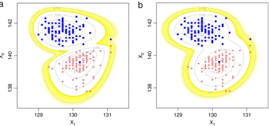
is the maximized log-likelihood,mis the number of parameters andnis the sample size. The comparison results are listed inTable 2. It is readily seen from the table that both AIC and BIC values as well as the LRT statistic consistently favor the SNMIX model.

The contours of the ML-fitted SNMIX and NORMIX densities are depicted inFig. 1. As anticipated, the fitted SNMIX density has better ability to capture the asymmetry and tracks the data more closely than does the fitted NORMIX density.

(8)

Fig. 1. Scatter plot of(X₁,X₂), overlaid on the contours of fitted two-component (a) SNMIX (b) NORMIX models. The genuine old Swiss 1000 franc bills are indicated by the solid circles (•) and the pluses (+) denote the counterfeit ones.

6. Concluding remarks

In this paper I have presented an ML approach to estimating the parameters as well as their information-based standard errors for a multivariate setting of SNMIX models. I have described a stochastic normal-truncated normal-multinomial hierarchical representation of SNMIX and presented an effective EM algorithm for dealing with ML estimation in a flexible complete data framework. The formulae for computing the first two moments of the multivariate truncated normal distribution and their usefulness in computing conditional expectations are also shown. The proposed EM algorithm appears to be easily implemented and coded with existing statistical software such as R package. Numerical results illustrated in Section5indicate that the SNMIX model for the bank data is evidently more adequate than the conventional NORMIX model.

While the SNMIX model considered in this paper has proved its great flexibility in regulating skewness among components, its robustness against outliers could be seriously affected by thick tailed observations. Lin et al. [16] have recently proposed a remedy to accommodate skewness and heavy-tailedness simultaneously using the mixture of skew

t distributions (Azzalini and Capitaino [4]). However, their approach is restricted to data with univariate outcomes. I conjecture that the methodology presented in this paper can be undertaken under a multivariate setting of skewtmixtures and should yield satisfactory results in certain situations, at the expense of additional complexity of implementation. Nevertheless, a deeper investigation of those modifications is beyond the scope of the present paper, but provides interesting topics for further research.

Acknowledgments

The author would like to express his deepest thanks to the Chief Editor, the Associate Editor and two anonymous referees for their insightful comments and valuable suggestions, which led to substantial improvements in the presentation of this work. I am also grateful to Ms. Chiang-Ling Chen for her initial simulation study and to Prof. Jack C. Lee for his kindness and patience in proofreading the earlier version of this paper. This research was partly supported by the National Science Council of Taiwan (Grant NO. NSC95-2118-M-005-001-MY2).

Appendix. Proofs of Eqs.(20)–(22)

Let

`

cj=

`

cj

(

Θ|yj

,

Zj

,

τj

)

denote the complete-data log-likelihood formed from the single observationyj. Thus,

`

cj= g X i=1 Zij logwi− 1 2log|Σi| − 1 2

(

yj−ξi−Λiτj

)

T_Σ−1 i

(

yj−ξi−Λiτj

)

− 1 2τ T jτj

.

Now, recall the formulae for matrix derivatives

∂

log|Σ|

∂

Σ =2Σ

−1₋_Diag

₍

_Σ−1

₎

∂

tr

(

Σ−1A

)

∂

Σ = −2Σ

−1_AΣ−1₊_Diag

₍

_Σ−1_AΣ−1

_),

_(A.1)

(9)

By applying(A.1), the first derivatives of

`

cjwith respect towi,ξi,ΛiandΣiare

∂`

cj

∂

wi = Zij wi −Zgj wg

,

∂`

cj

∂

ξi =ZijΣ −1 i

(

yj−ξi−Λiτj

),

∂`

cj

∂

Λi =ZijΣ−i 1

(

yj−ξi

)

τjT−ΛiτjτTj

,

∂`

cj

∂

Σi = −1 2Zij n 2Σ−i1−Diag

(

Σ −1 i

)

−2Σ −1 i

(

yj−ξi−Λiτj

)(

yj−ξi−Λiτj

)

TΣ −1 i +DiagΣ−_i1

(

y_j−ξ_i−Λiτj

)(

yj−ξi−Λiτj

)

TΣ −1 i o = 1 2Zij 2Aij−Diag

(

Aij

)

,

(A.2) whereAij=Σ −1 i

(

yj−ξi−Λiτj

)(

yj−ξi−Λiτj

)

TΣ −1 i −Σ −1 i .

Now, ifΛiis a diagonal matrix, i.e.,λi=diag

(

Λi

)

, then

∂`

cj

∂

λi = −1 2Zij n −2diagΣ−_i1

(

y_j−ξ_i

)

τT j +2diagΣ−_i1ΛiτjτTj o = Zij n Σ−_i1τ_j

(

y_j−ξ_i

)

T1p−

(

Σ −1 i τjτTj

)

λi o

.

(A.3)

In the case ofΣ1= · · · =Σg=Σ, one obtains

∂`

cj

∂

Σ = − 1 2 g X i=1 Zij n 2Σ−1−Diag

(

Σ−1

)

−2Σ−1

(

y_j−ξ_i−Λiτj

)(

yj−ξi−Λiτj

)

TΣ −1 +DiagΣ−1

(

y_j−ξ_i−Λiτj

)(

yj−ξi−Λiτj

)

TΣ −1o = 1 2Zij 2A∗ ij−Diag

(

A ∗ ij

)

,

(A.4) whereA∗_ij=Σ−1

(

yj−ξi−Λiτj

)(

yj−ξi−Λiτj

)

TΣ−1−Σ−1.

On evaluation atΘ= ˆΘ, taking the conditional expectations of(A.2)–(A.4)yields the score estimates(20)–(22). References

[1] R.B. Arellano-Valle, H. Bolfarine, V.H. Lachos, Bayesian inference for skew-normal linear mixed models, J. Appl. Stat. 34 (2007) 663–682. [2] R.B. Arellano-Valle, M.G. Genton, On fundamental skew distributions, J. Multivariate Anal. 96 (2005) 93–116.

[3] A. Azzalini, A class of distributions which includes the normal ones, Scand. J. Statist. 12 (1985) 171–178.

[4] A. Azzalini, A. Capitaino, Distributions generated by perturbation of symmetry with emphasis on a multivariate skewt-distribution, Roy. Statist. Soc. Ser. B 65 (2003) 367–389.

[5] A. Azzalini, A. Dalla Valle, The multivariate skew-normal distribution, Biometrika 83 (1996) 715–726.

[6] K.E. Basford, D.R. Greenway, G.J. McLachlan, D. Peel, Standard errors of fitted means under normal mixture, Comp. Statist. 12 (1997) 1–17. [7] A.P. Dempster, N.M. Laird, D.B. Rubin, Maximum likelihood from incomplete data via the EM algorithm (with discussion), J. Roy. Statist. Soc. Ser. B 39

(1977) 1–38.

[8] B. Efron, R. Tibshirani, Bootstrap method for standard errors, confidence intervals, and other measures of statistical accuracy, Statist. Sci. 1 (1986) 54–77.

[9] B. Flury, H. Riedwyl, Multivariate Statistics, a Practical Approach, Cambridge University Press, Cambridge, 1988. [10] S. Frühwirth-Schnatter, Finite Mixture and Markov Switching Models, Springer, New York, 2006.

[11] J.A. Hartigan, M.A. Wong, Algorithm AS 136: AK-means clustering algorithm, Appl. Stat. 28 (1979) 100–108. [12] A. Genz, Numerical computation of multivariate normal probabilities, J. Comput. Graph. Statist. 1 (1992) 141–150.

[13] A. Genz, Comparison of methods for the computation of multivariate normal probabilities, Comp. Sci. Statist. 25 (1993) 400–405. [14] A.F. Gupta, G. González-Farías, J.A. Domínguez-Monila, A multivariate skew normal distribution, J. Multivariate Anal. 89 (2004) 181–190. [15] G.P.H. Styan, Hadamard products and multivariate statistical analysis, Linear Algebra Appl. 6 (1973) 217–240.

[16] T.I. Lin, J.C. Lee, W.J. Hsieh, Robust mixture modeling using the skewtdistribution, Statist. Comp. 17 (2007) 81–92. [17] T.I. Lin, J.C. Lee, S.Y. Yen, Finite mixture modelling using the skew normal distribution, Statist. Sinica 17 (2007) 909–927. [18] Y. Ma, M.G. Genton, Flexible class of skew-symmetric distribtions, Scand. J. Statist. 31 (2004) 459–468.

[19] G.J. McLachlan, K.E. Basord, Mixture Models: Inference and Application to Clustering, Marcel Dekker, New York, 1988. [20] G.J. McLachlan, D. Peel, Finite Mixture Models, Wiely, New York, 2000.

[21] R.A. Redner, H.F. Walker, Mixture densities, maximum likelihood and the EM algorithm, SIAM Rev. 26 (1984) 195–239.

[22] S.K. Sahu, D.K. Dey, M.D. Branco, A new class of multivariate skew distributions with application to Bayesian regression models, Canad. J. Statist. 31 (2003) 129–150.

[23] G.M. Tallis, The moment generating function of the truncated multi-normal distribution, J. Roy. Statist. Soc. Ser. B 23 (1961) 223–229. [24] D.M. Titterington, A.F.M. Smith, U.E. Markov, Statistical Analysis of Finite Mixture Distributions, Wiely, New York, 1985.