Image Classification in Content-Based Image Retrieval Systems Based on First Order Color Histogram Features

(1)

International Journal of Emerging Technology and Advanced Engineering

Website: www.ijetae.com (ISSN 2250-2459,ISO 9001:2008 Certified Journal, Volume 4, Issue 11, November 2014)

350

Image Classification in Content-Based Image Retrieval Systems

Based on First Order Color Histogram Features

Abdur Rahman Anas

1

, T. Sravanthi

2

1

M.Tech Communication Systems, Vignana Bharathi Institute of Technology, India

2_{Assistant Professor, Vignana Bharathi institute of Technology, India.}

Abstract— Image Classification in Content-Based Image Retrieval Systems has to be fast and simple in order to provide most efficient color based searches. In order to obtain this in this paper a new approach is introduced based on first order Color histogram features. The main advantage of this method is the very quick generation and comparison of the applied feature vectors. In CBIR systems computation has to be fast and efficient hence primitive features are selected as they can easily generate and compute the applied feature vectors and feature spaces. Our results illustrate the efficacy of loop approach to image characterization and the ability of our approach to adapt the retrieval process image domain through the application of machine learning algorithms.

Keywords— Color Histogram Features, Distance and Similarity measures, Feature vectors, Image Classification.

I. INTRODUCTION

If the images are classified within the database on the basis of particular aspects like color, texture, shape, etc. then it would be very useful and efficient if the images are retrieved using content based image retrieval (CBIR) systems. For example in a large input database the images can be divided into such classes as follows: landscapes, buildings, indoor images, faces, artificial images, etc.

In this paper we have used feature vectors in order to reduce the computation time and decrease the bulk processing required. As we know that computing each and every image bit by bit is more computational hence we have used first order color histogram features like mean, standard deviation, skewness, energy, entropy, kurtosis as feature vectors in generating the feature values of the images. The advantage of this approach is the comparison of histogram features is much faster and more efficient than other commonly used methods. Histogram search characterizes an image by its color distribution, or histogram. Many histogram distances have been used to define the similarity of two color histogram representations. Euclidean distance and its variations are the most commonly used. we have used two more methods other than Euclidean distance, based on distance and similarity measures they are city block distance and tanimoto metric respectively.

In Section 2 the theoretical concepts of our approach are introduced. In Section 3 the experimental analysis has been discussed, and in Section 4 we wrote the conclusions and possible future works.

II. THEORETICAL CONCEPTS

The general concept of our project along with relevant details will be discussed in the following sections.

How the images are classified? What is the concept behind feature extraction and how the images are retrieved?

A. First order Color histogram features

An "image histogram" is a type of histogram that acts as a graphical representation of the tonal distribution in a digital image. It plots the number of pixels for each tonal value. By looking at the histogram for a specific image a viewer will be able to judge the entire tonal distribution at a glance. In image processing and photography, a color histogram is a representation of the distribution of colors in an image. For digital images, a color histogram represents the number of pixels that have colors in each of a fixed list of color ranges that span the image color space, the set of all possible colors.

The shape of the histogram provides us with information about the nature of the image, or sub image if we are considering an object within the image. For example, a very narrow histogram implies a low contrast image, a histogram skewed toward the high end implies a bright image, and a histogram with two major peaks, called bimodal, implies an object that is in contrast with the background. If the set of possible color values is sufficiently small, each of those colors may be placed on a range by itself; then the histogram is merely the count of pixels that have each possible color. Most often, the space is divided into an appropriate number of ranges, often arranged as a regular grid, each containing many similar color values. The color histogram may also be represented and displayed as a smooth function defined over the color space that approximates the pixel counts.

(2)

International Journal of Emerging Technology and Advanced Engineering

351

These statistical features provide us with information about the characteristics of the intensity level distribution for the image. We define the first-order histogram probability, P(g), as:

P(g) = N(g)/M……….(1)

M is the number of pixels in the image (if the entire image is under consideration then M = N2 for an N × N image), and N(g) is the number of pixels at gray level g. As with any probability distribution all the values for P(g) are less than or equal to 1, and the sum of all the P(g) values is equal to1.

The features based on first order color histogram are mean, standard deviation, skewness, energy, entropy, kurtosis which are illustrated below.

The mean is the average value, so it tells us something about the general brightness of the image. A bright image will have a high mean, and a dark image will have a low mean.

Mean GL = sum(GLs .* pixel Counts) /number of Pixels;………..(2)

The standard deviation, which is also known as the square root of the variance, tells us something about the contrast. It describes the spread in the data, so a high contrast image will have a high variance, and a low contrast image will have a low variance.

sd = sqrt(variance GL);………..(3)

Skewness is a measure of symmetry, or more precisely, the lack of symmetry. A distribution, or data set, is symmetric if it looks the same to the left and right of the center point. The skewness for a normal distribution is zero, and any symmetric data should have a skewness near zero. Negative values for the skewness indicate data that are skewed left and positive values for the skewness indicate data that are skewed right. By skewed left, we mean that the left tail is long relative to the right tail.

Skewness= sum((GLs – mean GL) .^ 3 .* pixel Counts) / ((number Of Pixels - 1) * sd^3);…(4)

Energy is defined based on a normalized histogram of the image. Energy shows how the gray levels are distributed. When the number of gray levels is low then energy is high.





 L-1 0 g

[P(g)] ENERGY

………(5)

The entropyis a measure that tells us how many bits we need to code the image data. An image that is perfectly flat will have an entropy of zero. Consequently, they can be compressed to a relatively small size. On the other hand, high entropy images such as an image of heavily cratered areas on the moon have a great deal of contrast from one pixel to the next and consequently cannot be compressed as much as low entropy images.





L-1

0 g

2

[

(

)]

P(g)log

ENTROPY

P

g

…..(6)

Kurtosis is a measure of whether the data are peaked or flat relative to a normal distribution. That is, data sets with high kurtosis tend to have a distinct peak near the mean, decline rather rapidly, and have heavy tails. Data sets with low kurtosis tend to have a flat top near the mean rather than a sharp peak. A uniform distribution would be the extreme case

Kurtosis = sum((GLs – mean GL) .^ 4 .* pixel Counts) / ((number Of Pixels - 1) * sd^4); …….(7)

B. Feature Extraction

In image processing, feature extraction is a special form of dimensionality reduction. When the input data to an algorithm is too large to be processed and it is suspected to be very redundant (e.g. the same measurement in both feet and meters, or the repetitiveness of images presented as pixels), then the input data will be transformed into a reduced representation set of features (also named features vector). Transforming the input data into the set of features is called feature extraction. If the features extracted are carefully chosen it is expected that the features set will extract the relevant information from the input data in order to perform the desired task using this reduced representation instead of the full size input. If the template image has strong features, a feature-based approach may be considered; the approach may prove further useful if the match in the search image might be transformed in some fashion. Since this approach does not consider the entirety of the template image, it can be more computationally efficient when working with source images of larger resolution, as the alternative approach.

(3)

International Journal of Emerging Technology and Advanced Engineering

352

The measurements may be symbolic, numerical, of both. An example of a symbolic feature is color such a ‖blue‖ or ‖red‖; an example of a numerical feature is the area of an object.

The vector space associated with these vectors is often called the feature space. In order to reduce the dimensionality of the feature space, a number of dimensionality reduction techniques can be employed.

For n-dimensional feature vectors it is an abstract mathematical construction called a hyperspace. As we shall see the creation of the feature space allows us to define distance and similarity measures which are used to compare feature vectors and aid in the classification of unknown samples.

C. Classification Mechanism

As we need to classify the objects we are using feature vectors, but we need some other method in order to classify. These methods are mainly introduced in order two compare the two feature vectors. The primary methods are to either measure the difference between the two, or to measure the similarity. The two vectors that are closely related will have more similarity and less difference.

The difference can be measured by a distance measure in the n-dimensional feature space; the bigger the distance between two vectors, the greater the difference. This is the distance between each and every pixel in the image, here in my project the distance is measured between each and every feature vector. Then this distance values are compared with all other values. This values gives amount of distance they are apart, more the value is then accordingly most similar they are hence more magnitude values are set apart and the relevant images are shown as retrieved images. Based on the different calculation phenomena there are few methods in distance measure as followed?

Euclidean distance (most common metric), The Euclidean distance is the straight-line distance between two pixels. Given A and B are two vectors where

A=                    

a

n . . . 2 1 and B=                    

b

n . . . 2 1

Then the Euclidean distance is given by:



  n i i i b a 1 2 ) ( ………….(8)

City block of absolute value metric, The city block distance metric measures the path between the pixels based on a 4-connected neighborhood. Pixels whose edges touch are 1 unit apart; pixels diagonally touching are 2 units apart.

Using A and B as above the city block distance is given as







n i i i

b

a

1 ……….(9)

This metric is computationally faster than the Euclidean distance, but gives similar results. A distance metric that considers only largest difference is the maximum value

metric defined by:







a



b

,

a



b

,....,

a

n



b

n



max

1 1 2 2

..(10)

Generalized distance metric is the Minkowski distance, it is a metric of Euclidean space which can be considered as a generalization of both the Euclidean distance and the Manhattan distance Minkowski distance is typically used with r being 1 or 2. The latter is the Euclidean distance, while the former is sometimes known as the Manhattan distance. In the limiting case of r reaching infinity, we obtain the Chebyshev distance given as

r n i r i i

b

a

/ 1

1

















 ₍₁₁₎

Where r is a positive integer

Chebyshev distance (or Tchebychev distance), maximum metric, or L∞ metric[1] is a metric defined on a vector space where the distance between two vectors is the greatest of their differences along any coordinate dimension, this metric is given as:







n i i i

b

a

1

)

max(

……….(12)

(4)

International Journal of Emerging Technology and Advanced Engineering

353

Usually similarity measures are in some sense the inverse of distance metrics: they take on large values for similar objects and either zero or a negative value for very dissimilar objects.

The most common form of the similarity measure is the

vector inner product. It is an algebraic operation that takes two equal-length sequences of numbers (usually coordinate vectors) and returns a single number. This operation can be defined either algebraically or geometrically. Algebraically, it is the sum of the products of the corresponding entries of the two sequences of numbers. Using our definitions for the two vectors A and B, we can define the vector inner product by the following equation:





n

i

i i

b

a

1 _{………..(13)}

Another commonly used similarity measure is the

Tanimoto metric, defined as:



 







n

i i i n

i i n

i i

n

i i i

b

a

b

a

b

a

1 1

2

1 2

1

…….(14)

This metric takes on values between 0 and 1, which can be thought of as a ‖percent of similarity‖ since the value is 1 (100%) for identical vectors and gets smaller as the vectors get farther apart. The Tanimoto Coefficient uses the ratio of the intersecting set to the union set as the measure of similarity.

D. Algorithms and methods for feature vector comparison

The simplest comparing algorithm is nearest neighbor method. This method compares each and every template present in the vector and gives results based on the distance measure or similarity measure. This method gives small number which will be less if it is distance method and more for similarity measure for closely related vectors. The nearest neighbor algorithm is easy to implement and executes quickly, but it can sometimes miss shorter routes which are easily noticed with human insight, due to its "greedy" nature. In the worst case, the algorithm results in a tour that is much longer than the optimal tour.

We can make nearest neighbor method more complicated by selecting group of bits and comparing with every other group.

This method is called K-nearest neighbor method in this method group of close feature vectors are considered from the image and are compared with other images for distance and similarity measure.

We can reduce the complexity even further by considering nearest centroid method. In this method a nearest centroid is calculated for every class of images and compares them with representative centroids of other images. The nearest centroid is calculating the average of all the values present in the feature space or feature vector.

III. PERFORMANCE ANALYSIS OF IMAGE CLASSIFICATION

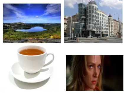
In this project we have considered 50 images of four different classes. In this project for experimental analysis we have considered classes like landscapes, buildings, face and coffee cups. For each query image we have selected 10 images of same image class for experimental output to be clear. In this project as we are YCC model for signal efficiency we get three different color characteristics depending on that different feature vectors are obtained for each image. From the experiment we have obtained 15 feature vectors for a single image.

The query images considered in my project are designated with the class test template itself. The four image classes used in my project are as shown:

[image:4.612.343.553.432.590.2]

Fig 1: query image of each class namely landscape, building, coffee cup, face.

(5)

International Journal of Emerging Technology and Advanced Engineering

354

The algorithms were coded in MATLAB, because this system is rather computationally fast and efficient the code generation is very simple and also we easier access to the storage files easily.

The matlab code for first order color histogram feature calculation is as shown below:

function t=histprp(hst,N);

t.m=sum([1:N]'.*hst);

t.s=sqrt(sum(([1:N]'-t.m).^2.*hst)); t.sk1=sum(([1:N]'-t.m).^3.*hst)/t.s.^3; mode=find(hst==max(hst));

sk2=(t.m-mode(cell(length(mode)/2)))/t.s; t.er=sum(hst.^2);

t.ep=-sum(hst.*log2(hst+eps)); t.k=kurtosis(hst);

Fig 2: Matlab code first order color histogram feature generation. IV. CONCLUSION

In this project a new approach of color image classification was introduced, where different color signal of YCBCR is used. By doing this, subsequent image/video processing, transmission and storage can do operations and introduce errors in perceptually meaningful ways. The main advantage of this method is the usage of simple first order image features, as histogram features. Histogram features can be generated from the image histogram very quickly and the comparison of these features is computationally fast and efficient.The features used in this project are first order color histogram features like mean, standard deviation, skewness, kurtosis, energy, entropy. These features are considered as feature vectors in order to compare the images. The primary methods are to either measure the differencebetween the two, or to measure the similarity. Two vectors that are closely related will have a small difference and a large similarity.

This project can also implemented by using different semantic features but efficiency is important hence we need to consider more than two different semantic features like space or region along with the histogram features.

We can also implement the project using higher order histogram features where computation will be high hence time and efficiency may vary. This project can also be implemented using domain specific features like face recognition, finger print matching etc. as feature vectors for classifying the images.

REFERENCES

[1] Esmat Rashedi, Hossein Nezamabadi-pour, Saeid Saryazdi, ―A simultaneous feature adaptation and feature selection method for content-based image retrieval systems‖, Knowledge-Based Systems 39, 2013.

[2] Fazal-E-Malik and Baharum Bin Baharudin, ―Mean And Standard Deviation Features Of Color Histogram using Laplacian Filter For Content-Based Image Retrieval‖,Journal of Theoretical and Applied Information Technology, Vol. 34 No.1.15th December 2011. [3] Sz. Sergy´an, ―Color Content-based Image Classification,‖ 5th

Slovakian-Hungarian Joint Symposium on Applied Machine Intelligence and Informatics, Poprad, Slovakia, pp. 427–434, 2007. [4] SHI Dongcheng, XU Lan, HAN Ungyan, ―Image retrieval using

both color and texture features‖, The Journal Of China Universities Of Posts and Telecommunications, October 2007.

[5] Prof. Dr.-Ing. H. Ney and Thomas Deselaers Matrikel nummer, ―Features for Image Retrieval‖, 2003.

[6] A.W.M. Smeulders, M. Worring, S. Santini, A. Gupta, R. Jain, ―Content-Based Image Retrieval at the End of the Early Years,‖ IEEE Transactions on Pattern Analysis and Machine Intelligence, vol. 22, no. 12, pp. 1349–1380, 2000.

[7] C. Carson, M. Thomas, S. Belongie, J.M. Hellerstein, J. Malik, ―Blobworld: A System for Region-Based Image Indexing and Retrieval,‖ Third International Conference on Visual Information Systems, Springer, 1999.

[8] SAMI 2008 • 6th International Symposium on Applied Machine Intelligence and Informatics

[9] S. Aksoy. A Probabilistic Similarity Framework for Content-Based Image Retrieval. PhD thesis, University of Washington, Seattle, WA, June 2001.

[10] A. P. Berman and L. G. Shapiro. A flexible image database system for content-based retrieval. Computer Vision and ImageUnderstanding, 75(1/2):175–195, 1999.