Exploiting structure of maximum likelihood estimators for extreme
value threshold selection
J. L. Wadsworth
Statistical Laboratory, University of Cambridge, U.K.
December 1, 2014
Abstract
In order to model the tail of a distribution, one has to define the threshold above or below which an extreme value model produces a suitable fit. Parameter stability plots, whereby one plots maximum likelihood estimates of supposedly threshold-independent parameters against threshold, form one of the main tools for threshold selection by practitioners, principally due to their simplicity. However, one repeated criticism of these plots is their lack of interpretability, with pointwise confidence intervals being strongly dependent across the range of thresholds. In this article, we exploit the independent-increments structure of maximum likelihood estimators in order to produce complementary plots with greater interpretability, and a suggest simple likelihood-based procedure which allows for automated threshold selection.
Keywords: diagnostic plots; extreme value modelling; maximum likelihood; threshold selection.
1
Introduction
When faced with the problem of making inferences on the tail of a distribution, one usually invokes the extreme value modelling paradigm. In this article we will focus on upper tails; theory for lower tails is symmetric in generality. Suppose that we are able to assume a sequence of identically distributed random
variables,{Xi∼F}ni=1, satisfying a long-range weak dependence condition (Leadbetter et al., 1983, Ch. 3),
and let xF := inf{x : F(x) >0} and xF := sup{x : F(x)< 1} be the lower and upper endpoints of the
support. For a wide variety ofF, the distribution of appropriately scaled excesses,Xi−u, over the threshold
u, converges to the generalized Pareto (GP) distribution, with distribution function (d.f.)
asu→xF (Pickands, 1975; Davison and Smith, 1990). At a practical level this leads to the approximation
P(Xi> x|Xi> u)≈[1 +ξ(x−u)/σu] −1/ξ
+ for a high thresholdu, withξ∈Ra shape parameter andσu>0
a threshold-dependent scale parameter to be estimated; the case ξ= 0 is to be interpreted in the limiting
sense.
For a givenF, if scaled threshold excesses follow a limiting GP distribution, then appropriately normalized
maxima Mn := max{X1, . . . , Xn} converge to following the generalized extreme value (GEV) distribution
asn→ ∞, with d.f.
G(x) = expn−[1 +ξ(x−µ)/σ]−1/ξ+ o, µ∈R, σ >0, ξ∈R,
with the shape parameterξbeing the same in bothGandH. Again the GEV is treated as the approximate
distribution ofMnfor a large but finite sequence lengthn. However, if all data are available then a
threshold-based modelling approach is usually preferred due to efficiency gains from an increased sample size. These two results can be derived from a unifying point process representation due to Pickands (1971). If
there exist normalization sequences{an >0},{bn∈R} such that the sequence of point processes,
Pn= i n+ 1, Xi−bn an :i= 1, . . . , n d → P, n→ ∞, (1)
withP a non-trivial limit on (0,1)×(bl= limn→∞(xF−bn)/an,∞), thenP is a non-homogeneous Poisson
process (NHPP) with integrated intensity measure
Λ{(a, b)×(x,∞)}= (b−a) [1 +ξ(x−µ)/σ]−1/ξ+ , µ∈R, σ >0, ξ∈R, 0≤a < b≤1.
The link between the point process result and the GP and GEV distributions is explained in Coles (2001,
Sect. 7.4), for example. In the convergence (1), only points for whichXiis extreme are retained in the limit,
and at a statistical level this motivates the use of the NHPP model for data exceeding a high threshold. The
parameters (µ, σ, ξ) are respectively location, scale and shape parameters to be estimated, with ξ as inG
andH. The NHPP model has the advantage over the GP model of accounting for the rate of exceedances
over the threshold, and having a threshold-independent parameterization; we thus focus on this modelling strategy.
The first task in inference is to decide upon a threshold for which the approximation is adequate, taking into account the familiar bias-variance trade-off: lower thresholds induce higher bias but lower estimation variance, and vice versa. There is a growing wealth of literature devoted both to the problem of fixed threshold selection, and incorporating uncertainty in threshold selection into the inference; a recent review
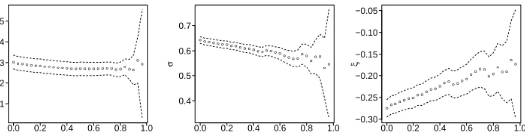
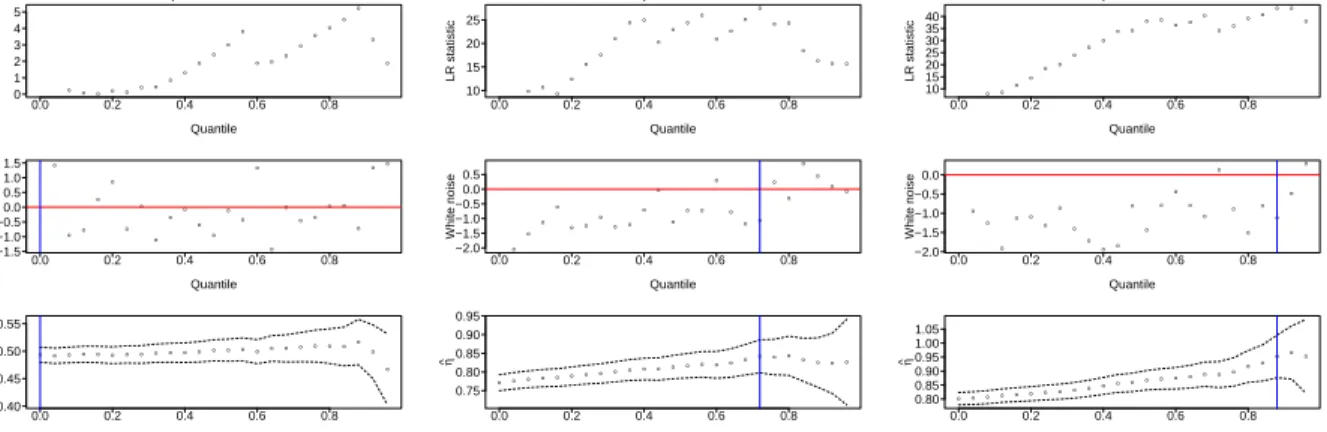
●● ● ● ●● ● ● ● ● ● ● ● ● ● ● ● ● ● ● ● ● ●● ●●● ● ● ● 0.0 0.2 0.4 0.6 0.8 1.0 1.1 1.2 1.3 1.4 1.5 Quantile µ ●● ● ●● ● ●● ● ● ● ●● ● ● ● ● ●●●●● ● ●● ● ● ● ● ● 0.0 0.2 0.4 0.6 0.8 1.0 0.4 0.5 0.6 0.7 Quantile σ ●● ● ●●● ● ● ●● ● ●● ●● ● ● ●● ●● ● ● ●● ● ● ● ● ● 0.0 0.2 0.4 0.6 0.8 1.0 −0.30 −0.25 −0.20 −0.15 −0.10 −0.05 Quantile ξ
Figure 1: Traditional parameter stability plots for (µ, σ, ξ) in the NHPP model.
is provided by Scarrott and MacDonald (2012). In this article, we treat only the first of these issues, whilst acknowledging the importance of the latter. One of the main tools used in fixed threshold selection is the parameter stability plot: if suitable convergence has been achieved towards the limit model, then estimates
of parameters (µ, σ, ξ) should be stable across a range of thresholds. The parameter stability plot consists
of parameter estimates plotted against a range of thresholds, with pointwise confidence intervals. One then selects as a threshold the lowest value above which the parameters are deemed to be constant, attempting to take into account the uncertainty in their estimation. An example is presented in Figure 1; the difficulty in
interpretation is evident. Of these three plots, those forσandξtell a similar story, whilst that forµoffers
little information. In the following, we thus focus mainly on plots for ξ; some further comments on this are
given in Section 5.
In spite of the complaint that dependent confidence intervals are difficult to account for (as mentioned for instance by Scarrott and MacDonald (2012), Wadsworth and Tawn (2012) and Northrop and Coleman
(2014)), thesimplicityof parameter stability plots still renders their use commonplace. To produce them, one
simply needs to fit the model above a range of thresholds. By contrast, to use any of the more “sophisticated” methods proposed in the literature (e.g. Beirlant et al., 1999; Ferreira et al., 2003; Wadsworth and Tawn, 2012; Northrop and Coleman, 2014, to list only a few), one needs to study more complicated methodology and / or implement bespoke code. Our aim in this article is to address the interpretability issue of parameter stability plots by exploiting the asymptotic distributional theory of the joint distribution of maximum likelihood estimators (MLEs) from overlapping samples of data, to produce diagnostics which do not require any further modelling assumptions. Furthermore, a simple testing procedure is suggested, to allow automated threshold selection if desired.
The issue of threshold selection is most commonly associated to univariate extreme value theory. However, when one wants to model the extremal dependence between two or more variables, there is typically a choice of dependence threshold as well. In the bivariate setting, an assessment of the level of dependence between two
as follows. Suppose that random variables (XE, YE) have been transformed to have standard exponential
margins. Then a widely-applicable regular variation assumption yields
P{min(XE, YE)> x+t|min(XE, YE)> t}=
L(ex+t)
L(et) exp(−x/η), (2)
with L slowly-varying at infinity, i.e., limt→∞L(tx)/L(t) = 1, for x > 0. Values of η > 1/2, and η <
1/2 indicate positive and negative extremal association respectively, whilst η = 1/2 corresponds to near
independence. The caseη = 1 is of special importance as this is implied by the variables beingasymptotically
dependent, whilstη <1 implies asymptotic independence. Different modelling strategies can be applicable
to these two scenarios; see Coles (2001, Ch. 8), or Beirlant et al. (2004, Ch. 9) for further details. To
estimateη, equation (2) implies an approximate exponential model for large x > u: P{min(XE, YE)> x|
min(XE, YE)> u} ≈exp{−(x−u)/η}. A suitable dependence thresholdumay again be determined through
parameter stability plots for the exponential distribution inverse rate parameterη. We will also consider this
problem in the sequel. Threshold selection for multivariate problems is also considered in Lee et al. (2013), but starting from an assumption of asymptotic dependence.
The remainder of the article is as follows. In Section 2 we give details of the asymptotic joint distribution of the MLEs, and use this to suggest alternative diagnostic plots. In Section 3 we outline a simple testing procedure that would allow for automated threshold selection on multiple datasets; properties and perfor-mance are assessed through simulation. Finally we consider the perforperfor-mance of the methods on a variety of freely-available datasets, so that the reader can compare easily with their own assessment. R code is available as supplementary material.
2
Asymptotic joint distribution of MLEs
2.1
Set-up and notation
Let us denote by θ ∈ Θ ⊆ Rp the parameters of our model, with θ
0 an assumed true value. We wish
to estimateθ0 from data X, which follow a probability model with density fθ0; we assume that sufficient
regularity conditions for asymptotic consistency and normality of the maximum likelihood estimators hold.
Suppose that the observations Xi are mutually independent, and that each Xi ∈ R, for some interval or
regionR. For our purposes,Rcan usually be considered as (u1,∞), though the theory applies more generally.
The joint distribution of score functions from overlapping samples is known and used in the area of sequential analysis (e.g. Siegmund (1985, p.65), or Cook and DeMets (2008, Sect. A.5)), but to our knowledge has not been exploited in this context. Since we have not found a derivation suited to our objectives, and in order
to provide a reference on the topic, the key results will be stated here, whilst simple derivations are given as supplementary material.
If X is of random lengthN and (X, N) represent realizations from a NHPP, with intensityλθ(x) and
integrated intensity Λθ(R) =
R
Rλθ(x)dx, then the likelihood function on the regionRis
LR(θ) :=fθ(x) = (N Y i=1 λθ(xi) ) exp{−Λθ(R)}. (3)
Alternatively, if X is of fixed length n, consisting of independent random variables each with marginal
densityfθ,1, then the likelihood function is simply
LR(θ) = n
Y
i=1
fθ,1(xi). (4)
Now suppose that we partitionRinto R1, . . . , Rk, allowing us to define several nested regions
¯ Ri:= k [ j=i Ri,
so thatR= ¯R1⊃R¯2⊃ · · · ⊃R¯k =Rk. For our purposes, these regions will be (u1,∞), (u2,∞), . . . ,(uk,∞),
withu1< u2 <· · ·< uk. Denote by ˆθi the MLE derived from observations on ¯Ri = (ui,∞), and let Ii be
the Fisher information matrix on ¯Ri, withIi−1 its inverse.
2.2
Joint distribution
For notational convenience, we firstly state the results for a Poisson process, then detail the modifications required for likelihoods of the form (4). Since asymptotic results require that the number of points tends to
infinity, but the parameters remain fixed, consider a superposition ofmPoisson processes. Then, with the
above set-up and notation, asm→ ∞
m1/2( ˆθ 1−θ0) m1/2( ˆθ 2−θ0) .. . m1/2( ˆθ k−θ0) d →Npk(0,Σ), Σ = {I−1}min(i,j) 1≤i≤k,1≤j≤k. (5)
Thepk×pk covariance matrix Σ therefore has a block structure, with the blocks being the inverse Fisher information matrices. Here the Fisher information is
Ii =E{−∇2logLR¯i(θ0)}=−Λθ0( ¯Ri)E{∇
2logλ
θ0(X)}+∇
2Λ θ0( ¯Ri),
the final expectation being with respect to the densityλθ0/Λθ0( ¯Ri).
The result is essentially the same for a likelihood of the form (4), where, given m1 points on ¯R1, the
number of points on ¯Ri isMi∼Binomial(m1,P(X ∈R¯i|X∈R¯1)). In (5) above, replacingmin theith row
byE(Mi) =m1P(X ∈R¯i|X ∈R¯1) yields the same convergence, with
Ii=−E{∇2logfθ0,1(X)},
expectation being with respect to the densityfθ0,1.
2.3
Consequences of the joint distribution
We consider two consequences of the asymptotic distribution (5). The first of these is an independent
increments structure to the MLEs, the second is a sequence of independent estimators, centered aroundθ0.
From this point onwards, distributions are assumed to hold approximately for finite m, mi etc., and these
values appear in the variances.
2.3.1 Independent increments An immediate consequence of (5) is ( ˆθ1−θˆ2) ( ˆθ2−θˆ3) .. . ( ˆθk−1−θˆk) . ∼Np(k−1) 0, 1 mBlockDiag I −1 i+1−I −1 i 1≤i≤k−1 . (6)
It is clear from (6) that, with estimates of the Fisher information matrices, pre-multiplication by the Cholesky factor of the covariance matrix would yield approximately independent normal random variables. In
partic-ular, if we isolate a parameter of interest,ξin our case, and denote bym−1{(I−1
i+1−I −1
variance of ˆξi−ξˆi+1, then the standardized increments ξ1∗ ξ2∗ .. . ξ∗k−1 :=m1/2 ( ˆξ1−ξˆ2) {(I−1 2 −I −1 1 )ξ,ξ}1/2 ( ˆξ2−ξˆ3) {(I−1 3 −I −1 2 )ξ,ξ}1/2 .. . ( ˆξk−1−ξˆk) {(I−1 k −I −1 k−1)ξ,ξ}1/2 . ∼Nk−1(0,1k−1),
with 1n denoting the n-dimensional identity matrix. That is, asymptotically, ξ∗ = (ξ1∗, . . . , ξ∗k−1)T is a
sequence of independent standard normal random variables, hence we shall refer to ξ∗ as the white noise
process. This distribution is valid on an assumption that ξ >−1/2, since Smith (1985) showed that this is
necessary for maximum likelihood estimators from extreme value models to behave regularly.
One often expects that MLEs from furthest into the data, ˆξ1,ξˆ2, . . ., are larger or smaller than those
estimated using the most extreme data, with a gradual move towards stability around a constant value from
estimates derived from further into the tail. This is explained by the so-calledpenultimate theoryof extremes,
described by Gomes (1994) or Smith (1987); a brief summary of the latter is also given in Wadsworth and Tawn (2012). As a consequence, one might anticipate that departures from the null assumption of the white
noise process forξ∗ are manifested as too many large or small values from estimates furthest into the body
of the data. This is indeed often the case, and is the motivation for the likelihood-based automated selection procedure introduced in Section 3.
2.3.2 Independent estimators of θ0
A second use of (5) is to create a sequence of independent estimators that are still centered around θ0.
Let i : j denote the sequence of indices {i, i+ 1, . . . , j}; ˆθi:j denote the p(j−i+ 1)-vector of estimators
( ˆθi, . . . ,θˆj)T;Jk−j,pbe thep(k−j)×pmatrix composed ofk−jvertically stacked copies of 1p, and let Σs,t
denote the submatrix of Σ with rows and columns indexed by sequencessand t, respectively. Then, using
well-known properties of the multivariate normal, one has
ˆ θj−Σj,j+1:kΣ−1j+1:k,j+1:kθˆj+1:k . ∼Np θ0−Σj,j+1:kΣ−1j+1:k,j+1:kJk−j,pθ0, 1 m(Σj,j−Σj,j+1:kΣ −1 j+1:k,j+1:kΣj+1:k,j) ,
and this variable is independent of ˆθj+1:k. Therefore, defining
˜
θj:= (1p−Σj,j+1:kΣ−1j+1:k,j+1:kJk−j,p)
−1( ˆθ
and ˜θk = ˆθk, the sequence of estimators ( ˜θ1, . . . ,θ˜k) is asymptotically normal, centered around θ0, with Var( ˜θj) equal to (1p−Σj,j+1:kΣ−1j+1:k,j+1:kJk−j,p) −11 m(Σj,j−Σj,j+1:kΣ −1 j+1:k,j+1:kΣj+1:k,j)(1p−Σj,j+1:kΣ−1j+1:k,j+1:kJk−j,p) −T,
andCov( ˜θi,θ˜j) = 0, j6=i. This suggests a plot of the adjusted estimates of our parameter of interest, ˜ξ,
or ˜η, against threshold. We include an example of such a plot in Section 3.2.3, but we have found the use of
the null white noise processξ∗ more useful in practice, and thus we focus mainly on that.
3
Likelihood ratio test and simulation results
3.1
Likelihood ratio testing for white noise
As detailed in Section 2.3.1, the null (i.e., when the data arise from the assumed extreme value model)
asymptotic distribution of the increment processξ∗ is a sequence of independent standard normal random
variables, and due to the structure of extreme value theory problems, we expect departures from this null distribution to be more frequent from estimates derived further into the body of the distribution. That is,
we expect thatξ∗1:j is less likely to be white noise thanξj+1:k−1∗ . With this in mind, consider the following
simple changepoint model forξ∗:
ξ∗i ∼N(β, γ) iid, i= 1, . . . , j,
ξ∗i ∼N(0,1) iid, i=j+ 1, . . . , k−1,
(7)
based on a simplistic assumption that below an appropriate threshold, ξ1:j∗ might be better approximated
by aN(β, γ) distribution than aN(0,1) distribution. Some motivation for this is provided by the fact that
under model misspecification, estimators are often still asymptotically normal, but with adjusted means and covariances (White, 1982). The likelihood function associated to (7) is:
L(β, γ, j) = k−1 Y i=1 φ(ξ∗i;β, γ)1(i≤j)φ(ξ∗i; 0,1)1 (i>j) , β ∈R, γ >0, j∈ {2, . . . , k−1}, (8)
with φ(·;β, γ) theN(β, γ) probability density function. To identify a threshold that provides the best fit
to the likelihood (8), we maximize the profile likelihoodLp(j) =L( ˆβj,γˆj, j), with ( ˆβj,ˆγj) the MLEs for a
fixedj. Letj∗ = arg maxjLp(j). The question of interest is then: “doesL( ˆβj∗,γˆj∗, j∗) give a significantly
better fit toξ∗ than L(0,1,0)?”, whereL(0,1,0) =Qk−1
i=1 φ(ξ ∗
likelihood ratio test, with test statistic
T =L( ˆβj∗,ˆγj∗, j
∗)
L(0,1,0) . (9)
The null distribution of T is calculated easily by simulation. If the value of T is significant at some
user-defined level α, then there is evidence against a hypothesis of white noise, and we select as a threshold
that which provides the best fit to (8), u∗ = uj∗+1. (The indexing means that we associate ξj∗ = ( ˆξj−
ˆ
ξj+1)/{(Ij+1−1 −I −1
j )ξ,ξ}1/2 with the higher of the two thresholds involved.) Otherwise there is no evidence
that the sequence ξ∗ is different from white noise, and we take the lowest threshold in contention. This
procedure echoes maximum likelihood changepoint estimation (Eckley et al., 2011, Section 10.2.1).
One possible criticism of this approach is that we approximate what we suppose may often be smooth change towards white noise with a simpler changepoint model. However, since the departures from white noise are generally unknown, this approach at least provides a parsimonious approximation to reality. The
lowest threshold that one entertains, u1, may also have an impact upon the selected threshold, and might
thus be regarded as a tuning parameter. To counteract any effect of this, the testing procedure could be
iterated if desired by re-definingj∗+ 1 = 1, but we do not consider this further here.
A natural question that arises is how many thresholdskone should choose. There should be some link to
the sample size of the data: ifkis too large compared to the sample sizen, then the asymptotic theory will
not provide a good approximation to the distribution. One way to test this is to examine the distribution
of p-values associated to T under the null hypothesis for a variety ofn and k; the distribution should be
uniform when the approximation is adequate.
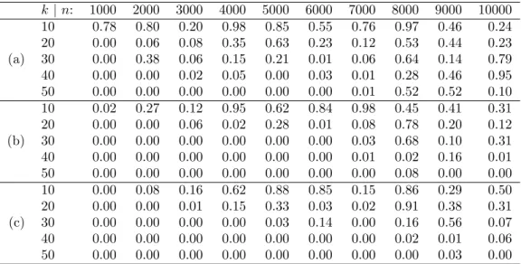
Table 1 offers some insight into reasonable ranges of k and n, displaying approximate p-values from
Kolmogorov–Smirnov tests of uniformity of the p-value distribution, when the LR test was applied under the null hypothesis. The three different sections of the table correspond to two different parameterizations of the exponential model, and the NHPP model. Interestingly, the picture is slightly different between the two
exponential cases: for the inverse rate (η) parameterization, ngenerally needs to be larger for a givenkfor
the distributional results to be accurate. The table is intended as a guide only, as the Kolmogorov–Smirnov test produces only approximate p-values in the presence of ties, which occur here due to p-values being
derived from simulated distributions. Furthermore, the algorithm used is such that k may be reduced in
case of numerical failure as described in Section 3.2.1. In Section 3.2 we take k= 25 for n = 5000, which
appears adequate. In the case of measured data, which are inherently less smooth than simulated data, the
choice ofk may give more variable results; some further comments on this are made in Section 5.
k |n: 1000 2000 3000 4000 5000 6000 7000 8000 9000 10000 10 0.78 0.80 0.20 0.98 0.85 0.55 0.76 0.97 0.46 0.24 20 0.00 0.06 0.08 0.35 0.63 0.23 0.12 0.53 0.44 0.23 (a) 30 0.00 0.38 0.06 0.15 0.21 0.01 0.06 0.64 0.14 0.79 40 0.00 0.00 0.02 0.05 0.00 0.03 0.01 0.28 0.46 0.95 50 0.00 0.00 0.00 0.00 0.00 0.00 0.01 0.52 0.52 0.10 10 0.02 0.27 0.12 0.95 0.62 0.84 0.98 0.45 0.41 0.31 20 0.00 0.00 0.06 0.02 0.28 0.01 0.08 0.78 0.20 0.12 (b) 30 0.00 0.00 0.00 0.00 0.00 0.00 0.03 0.68 0.10 0.31 40 0.00 0.00 0.00 0.00 0.00 0.00 0.01 0.02 0.16 0.01 50 0.00 0.00 0.00 0.00 0.00 0.00 0.00 0.08 0.00 0.00 10 0.00 0.08 0.16 0.62 0.88 0.85 0.15 0.86 0.29 0.50 20 0.00 0.00 0.01 0.15 0.33 0.03 0.02 0.91 0.38 0.31 (c) 30 0.00 0.00 0.00 0.00 0.03 0.14 0.00 0.16 0.56 0.07 40 0.00 0.00 0.00 0.00 0.00 0.00 0.00 0.02 0.01 0.06 50 0.00 0.00 0.00 0.00 0.00 0.00 0.00 0.00 0.03 0.00
Table 1: Approximate p-values from Kolmogorov–Smirnov tests for uniformity of the p-value distribution of the LR test, under the null hypothesis, using (a) the exponential distribution with rate parameterization;
(b) the exponential distribution with inverse rate parameterization (η); (c) the NHPP model.
have detailed here is motivated by the structure of an extreme value problem, and the kind of departures we expect to see from the null distribution, but we make no claim of optimality. Nonetheless, performance in simulation studies appears adequate, and broadly in agreement with values suggested by reasonable inter-pretation of traditional parameter stability plots. Thus the testing procedure could be used for automated threshold selection on multiple datasets if desired.
3.1.1 Contrast with other approaches
Two recent approaches to improving threshold diagnostic plots and / or threshold selection rules under relatively few assumptions on the main body of the data are found in Northrop and Coleman (2014) and Lee et al. (2013). Northrop and Coleman (2014) begin with an assumption of multiple shape parameters at different thresholds, motivated by penultimate extreme value theory. Following this, they apply a score test to assess whether all shape parameters are equal, plotting p-values versus threshold: rejection of the hypothesis suggests that a higher threshold is required. They suggest two alternative methods for automating threshold selction: either taking the lowest threshold such that the associated p-value is non-significant (at
some levelα), or the lowest threshold such that all p-values associated to that and all higher thresholds are
non-significant. One drawback of this approach is that under the null hypothesis, there are approximately
α×100% rejections ateach threshold (cf. Figure 2 in Northrop and Coleman (2014)), so that in applying
such selection rules under the null, more thanα×100% of repetitions will select a threshold higher than the
Lee et al. (2013) describe threshold diagnostic plots based on Bayesian measures of “surprise”. Their plots consist of posterior predictive p-values of certain test statistics in an attempt to diagnose departures from the assumed model. In contrast to frequentist p-values, posterior predictive p-values should be close to 0.5, and failure of the model is indicated by departures from this. However it does not seem clear how to choose a good automated selection rule whose properties can be established.
The method described here also has a subjective element, in the selection of the particular testing procedure for white noise. However, an attractive feature of the approach is that the behaviour can be easily
understood under the asymptotic regime and null hypothesis: for a test of sizeα, we should select the lowest
threshold in contention (1−α)×100% of the time.
3.2
Simulation Results
Here we detail the performance of the likelihood ratio test suggested in Section 3 for automated threshold selection in a variety of scenarios. Aside from the univariate case, on which we have largely focussed, we will
also consider the methodology for the coefficient of tail dependence, η, described in Section 1. We firstly
describe the calculation of the information matrices used.
3.2.1 Information matrices
The simplest way to estimate the information matrix from the NHPP model is to use a numerically dif-ferentiated Hessian, readily available in many standard optimization routines. In order to find the white
noise process ξ∗, we require that the elements (Ii+1−1 −Ii−1)ξ,ξ, i = 1, . . . , k−1, are positive. In most
sit-uations this is the case, however when it is not, we can either change the threshold values, or change the
number of thresholds k. Here we used fixed empirical quantiles foru = (u1, . . . , uk), with associated
non-exceedance probabilities equi-spaced on an interval [p1, p2]. If the covariance matrix for ( ˆξ1, . . . ,ξˆk)T is not
positive-definite for the selected thresholds, then we reducekuntil it is.
A further problem arises when some values of (Ii+1−1 −Ii−1)ξ,ξ are simply too small, giving rise to much
larger values than one would expect to see under the null for elements ofξ∗. This leads to far too many small
p-values when data is simulated from a NHPP, which should yield a uniform distribution for the p-values. To address this issue, we replaced numerically-differentiated Hessians by the expected information matrices, calculated by numerical integration of the analytically differentiated negative log-likelihoods, and evaluated at the MLEs. We also considered the analytically differentiated observed information, but this continued to give rise to similar problems, whilst the use of expected information largely rectifies the issue.
4 5 6 7 8 9 10 0.0 0.5 1.0 1.5 2.0 2.5 x Density
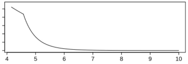
Figure 2: Density of the NHPP with changepoint at 4.57 (distribution (a)).
expected information for a single observation of 1/θ2 and 1/η2. Form
i observations on ¯Ri we thus use total
information ofmi/θˆi2or mi/ηˆi2, which is also an estimate ofm1P(X∈R¯i|X ∈R¯1)/θ2 (cf. Section 2.2), and
similarly forη.
3.2.2 Univariate case: ξ
We simulated 200 datasets of size / expected size 5000 according to the following distributions:
(a) NHPP on (4.15,∞) with a changepoint in intensity at 4.57;
(b) NHPP on (4.27,∞) with no changepoint (true parametersµ= 10, σ= 1, ξ= 0.1);
(c) Truncated (at zero) standard normal (theoreticalξ= 0);
(d) Truncated (at zero)tν-distribution, withν = 3 degrees of freedom (theoreticalξ= 1/3).
In case (a) there were an expected number of 2500 points either side of the changepoint at 4.57; parameters (µ, σ, ξ) changed from (21.4,1.4,−0.05) below the changepoint, to (10,1,0.1) above the changepoint, with the intensity constrained to be continuous at the change; the density of this is plotted in Figure 2. We apply the likelihood ratio (LR) testing procedure to the datasets to assess the quality of the inference when
using this to automatically select a threshold. In each case, there werek= 25 estimates considered ranging
from the 0 to 96% quantiles. For comparison we also consider the method of Northrop and Coleman (2014) (denoted NC), taking as the selection criterion “the lowest threshold above which the p-value is larger than 0.05 and remains larger than 0.05 at all higher thresholds”. If no threshold satisfied this rule then the highest threshold was used.
Table 2 details summaries of (i) the distribution of thresholds selected by the two methods, with
signif-icance level α= 0.05; (ii) the distribution and accuracy (as measured by root mean squared error, RMSE)
of the estimates of ξ; and (iii) the accuracy of the estimates of three high quantiles, or return levels, as
For all distributions the proposed method yields an improvement in RMSE. For case (a), the threshold at which the changepoint occurs is 4.57, thus the mean threshold taken by the LR test, at 4.51, is slightly too
low, and leads to a small negative bias in the estimation ofξ. However, the range of thresholds selected is
quite narrow, suggesting that the change is being identified. The mean threshold taken by the NC method is slightly too high and there is more variability in the selection, leading to worse overall performance. A similar comment applies to the thresholds selected for (b). For the LR method the lowest threshold was selected
89.5% of the time (i.e., 10.5% of the p-values were less than 0.05), whilst for the NC method the lowest
threshold was selected 69% of the time. This is due to the way this procedure is calibrated, as discussed in Section 3.1.1. For (c) and (d), the LR procedure tends to select slightly higher thresholds leading to smaller bias.
Threshold Shape Parameter Return Level RMSE
Mean Q0.05 Q0.5 Q0.95 Mean Q0.05 Q0.5 Q0.95 RMSE RL1 RL2 RL3
LR-(a) 4.51 4.42 4.51 4.60 0.09 0.05 0.09 0.14 0.03 0.99 1.87 3.21 NC-(a) 4.65 4.38 4.48 5.81 0.08 0.02 0.08 0.14 0.05 1.52 3.37 7.00 LR-(b) 4.31 4.27 4.27 4.31 0.09 0.07 0.10 0.12 0.04 0.88 1.61 2.69 NC-(b) 4.54 4.27 4.27 5.86 0.10 0.02 0.10 0.16 0.05 1.37 3.10 6.47 LR-(c) 1.10 0.52 1.01 2.06 -0.15 -0.22 -0.16 -0.02 0.16 0.41 0.67 0.95 NC-(c) 0.96 0.41 0.85 2.00 -0.17 -0.24 -0.18 -0.06 0.18 0.46 0.73 1.02 LR-(d) 1.21 0.51 1.11 2.20 0.25 0.14 0.24 0.38 0.12 20.01 68.91 228.06 NC-(d) 1.26 0.46 0.94 3.43 0.23 0.14 0.21 0.41 0.14 22.03 73.52 234.74
Table 2: Summaries of the thresholds and parameter estimates from the simulations. Qa stands for the
100a% quantile; RL1–RL3 correspond respectively to the 0.9, 0.99, and 0.999 quantiles of the distribution of
the maximum point in the set of observations. LR-(a) denotes the LR method used on distribution (a), etc.
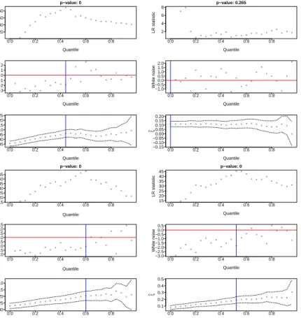
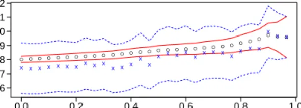
Example diagnostic plots are displayed in Figure 3; each is composed of three vertically stacked plots. The
uppermost of the three plots gives the values of the log-likelihood ratio 2{logL( ˆβj,γˆj, j)−logL(0,1,0)} ≥0
versus threshold, on a quantile scale. This is maximized injat the same point asL( ˆβj,ˆγj, j), and the value
at the maximum is equal to 2 logT, as defined in (9). The title of this plot displays the p-value associated
to T. The central plot is of the white noise process, with a horizontal line at 0, whilst the lower plot is
the traditional parameter stability plot with pointwise approximate 95% CIs. The selected thresholds are displayed by vertical lines on the central and lower plots. The likelihood ratio procedure can be seen to generally select a threshold where there are too many positive / negative points in the white noise process to the left of the threshold, and much more plausible white noise values to the right of the threshold. Of course, if preferred one could simply use these plots as a more informative and more interpretable version of the existing parameter stability diagnostic plot.
● ● ● ● ● ● ●● ● ● ● ●● ● ● ●●● ●●●● ● 0.0 0.2 0.4 0.6 0.8 20 30 40 50 p−value: 0 Quantile LR statistic ● ● ● ● ● ● ● ● ● ● ● ● ● ● ● ●● ● ● ● ● ● ● ● 0.0 0.2 0.4 0.6 0.8 −3 −2 −1 0 1 2 Quantile White noise ●●● ●●●● ●●●● ●● ●● ●● ●●● ●●●● ● 0.0 0.2 0.4 0.6 0.8 −0.05 0.00 0.05 0.10 0.15 0.20 0.25 Quantile ξ ^ ● ● ● ● ● ● ● ● ● ● ● ●●● ● ● ● ● ● ● ● ● ● 0.0 0.2 0.4 0.6 0.8 2 4 6 8 p−value: 0.265 Quantile LR statistic ● ● ● ● ● ● ● ●● ● ● ● ● ●● ● ● ● ● ● ● ● ● ● 0.0 0.2 0.4 0.6 0.8 −1.0 −0.50.0 0.5 1.0 1.5 2.0 Quantile White noise ●●●● ●●●● ●●●●● ●●●● ● ●●● ● ● ● ● 0.0 0.2 0.4 0.6 0.8 −0.15 −0.10 −0.050.00 0.05 0.10 0.15 0.20 Quantile ξ ^ ● ● ● ● ● ● ●● ● ● ● ● ● ● ●● ●● ● ● ● ● ● 0.0 0.2 0.4 0.6 0.8 15 20 25 30 35 40 45 p−value: 0 Quantile LR statistic ●● ●● ● ● ● ● ● ● ● ● ●● ● ● ● ● ● ● ● ● ● ● 0.0 0.2 0.4 0.6 0.8 −2.0 −1.5 −1.0 −0.50.0 0.5 1.0 1.5 Quantile White noise ●●● ●●●● ●●●● ●●●● ●●●●● ● ● ● ● ● 0.0 0.2 0.4 0.6 0.8 −0.30 −0.25 −0.20 −0.15 −0.10 Quantile ξ ^ ● ● ● ● ● ● ●● ● ●● ●● ● ● ●● ● ● ● ●●● 0.0 0.2 0.4 0.6 0.8 15 20 25 30 35 40 45 p−value: 0 Quantile LR statistic ● ● ● ● ● ● ● ● ● ● ● ● ● ● ● ● ● ● ● ● ● ● ● ● 0.0 0.2 0.4 0.6 0.8 −3.0 −2.5 −2.0 −1.5 −1.0 −0.50.0 0.5 Quantile White noise ●●●● ●●●● ●●●●● ●●●● ●●●● ●●● ● 0.0 0.2 0.4 0.6 0.8 0.1 0.2 0.3 0.4 0.5 Quantile ξ ^
Figure 3: Example diagnostic plots for dataset (a) (top left); (b) (top right); (c) (bottom left); (d) (bottom
right). The top panel in each plot shows the 2{logL( ˆβj,γˆj, j)−logL(0,1,0)} versus threshold; the central
3.2.3 Bivariate case: η
For estimation ofη, we simulated 200 datasets of size 5000 from the following dependence structures; for (b)
and (c), marginal distributions were transformed to be standard exponential via the empirical probability integral transform:
(a) Independence (theoreticalη= 0.5)
(b) Bivariate normal with dependence parameterρ= 0.8 (theoretical η= 0.9)
(c) Bivariatetν-distribution, with dependence parameterρ= 0.8 andν = 2 degrees of freedom (theoretical
η= 1)
Owing to the investigations in Section 3.1 that suggest the asymptotic multivariate normal distribution generally holds better for the rate parameterization of the exponential distribution, we use this for the
simulation study, transforming to η by exploiting equivariance of MLEs. Table 3 provides details of the
distribution of thresholds selected by the likelihood ratio test rule with α= 0.05, along with summaries of
parameter estimates, end estimates of probabilities of lying in extreme sets. These probabilities are calculated by exploiting the relation
P{(XE, YE)∈c+t+A} ∼e−c/ηP{(XE, YE)∈t+A}, c >0, t→ ∞,
for A ⊂ (0,∞)2, with addition applied componentwise. The set A0 = t+A is taken to be such that
P{(XE, YE) ∈ A0} can be estimated empirically. For case (a), min(XE, YE) is exactly exponential, but
for (b) and (c), the quality of the approximation depends on the rate convergence of the ratio of slowly-varying functions in equation (2) to unity. For reference, values obtained by taking the threshold as the 90% quantile are also included. The method of Northrop and Coleman (2014) is not directly applicable here as their model assumes multiple shape parameters, whereas here it is a change in exponential rate parameter that is being sought. One could develop a procedure in the spirit of their idea for these purposes, but we do not consider this further here.
In case (a), where the data are exactly exponential, the RMSEs are smaller for the thresholds selected by the LR rule, since the test is well calibrated and hence the lowest possible threshold is usually selected (in this case 94.5% of the time); this is reflected in the quantiles of the threshold distribution. Both dependence
structures (b) and (c) exhibit fairly slow rates of convergence, inducing bias in estimation ofη, though the
problem is worse for the bivariate normal. This bias is still present at the 90% quantile, but RMSEs are typically larger for the LR method with the extra uncertainty of the threshold incorporated.
Threshold Inverse Rate Parameter Probabilities
Mean Q0.05 Q0.5 Q0.95 Mean Q0.05 Q0.5 Q0.95 RMSE p1 p2 p3
LR-(a) 0.01 0.00 0.00 0.04 0.50 0.49 0.50 0.51 0.01 0.23 0.25 0.20 90%-(a) 0.50 0.47 0.50 0.53 0.02 0.46 0.48 0.41 LR-(b) 0.46 0.05 0.32 1.41 0.81 0.78 0.81 0.86 0.09 0.21 0.33 1.77 90%-(b) 0.84 0.80 0.84 0.88 0.06 0.24 0.17 1.57 LR-(c) 1.41 0.86 1.26 2.66 0.94 0.89 0.93 1.00 0.07 0.27 0.32 0.43 90%-(c) 0.95 0.91 0.96 0.99 0.05 0.17 0.21 0.34
Table 3: Summaries of the thresholds and estimates of η from the simulations. Columns labelled p1–p3
give the MSEs of all log probabilities of the pair (in standard exponential margins) lying in extreme sets
(7,8)×(7,8),(6.5,7.5)×(7.5,8.5),(5.5,6.5)×(8,9), respectively. LR-(a) denotes the LR method used on
distribution (a), etc.
●●●● ● ●● ● ● ● ● ● ● ●● ● ● ● ● ● ● ● ● 0.0 0.2 0.4 0.6 0.8 0 1 2 3 4 5 p−value: 0.529 Quantile LR statistic ● ●● ● ● ● ● ● ● ● ● ● ● ● ● ● ● ● ● ●● ● ●● 0.0 0.2 0.4 0.6 0.8 −1.5 −1.0 −0.5 0.0 0.5 1.0 1.5 Quantile White noise ●● ●●●● ●●●● ●●●●● ●●●● ●●●● ● ● 0.0 0.2 0.4 0.6 0.8 0.40 0.45 0.50 0.55 Quantile η ^ ● ● ● ● ● ● ● ●● ● ● ● ● ● ● ● ● ● ● ● ●●● 0.0 0.2 0.4 0.6 0.8 10 15 20 25 p−value: 0 Quantile LR statistic ● ● ● ● ●● ● ●● ● ● ● ●● ● ● ●● ● ● ● ● ● ● 0.0 0.2 0.4 0.6 0.8 −2.0 −1.5 −1.0 −0.5 0.0 0.5 Quantile White noise ●●● ●●●●● ●●●● ●●●● ●●●● ● ● ●●● 0.0 0.2 0.4 0.6 0.8 0.75 0.80 0.85 0.90 0.95 Quantile η ^ ●● ● ● ●● ● ● ● ●● ●● ●● ● ●● ●● ●● ● 0.0 0.2 0.4 0.6 0.8 10 15 20 25 30 35 40 p−value: 0 Quantile LR statistic ● ● ● ● ● ● ● ● ● ●● ● ● ● ● ● ● ● ● ● ● ● ● ● 0.0 0.2 0.4 0.6 0.8 −2.0 −1.5 −1.0 −0.5 0.0 Quantile White noise ● ●●●● ●●●● ●●●● ●●●●● ●●●● ●● ● 0.0 0.2 0.4 0.6 0.8 0.80 0.85 0.90 0.95 1.00 1.05 Quantile η ^
Figure 4: Diagnostic plots for the inverse rate parameterη, for dependence structures: (a) (left), (b) (centre)
and (c) (right).
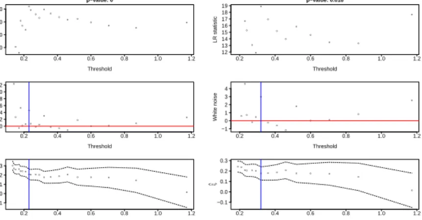
Example threshold diagnostic plots based on the exponential inverse rate parameter, η, are provided in
Figure 4, with the same interpretation as described in Section 3.2.2 for Figure 3. Figure 5 shows an example
plot based on the idea of independent estimators ˜ηoutlined in Section 2.3.2, for the same data as in the
right-hand panel of Figure 4. The confidence intervals in Figure 5 become slightly wider as the quantile decreases
for two reasons: (i) the uncertainty in ˜ηj does not decrease much for smallerj, in contrast with that for ˆηj;
(ii) the confidence intervals are calibrated such that each hypothesis test of the form “H0(j):ηi =η0 for all
i≥j” has a size of 0.05, thus increasingly large normal quantiles are used moving from right to left. Due
to the size of the confidence intervals, plots of this form do not seem to add much to the suite of threshold diagnostics, and this is why we have not pursued this line further.
4
Applications
Here we consider the use of the diagnostic plots from Figures 3 and 4 on some freely-available data. Code to produce these plots, written in R (R Core Team, 2014), is available online as detailed in Section 1.
● ● ● ● ● ● ● ● ● ● ● ● ● ● ● ● ● ●● ● ● ● ● ● ● ● ● ● ● ● 0.0 0.2 0.4 0.6 0.8 1.0 0.6 0.7 0.8 0.9 1.0 1.1 1.2 Quantile η ^ x x x x x x x x x x x x x x x x x x x x xx x x x x x x x x
Figure 5: Alternative diagnostic plot based on the independent estimators of Section 2.3.2.
4.1
Share Price Data
The R package evir (Pfaff and McNeil, 2012) contains data on daily log returns of the share prices of BMW and Siemens from January 1973 until July 1996. Returns such as these typically exhibit periods of volatility, which can often be dealt with by fitting a GARCH model to the data and using the standardized residuals. For these data we applied a GARCH(1,1) model, as is common in the literature (e.g. Hilal et al., 2011); the resulting standardized log returns appear much closer to stationarity. The marginal diagnostic plots for the positive returns are displayed in the leftmost two panels of Figure 6. In each case the lowest threshold considered in the plot was chosen as the lowest point above which the density appeared to be decreasing,
by an inspection of the histogram of the data. The number of thresholds used wask = 20. In the case of
the BMW data, the likelihood (8) for the threshold is maximized at roughly 1.47 (94% quantile), and the evidence against white noise is significant at the 5% level. For the Siemens data, the likelihood is maximized around 1.27 (91% quantile), and the evidence to reject a null hypothesis of white noise is even stronger.
The right-hand plot of Figure 6 displays the diagnostic for the coefficient of tail dependence between these two variables. To produce this plot, any days on which the returns are given as exactly zero for either BMW or Siemens were removed, and the remaining data were transformed to be marginally standard exponential
using the empirical probability integral transform. All remaining data were used, and thus we tookk= 30
thresholds. At the selected threshold, the estimated value ofη of about 0.72 (standard error 0.01) suggests
that these data are positively dependent in the extremes, but asymptotically independent.
4.2
Fort Collins Precipitation Data
The Fort Collins precipitation dataset, available in the R package extRemes (Gilleland and Katz, 2011), consists of daily measurements of precipitation, in inches, over a 100 year period. The data were analyzed by Katz et al. (2002); Scarrott and MacDonald (2012) also considered these data as an illustration of the difficulty of threshold selection. Although these data are available to the nearest 0.01 inch, there are many less extreme measurements which take the same value and cause the data to appear discrete in the body
●● ●● ●● ●● ● ● ● ● ● ● ● ● ● ● 0.5 1.0 1.5 2.0 4 6 8 10 12 14 p−value: 0.037 Threshold LR statistic ● ● ●● ● ● ● ● ● ● ● ● ● ● ● ● ● ● ● 0.5 1.0 1.5 2.0 −2 −1 0 1 2 3 Threshold White noise ●●●●●●●●●● ● ● ● ● ● ● ● ● ● ● 0.5 1.0 1.5 2.0 0.0 0.1 0.2 0.3 Threshold ξ ^ ● ● ● ● ● ● ● ● ● ● ● ● ● ● ● ● ● ● 0.5 1.0 1.5 2.0 10 15 20 25 30 35 p−value: 0 Threshold LR statistic ● ● ● ● ●● ● ● ● ● ● ● ● ● ● ● ● ● ● 0.5 1.0 1.5 2.0 −1.5 −1.0 −0.5 0.0 Threshold White noise ●●●●●●●●●● ● ● ● ● ● ● ● ● ● ● 0.5 1.0 1.5 2.0 −0.1 0.0 0.1 0.2 0.3 0.4 Threshold ξ ^ ● ●● ● ● ●● ● ●●● ●●● ●● ● ● ● ● ● ● ● ● ● ● ● ● 0.0 0.5 1.0 1.5 2.0 2.5 5 10 15 20 p−value: 0.011 Threshold LR statistic ● ● ● ● ● ● ● ● ● ● ● ●● ● ● ● ● ●● ● ● ● ● ● ● ● ● ● ● 0.0 0.5 1.0 1.5 2.0 2.5 −2 −1 0 1 2 Threshold White noise ●● ●● ●● ● ●● ● ● ● ● ● ●●●●●● ● ● ● ● ● ● ● ● ● ● 0.0 0.5 1.0 1.5 2.0 2.5 0.65 0.70 0.75 0.80 Threshold η ^
Figure 6: Marginal diagnostic plots for BMW standardized returns (left) and Siemens standardized returns (centre). Diagnostic plot for the coefficient of tail dependence (right).
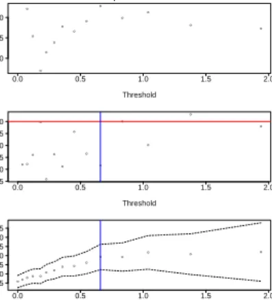
and lower tail in particular. The left-hand plot in Figure 7 shows data considered above the 0.64 quantile of positive values, where there are 197 unique values out of 2916; the right-hand plot shows data above the 0.72
quantile of positive values, where there are 191 unique values out of 2171. We used k= 20 thresholds for
the left-hand plot, and the upper 15 of those thresholds for the right-hand one. In the first case the selected threshold is 0.23 inches, lower than the 0.4 inches taken by Katz et al. (2002), but the shape parameter
estimate of ˆξ = 0.21 (standard error 0.03) is consistent with their estimate of 0.18. In the second case,
the selected threshold is 0.32 inches, and the estimate ˆξ= 0.18 (standard error 0.03) is consistent with the
others. The likelihood (8) increases again at the highest threshold of roughly 1.2, and indeed Scarrott and MacDonald (2012) also identified 1.2 inches as a candidate threshold. We discuss repeated application of the test in Section 5.
● ● ● ● ● ● ● ● ● ● ● ● ● ● ● ● ● ● 0.2 0.4 0.6 0.8 1.0 1.2 150 160 170 180 p−value: 0 Threshold LR statistic ● ● ● ● ●● ● ● ●● ● ● ● ● ● ● ● ● ● 0.2 0.4 0.6 0.8 1.0 1.2 0 2 4 6 8 10 12 Threshold White noise ● ●●● ● ●● ● ●●● ● ● ● ● ● ● ● ● ● 0.2 0.4 0.6 0.8 1.0 1.2 −0.1 0.0 0.1 0.2 0.3 Threshold ξ ^ ● ● ● ● ● ● ● ● ● ● ● ● ● 0.2 0.4 0.6 0.8 1.0 1.2 12 13 14 15 16 17 18 19 p−value: 0.018 Threshold LR statistic ● ● ● ● ● ● ● ● ● ● ● ● ● ● 0.2 0.4 0.6 0.8 1.0 1.2 −1 0 1 2 3 4 Threshold White noise ●● ● ●●● ● ● ● ● ● ● ● ● ● 0.2 0.4 0.6 0.8 1.0 1.2 −0.1 0.0 0.1 0.2 0.3 Threshold ξ ^
4.3
Loss-ALAE Data
Data on the indemnity payments (Loss) and allocated loss adjustment expense (ALAE) relating to 1500 general liability claims from insurance companies are available in the R package evd (Stephenson, 2002). The data were transformed to have standard exponential margins by the empirical probability integral transform, and we concern ourselves only with the estimation of their extremal dependence structure. Figure 8 displays
the diagnostic plots for dependence threshold assessment, with k = 15 thresholds used. At the selected
threshold, the MLE ˆη = 0.79 (standard error 0.035), indicates moderately strong positive dependence, but
asymptotic independence of the pair. However, as pointed out by Beirlant et al. (2004, p.351) the uncertainty
in assessment of η is most likely underestimated by procedures such as this one, which do not account for
the uncertainty of the marginal transformations.
● ● ● ● ● ● ● ● ● ● ● ● ● 0.0 0.5 1.0 1.5 2.0 10 15 20 p−value: 0.004 Threshold LR statistic ●● ● ● ● ● ● ● ● ● ● ● ● ● 0.0 0.5 1.0 1.5 2.0 −2.5 −2.0 −1.5 −1.0 −0.5 0.0 Threshold White noise ●●●●●●●● ● ● ● ● ● ● ● 0.0 0.5 1.0 1.5 2.0 0.65 0.70 0.75 0.80 0.85 0.90 0.95 Threshold η ^
Figure 8: Dependence threshold diagnostics for the Loss-ALAE data.
5
Discussion
We have advocated the use of the asymptotic joint distribution of MLEs to offer a more interpretable threshold diagnostic plot. Based on the properties of this joint distribution we also suggested a likelihood-based method for selecting a threshold, with significance assessed by simulation; performance has been assessed on both simulated data, and a variety of different measured datasets. As has been widely observed in the literature, there is rarely an obvious choice for a threshold, and methods to account for the uncertainty in threshold estimation (see e.g. MacDonald et al., 2011; Wadsworth and Tawn, 2012; Scarrott and MacDonald,
2012, and references therein), are clearly important in dealing with this. However, each such piece of
methodology naturally comes with advantages and disadvantages, with none representing a panacea for the problem. As such, common applied practice remains to use fixed thresholds chosen via threshold diagnostic
plots. The ideas proposed in this article are intended to augment this “simple” end of the threshold selection technique spectrum.
Although formulation of the white noise process ξ∗ requires no more fits or assumptions than the
for-mulation of a parameter stability plot, it can be the case that the estimated joint covariance matrix for ( ˆξ1, . . . ,ξˆk)T is not always positive definite. This has not proved to be a big problem for simulated data, but
is more of an issue for measured data. One issue with environmental data in particular is rounding, such that, particularly for less extreme values, data appear discrete. The correct way to overcome this is to use a multinomial likelihood, as the true measurement could lie anywhere within the rounding limits. We have not considered this, but have noted that adding uniform noise within rounding limits tends to produce much better performance, so that such issues do seem largely attributable to the rounding. It is also noteworthy that the ideas in this paper rely on asymptotic results for the joint distribution of MLEs, and, as suggested by Table 1, may not prove useful in small samples.
We have not considered the multiple testing aspects of applying the likelihood ratio test sequentially, but one could investigate this in principle. Informally, we comment that in the Fort Collins example of Section 4.2, considering only data above 0.74 (the 95% threshold) there appears to be some evidence that a higher threshold is to be preferred, but there is some sensitivity to the number of thresholds taken. The values of the white noise process will naturally differ when different candidate thresholds are considered, and
thus may sometimes suggest different selected thresholdsu∗. This is a disadvantage not just of the proposed
method, but fixed threshold selection in general, and often an uncomfortable feature of real data. Methods for incorporating threshold uncertainty are necessary to cope with this. The plots that we advocate here do at least help to elucidate the features of the data in this respect.
Whilst we have focussed on the white noise process for the shape parameterξ∗, equation (6) suggests that
we could have combined information from all three parameters (µ, σ, ξ) across thresholds. We investigated
this, but found that in general the 3×3 covariance matrixIi+1−1 −Ii−1is rarely estimated as positive-definite.
As mentioned in an asymptotic context in Section 2, one can consider the NHPP as a superposition of a number of Poisson processes, and one can in fact select a number arbitrarily for convenience. If this is chosen
as, say,N, then the estimated parameters (µ, σ, ξ) correspond to the parameters for the GEV distribution
for block maxima over N blocks (e.g. Coles, 2001, p.133). The relationship between this tuning parameter
and the number of threshold exceedances has a substantial effect on the correlations between (ˆµ,σ,ˆ ξˆ) (e.g.
Acknowledgements
I am grateful to a referee and associate editor for constructive comments that have improved the paper.
References
Beirlant, J., Dierckx, G., Goegebeur, Y., and Matthys, G. (1999). Tail index estimation and an exponential
regression model. Extremes, 2(2):177–200.
Beirlant, J., Goegebeur, Y., Segers, J., and Teugels, J. (2004). Statistics of Extremes. Wiley.
Coles, S. G. (2001).An Introduction to the Statistical Modeling of Extreme Values. Springer-Verlag, London.
Cook, T. D. and DeMets, D. L. (2008). Introduction to Statistical Methods for Clinical Trials. Chapman &
Hall / CRC.
Davison, A. C. and Smith, R. L. (1990). Models for exceedances over high thresholds (with discussion).
Journal of the Royal Statistical Society. Series B (Methodological), 52(3):393–442.
Eckley, I. A., Fearnhead, P., and Killick, R. (2011). Analysis of changepoint models. In Barber, D., Cemgil,
A. T., and Chiappa, S., editors,Bayesian Time Series Models. Cambridge University Press, Cambridge.
Ferreira, A., de Haan, L., and Peng, L. (2003). On optimising the estimation of high quantiles of a probability
distribution. Statistics, 37(5):401–434.
Gilleland, E. and Katz, R. W. (2011). New software to analyze how extremes change over time. Eos,
92(2):13–14.
Gomes, M. I. (1994). Penultimate behaviour of the extremes. In Galambos, J., Lechner, J., and Simiu, E.,
editors,Extreme Value Theory and Applications, Volume 1. Kluwer Academic Publishers.
Hilal, S., Poon, S.-H., and Tawn, J. A. (2011). Hedging the black swan: Conditional heteroscedasticity and
tail dependence in S&P500 and VIX. Journal of Banking and Finance, 35:2374–2387.
Katz, R. W., Parlange, M. B., and Naveau, P. (2002). Statistics of extremes in hydrology. Advances in
Water Resources, 25:1287–1304.
Leadbetter, M. R., Lindgren, G., and Rootz´en, H. (1983). Extremes and Related Properties of Random
Ledford, A. W. and Tawn, J. A. (1996). Statistics for near independence in multivariate extreme values.
Biometrika, 83(1):169–187.
Lee, J., Fan, Y., and Sisson, S. A. (2013). Bayesian threshold selection for extremal models using measures
of surprise. http://http://arxiv.org/abs/1311.2994.
MacDonald, A., Scarrott, C., Lee, D., Darlow, B., Reale, M., and Russell, G. (2011). A flexible extreme
value mixture model. Computational Statistics and Data Analysis, 55(6):2137–2157.
Northrop, P. J. and Coleman, C. L. (2014). Improved threshold diagnostic plots for extreme value analyses.
Extremes, 17(2):289–303.
Pfaff, B. and McNeil, A. (2012). evir: Extreme Values in R. R package version 1.7-3.
Pickands, J. (1971). The two-dimensional Poisson process and extremal processes. Journal of Applied
Probability, 8(4):745–756.
Pickands, J. (1975). Statistical inference using extreme order statistics. Annals of Statistics, 3:119–131.
R Core Team (2014).R: A Language and Environment for Statistical Computing. R Foundation for Statistical
Computing, Vienna, Austria.
Scarrott, C. and MacDonald, A. (2012). A review of extreme value threshold estimation and uncertainty
quantification. Revstat, 10(1):33–60.
Siegmund, D. (1985). Sequential Analysis: Tests and Confidence Intervals. Springer-Verlag, New York.
Smith, R. (1985). Maximum likelihood estimation in a class of nonregular cases. Biometrika, 72(1):67–90.
Smith, R. L. (1987). Approximations in extreme value theory. University of North Carolina, Department of Statistics, Technical Report No. 205.
Stephenson, A. G. (2002). evd: Extreme value distributions. R News, 2(2):31–32.
Wadsworth, J. L. and Tawn, J. A. (2012). Likelihood-based procedures for threshold diagnostics and
uncer-tainty in extreme value modelling. Journal of the Royal Statistical Society: Series B, 74(3):543–567.
Wadsworth, J. L., Tawn, J. A., and Jonathan, P. (2010). Accounting for choice of measurement scale in
extreme value modeling. Annals of Applied Statistics, 4(3):1558–1578.
Supplementary Material to
Exploiting structure of maximum
likelihood estimators for extreme value threshold selection
J. L. Wadsworth
Statistical Laboratory, University of Cambridge, U.K.
December 1, 2014
A
Derivation of joint distribution of MLEs
A.1
Poisson Process Likelihood
Consider a Poisson process on a space X, with intensityλθ(x), and denote the integrated intensity over a region
R, by Λθ(R) = R
Rλθ(x)dx. The likelihood function for a sample (X1, . . . , XN, N), with (X1, . . . , XN) observed on R, is given in (3). DefineR1, . . . , Rk and ¯R1, . . . ,R¯k as in Section 2. Then we can equally write the likelihood (3)
as LR(θ) = ( Y i:xi∈R1 λθ(xi) ) exp{−Λθ(R1)} × · · · × ( Y i:xi∈Rk λθ(xi) ) exp{−Λθ(Rk)}, since Λθ(R) =P k
i=1Λθ(Ri). The array of likelihoods forθ on ¯R1, . . . ,R¯k is
LR¯1(θ) = ( Q i:xi∈R1 λθ(xi) ) e−Λθ(R1) × ( Q i:xi∈R2 λθ(xi) ) e−Λθ(R2) × · · · × ( Q i:xi∈Rk λθ(xi) ) e−Λθ(Rk) LR¯2(θ) = ( Q i:xi∈R2 λθ(xi) ) e−Λθ(R2) × · · · × ( Q i:xi∈Rk λθ(xi) ) e−Λθ(Rk) · · · · LR¯k(θ) = ( Q i:xi∈Rk λθ(xi) ) e−Λθ(Rk).
To consider asymptotic behaviour, we suppose that the data arise frommsuperpositions of such Poisson processes. Let ˆθ1, . . . ,θˆk be the MLEs from LR¯1, . . . , LR¯k, respectively. Denoting the log-likelihoods by`R¯1, . . . , `R¯k, which we now suppose to be functions of the random data, we can write
asm→ ∞, giving the usual asymptotic normal distribution,N(0, Ij−1), forj= 1, . . . , k, andIj :=E{−∇2`R¯j(θ0)}, expectation being both over the number of points on ¯Rj for a single Poisson process, and their locations on ¯Rj.
By the properties of the Poisson process, the data Xi and numbersNj on each region are mutually independent,
and from the above, we observe that we can write each∇`R¯j(θ0) as a sum of independent contributions
∇`R¯j(θ0) =
k
X
i=j
∇`Ri(θ0).
Using the fact that{−∇2` ¯ Rj( ˆθj)/m} −1=E{−∇2` ¯ Rj(θ0)} −1+o p(1), we have m1/2( ˆθ1−θ0) =I1−1m −1/2 k X i=1 ∇`Ri(θ0) +op(1) m1/2( ˆθ2−θ0) =I2−1m −1/2 k X i=2 ∇`Ri(θ0) +op(1) · · · m1/2( ˆθk−θ0) =Ik−1m −1/2 ∇`Rk(θ0) +op(1).
Asm→ ∞, the above array converges in distribution to
T1 T2 .. . Tk = I1−1 {Z1 + Z2 + · · · + Zk} I2−1 {Z2 + · · · + Zk} .. . . .. ... Ik−1 Zk = Diag1≤i≤k(Ii−1) 1p 1p · · · 1p 0 1p · · · 1p .. . . .. ... 0 0 · · · 1p Z1 Z2 .. . Zk ,
with 1p thep-dimensional identity matrix, andZj∼N(0, IRj) independent forj= 1, . . . , k. Noting that
Cov 1p 1p · · · 1p 0 1p · · · 1p .. . . .. ... 0 0 · · · 1p Z1 Z2 .. . Zk ={Imax(i,j)}1≤i≤k,1≤j≤k,
one can easily verify that the covariance matrix of (T1, . . . ,Tk)T is equal to ({I−1}min(i,j))1≤i≤k,1≤j≤k.
A.2
Likelihood with nonrandom number of points
We now suppose that there is a nonrandom total ofm1 observations on ¯R1, and without loss of generality,P(X ∈ ¯
·)/P(X ∈ R¯j) etc., be the density and probability measure normalized over ¯Rj. Dependence of the probability
measure onθ is made implicit. We consider likelihoods of the form
LR¯j(θ) = m1 Y i=1 fR¯j(xi;θ) 1(Xi∈R¯j)= Y i:xi∈R¯j fR¯j(xi;θ).
As in Section A.1, let `R¯
j(θ) = logLR¯j(θ), and let`
(1) ¯
Rj(θ) be a single component of the sum. In Section A.1, we used k-dimensional arrays for exposition. However, we could have noted that the concatenated vector of scores
(∇`R¯1(θ0), . . . ,∇`R¯k(θ0))T (A.1)
is a sum of mean-0iid random vectors, and thus as long as the covariance matrix of the iid components of the sum,Cov{(∇`(1)R¯1(θ0), . . . ,∇`
(1) ¯
Rk(θ0))
T}= Σ has finite entries then a multivariate normal limit holds when (A.1) is
multiplied by m−11/2, m1 → ∞. The entries of the covariance matrix can be established by pairwise arguments, which is what we focus on here.
Consider two regions, say ¯Rj, ¯Rj+1, so that ¯Rj=Rj∪R¯j+1. Their indexing need not be consecutive, but will reduce clutter in notation. Then
1(Xi∈Rj)∼Bernoulli(P(X ∈Rj)), 1(Xi∈R¯j+1)∼Bernoulli(P(X ∈R¯j+1)). The likelihood for a single point on ¯Rj can be written
L(1)R¯j(θ) = ( fR¯j(xi;θ) PR¯j(X ∈Rj) )1(Xi∈Rj)( fR¯j(xi;θ) PR¯ j(X ∈ ¯ Rj+1) )1(Xi∈R¯j+1) PR¯j(X∈Rj) 1(Xi∈Rj)P ¯ Rj(X ∈ ¯ Rj+1)1(Xi∈ ¯ Rj+1), (A.2) and on ¯Rj+1 L(1)R¯ j+1(θ) =fR¯j+1(xi;θ) 1(Xi∈R¯j+1)= ( fR¯j(xi;θ) PR¯j(X ∈R¯j+1) )1(Xi∈R¯j+1) .
The score function for a single point on ¯Rj is
∇`(1)R¯j(θ) =∇` (1) Rj(θ) +∇` (1) ¯ Rj+1(θ) +1(Xi∈Rj) ∇PR¯j(X ∈Rj) PR¯j(X ∈Rj) +1(Xi∈R¯j+1) ∇PR¯j(X∈R¯j+1) PR¯j(X∈R¯j+1) , (A.3) with ∇`(1)R j(θ) = 1(Xi ∈Rj)∇fRj(X;θ)/fRj(X;θ). Noting that E{∇` (1) Rj(θ0)} =E{∇` (1) ¯ Rj+1(θ0)} = 0, and using
conditional expectation, Cov{∇`(1)R¯j+1(θ0),1(Xi∈R¯j+1)}=Cov{∇` (1) ¯ Rj+1(θ0),1(Xi∈Rj)}=Cov{∇` (1) ¯ Rj+1(θ0),∇` (1) Rj(θ0)}= 0,
so that∇`(1)R¯j+1(θ0) is uncorrelated with all components of∇` (1)
¯
Rj(θ0) except itself; i.e. Cov{∇`
(1) ¯ Rj+1(θ0),∇` (1) ¯ Rj(θ0)} =Var{∇`(1)R¯ j+1(θ0)}=P(X ∈ ¯ Rj)Ij, withIj=E{−∇2logfR¯ j(X;θ0)}.
By extension to any pair of indices,Cov{∇`(1)R¯
i(θ0),∇` (1) ¯ Rj(θ0)}=Var{∇` (1) ¯
Rmax(i,j)(θ0)}, so that normalizing the true scores by the square root of the expected number of points on the appropriate region gives the central limit convergence ∇`R¯1(θ0) m11/2P(X ∈R¯1)1/2 , . . . , ∇`R¯k(θ0) m11/2P(X∈R¯k)1/2 !T d →Npk(0,Ω), m1→ ∞, (A.4)
with Ω = {Imax(i,j)}1≤i≤k,1≤j≤k. The covariance matrix of the MLEs as opposed to the score follows as in
Sec-tion A.1.
In practice one may select ¯R1, . . . ,R¯k in order to fix a certain number of points m1, . . . , mk in each. In this
case the regions, rather than the number of points falling in each region, become random. At a practical level, with only a single sample, this does not alter the exploitation of the above results. At a theoretical level, expectations would change from being over random numbers to random regions.