Visualizing exploratory factor analysis models

(1)

SFB 649 Discussion Paper 2008-012

Visualizing exploratory

factor analysis models

Sigbert Klinke*

Cornelia Wagner*

* Humboldt-Universität zu Berlin, Germany

This research was supported by the Deutsche

Forschungsgemeinschaft through the SFB 649 "Economic Risk". http://sfb649.wiwi.hu-berlin.de

ISSN 1860-5664

SFB 649, Humboldt-Universität zu Berlin Spandauer Straße 1, D-10178 Berlin

S

FB

6

4

9 E

C

O

N

O

M

I

C

R

I

S

K

B

E

R

L

I

N

(2)

Visualizing exploratory factor analysis models

Sigbert Klinke1,2 _{and Cornelia Wagner}2

1 _{Institute for Statistics and Econometrics, School of Business and Economics,}

Humboldt-Universit¨at zu Berlin, Spandauer Strasse 1, 10178 Berlin, Germany, [email protected]

2

Department of Business education, Institute of Education, Faculty of Arts IV, Humboldt-Universit¨at zu Berlin, Unter den Linden 6, 10099 Berlin, Germany, [email protected]

Abstract. Exploratory factor analysis (EFA) is an important tool in data analyses, particularly in social science. Usually four steps are carried out which contain a large number of options. One important option is the number of factors and the association of variables with a factor. Our tools aim to visualize various models with different numbers in parallel of factors and to analyze which consequences a specific option has. We apply our method to data collected at the School of Business and Economics for evaluation of lectures by students. These data were analyzed by Zhou (2004) and Reichelt (2007).

Keywords: Factor analysis, visualization, questionnaire, evaluation of teach-ing

JEL classification:C39, C45, C63

1 Introduction

The exploratory factor analysis of a dataset consists of four steps:

1. estimating the correlation matrix Rˆ between the observed p items. The Bravais-Pearson correlation is the one usually used. For ordinal data

Kendall’sτb, Spearmans rank correlation or polychoric correlation

(un-derlying variable approach, see e.g. Bartholomew, Steele, Moustaki and Galbraith, 2002) can be used.

2. estimating the number of common factors k < p. Various criteria are used to find the number of factors: Kaiser (eigenvalues larger than 1), Parallel analysis of Horn (1965), 90% of explained variance and Elbow-criterion.

This work was supported by the Deutsche Forschungsgemeinschaft through the SFB 649 ”Economic risk” and the Multimedia-F¨orderprogramm 2006 of the Humboldt-Universit¨at zu Berlin.

(3)

2 Klinke, S. and Wagner, C.

3. estimating the loadings matrix Aˆ of the common factors. Depending on the beliefs about the data, several extraction methods can be used: principal component (PC), principal axis (PA), maximum likelihood (ML), unweighted least squares (ULS).

4. rotating the loadings to improve interpretability. Different rotation meth-ods have been developed, e.g. the varimax rotation if the rotated factors should be uncorrelated and the promax rotation if the rotated factors can be correlated.

2 Visualizations

We have used four plots to obtain information about our items and factor models:

correlation plot which visualizes the underlying correlation matrix of the items (see Figure 1 left). White here represents a small correlation whereas black represents a large absolute correlation. If we group the highly cor-related variables together then we can see which variables will become a factor.

scree plot which is a simple Scree plot added with the decision criteria (see Figure 1 right) mentioned before. The horizontal grey line represents the Kaiser criterion, the (nearly) horizontal falling line represent the Horn criterion and the vertical lines the 10%, ..., 90% variance criterion. This plot indicates how many factors should be chosen.

factor model plot we can see for each factor model which variables are explained by the same factor (see Figure 2). These variables are combined by a grey horizontal line. A grey square indicates that the absolute factor loading is smaller than a cut-off value (default: 0.5), but still has its absolute maximum loading at this factor. The black square indicates that the absolute factor loading is above the cut-off value. The colored plot version allows to differentiate between between small and large loadings above the cut-off value.

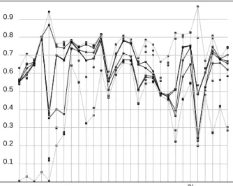
communality plot where each curve represents one factor model and shows how much ”variance” is explained by it (see Figure 3). For each model we can see where it improves the variance explanation of an item. In all graphics except the scree plot we can choose the order of the vari-ables. In the correlation plot the variables are arranged in such a way that variables with the largest absolute correlation are near to each other. In the factor model plot and communality plot we count, in all computed models,

how often variables are explained by the same factor (based on the greyand

black squares). The variables with the highest counts are placed near to each other.

(4)

Visualizing exploratory factor analysis models 3 b7 c9 f3 f1 c4 c3 c8 c1 c2 c5 c6 c7 b3 b2 b1 b4 b6_2 b6 b5 f4 f2 e3 e2 e1 e4 e5 d1 d3 d2 d2 d3 d1 e5 e4 e1 e2 e3 f2 f4 b5 b6 b6_2 b4 b1 b2 b3 c7 c6 c5 c2 c1 c8 c3 c4 f1 f3 c9 b7 Screeplot(s) Factor Explained variance 0.1 0.2 0.3 5 1 0 1 52 02 5 uv,uls,varimax Fi g. 1. Le ft : T e trac ho ric correl ati on of the 29 it e m s in the ev al uati on data. A dark er ci rcle m e a ns a hi gher a bs ol ute correlat ion b et w een the it e m s (whit e : b et w e en -0. 2 and 0.2, ... , blac k : b elo w -0. 8 or ab o v e 0. 8). Ri gh t: Sc re e pl ot for th e ev aluat ion dat a. The horiz on tal grey li ne indic ates the K ai se r c riteri on, the slo wly fall ing, nearly hori zon tal, grey li ne the H orn cri terio n and the v erti cal grey li ne s indic ate the 10%, 20% , .. . up to 90% ex pl ained v ari ance lines.

(5)

4 Klinke, S. and Wagner, C. uv,uls,varimax Variables Factor models 1 E%3 2 %4 3 %5 4 5 H%6 6 K 7 8 %7 9 10 e5 d2 d1 d3 e4 f1 f3 f4 e3 e1 e2 f2 b5 b4 b1 b2 b3 c2 c1 c4 c3 b7 b6 b6_2 c9 c8 c6 c5 c7

Fig. 2. We see the factor models starting from one up to ten factors. Black squares indicate an absolute loading larger than 0.5, grey squares indicate the largest ab-solute loading of a variable. Variables explained by the same common factor are connected by a grey line.

uv,uls,varimax Variables Communalities 0.1 0.2 0.3 0.4 0.5 0.6 0.7 0.8 0.9 e5 d2 d1 d3 e4 f1 f3 f4 e3 e1 e2 f2 b5 b4 b1 b2 b3 c2 c1 c4 c3 b7 b6 b6_2 c9 c8 c6 c5 c7

Fig. 3. Communalities of variables explained by several factor models. The lower grey line represents the one-factor model, the upper grey line the ten-factor model, the black lines the four-, five-, six- and seven-factor model (from lower to upper).

(6)

Visualizing exploratory factor analysis models 5

3 Application

For more than ten years, each semester students of the School of Business and Economics have been asked (see appendix A) to evaluate by questionnaire the lectures they have attended. Questionnaire data for the summer term 2002, 2003, 2005 and 2006 was analyzed by Zhou (2004) and Reichelt (2007). Here we reanalyze the data from lectures in the summer term of 2003 where the questionnaire consisted of 29 questions, each item with five answers ranging from good to bad. The missing values have been replaced by the maximum likelihood for categorical data method as described in Schafer (1997, p. 239ff). The correlation plot, Figure 1 left, indicates that we should expect around five factors. One with the variables e5-d3; this is pretty much uncorrelated with all other factors. The other four groups of variables (c4-c5, c6+c7, b3-b6, b5-e1) seem to be correlated to each other.

In the scree plot in Figure1 (right) we identify four (Horn) or five factors (Kaiser). Both explain between 60% and 70% of the total variance. Zhou (2004) identified five factors: ”communication skill” (b1, b2, b3, b4, c1, c2, c3), ”lecture notes” (c5, c6, c7), ”course attributes” (d1, d2, d3, e5), ”question answering” (b6, b6 2) and ”student reactions” (e1, e2, e3, f2, f4). It might also be interesting to look at the seven factor model since the eigenvalue curve here falls down a fraction.

For the factor model plot we therefore decided to visualize all models starting from a one factor model up to a ten factor model. We are currently looking for a set of variables which form a factor and which is stable to about several factor models.

Looking for the models, especially the four till seven factor model, we see that

• the variables e5, d1, d2 and d3 (course attributes) form a stable

fac-tor over nearly all models. Since the questionnaire was carried out four weeks before the exams, the student could also appreciate the speed and difficulties of a course.

• Another set of variables is f2, f4, e1, e2 and e3 (student reactions).

How-ever, as the variable f4 also loads on a different factor, it might be better to exclude it from the factor.

• c5, c6 and c7 also form a stable factor (lecture notes).

• In the eight factor model the variables b1-b5 and c1-c4 form one factor

(communications skill). However some variables turn out to be problem-atic in earlier models: b3 and b5 belong either to different factors or also load on a different factor.

• Finally, we have two factors (f1, f3 and ”question answering”: b6, b6 2,

b7) with a small number of items.

We end up with four or six factors depending whether we want factors with a small number of items or not. This complies with Zhou’s result (2004) that a six factor model is appropriate; her final choice of a five factor model is

(7)

6 Klinke, S. and Wagner, C.

visual analysis of several factor models provides us with a more informative

and reliable result.

However, an analysis of later data in Reichelt (2007) for the lectures in 2005

and 2006 revealed a high correlation (

≈

0 .

7) between the factors

”commu-nication skills” and ”lecture notes”. This is also reflected to some extent in

the factor models: later split of factors means higher correlation between the

factors, see for example the factor ”course attributes”. This clearly indicates

that students tend to make a general judgement about a lecture rather than

differentiating its characteristics which in Reichelt (2007) led to a two factor

model:

1. Did the student like the course?

2. Did the student consider the course difficult?

4 R routines

efa

//

efa

.

compute

//

((

P

B

efa

.

plotScree

efa

.

plotCorr

_prax

uls

horn

OO

efa

.

plotFactor

efa

.

computeCor

OO

efa

.

sortIndex

gg

NNNNN

_NNNNN

NNNNN

66 n

n

_//

efa

.

plotCommunality

Fig. 4.

Shows the relationship of the

efa

routines. The underlined routines are the

ones which are usually used.

To produce our plots we have written several R routines. Figures 4 and 5

show the order how the routines should be applied:

efa

generates from a data set a R object of class

efa

and computes a

cor-relation matrix. Possible corcor-relations are:

pearson

(default) for

Bravais-Pearson correlation,

kendall

for Kendalls

τ

,

spearman

for Spearmans

rank correlation,

cov

for covariance and

uv

for tetrachoric correlation

(slow).

efa.plotCorr

visualizes the correlation between the variables (see Figure 1

left).

Fig. 4. Shows the relationship of theefaroutines. The underlined routines are the ones which are usually used.

due to the fact that in the other three datasets she found a five-factor model. The visual analysis of several factor models provides us, via stability analysis and variance explanation for each item, with a more informative and reliable result.

However, an analysis of later data in Reichelt (2007) for the lectures in

2005 and 2006 revealed a high correlation (≈0.7) between the factors

”com-munication skills” and ”lecture notes” in a promax rotated model. This is also reflected to some extent in the factor models: later split between items means higher correlation between them, see for example the factor ”course attributes”. This clearly indicates that students tend to make a general judg-ment about a lecture rather than differentiating its characteristics which in Reichelt (2007) led to a two factor model:

1. Did the student like the course?

2. Did the student consider the course difficult?

4 R routines

To produce our plots we have written several R routines. Figures 4 and 5 show the order how the routines should be applied:

efa generates from a data set a R object of class efaand computes a

cor-relation matrix. Possible corcor-relations are:pearson(default) for

Bravais-Pearson correlation, kendall for Kendalls τ, spearman for Spearmans

rank correlation, cov for covariance and uv for tetrachoric correlation

(slow).

efa.plotCorr visualizes the correlation between the variables (see Figure 1 left).

(8)

Visualizing exploratory factor analysis modelsVisualizing exploratory factor analysis models 7 7 v l 0 3 _ f u l l < - r e a d . c s v 2 (" v l 0 3 _ i m p u t e . csv ") v l 0 3 < - v l 0 3 _ f u l l [ ,8:36] # e x t r a c t q u e s t i o n a n s w e r s e f a _ v l 0 3 < - efa ( vl03 , " uv ") efa . p l o t C o r r ( e f a _ v l 0 3 ) e f a _ v l 0 3 < - efa . c o m p u t e ( e f a _ v l 0 3 , f a c t o r s =10 , e x t r a c t =" uls " , h o r n = T ) efa . p l o t S c r e e ( e f a _ v l 0 3 ) efa . p l o t F a c t o r ( e f a _ v l 0 3 ) efa . p l o t C o m m u n a l i t y ( e f a _ v l 0 3 , m o d e l s e p = c (1 ,4:7 ,10) , col = c (" g r e y " , " b l a c k " , " b l a c k " , " b l a c k " , " b l a c k " , " g r e y "))

Fig. 5. Basic R program to generate the graphics in the paper.

efa.compute computes the factor models based on the correlation matrix.

Options are none, promax andvarimax (default) for rotation, pc

(prin-cipal component),uls(unweighted least squares),mle(maximum

likeli-hood) andpraxprincipal axis for extraction. The parameterfactors

de-termines the maximal number of factors and can either be a text (kaiser,

ellbow orhorn) or a number. Numbers between zero and one are inter-preted as minimal percentage of variance explained and numbers larger than one give the maximal number of factors to be extracted.

efa.plotFactors visualizes the computed factor models (see Figures 2),

efa.plotScree shows the scree plot with the selection criteria (see Figures 1 right) and

efa.plotCommunality shows the explained variance per item (see Figure 3). Additionally some helper routines have been written to realise specific ex-traction methods etc.:

uls unweighted least squares method to compute the factor loadings,

prax principal axis method to compute the factor loadings (like in SPSS),

horn computes the eigenvalues for a parallel analysis (Horn, 1965),

efa.computeCor computes the correlation for an R object of class efaand

efa.sortIndex computes an order of variables based on a square matrix, e.g. the correlation matrix.

The R routines are still in development, but can be requested from the first author ([email protected]).

5 Conclusion

The factor model plot, in particular, will simplify the task of understanding how many factors we can identify with an exploratory factor analysis and

Fig. 5. Basic R program to generate the graphics in the paper.

efa.compute computes the factor models based on the correlation matrix.

Options arenone, promax andvarimax(default) for rotation, pc

(prin-cipal component),uls(unweighted least squares),mle(maximum

likeli-hood) andpraxprincipal axis for extraction. The parameterfactors

de-termines the maximal number of factors and can either be a text (kaiser,

elbowor horn) or a number. Numbers between zero and one are inter-preted as minimal percentage of variance explained and numbers larger than one give the maximal number of factors to be extracted.

efa.plotFactors visualizes the computed factor models (see Figures 2),

efa.plotScree shows the scree plot with the selection criteria (see Figures 1 right) and

efa.plotCommunality shows the explained variance per item (see Figure 3). Additionally some helper routines have been written to realize specific extraction methods etc.:

uls unweighted least squares method to compute the factor loadings,

prax principal axis method to compute the factor loadings (like in SPSS),

horn computes the eigenvalues for a parallel analysis (Horn, 1965),

efa.computeCor computes the correlation for an R object of classefaand

efa.sortIndex computes an order of variables based on a square matrix, e.g. the correlation matrix.

The R routines are still in development, but can be requested from the first author ([email protected]).

5 Conclusion

The factor model plot, in particular, will simplify the task of understanding how many factors we can identify with an exploratory factor analysis and

(9)

which variables should belong to a factor. It also incorporate steps from a more traditional approach (computing a model, creating scales and

comput-ing reliability). If a variable in a scale leads to a too small Cronbachs α, it

may load on different factors in different factor models.

With a different questionnaire we were able, based on the factor model plot, to analyze the effect of missing value treatment and to provide a better in-terpretable factor model.

References

BARTHOLOMEW, D.J., STEELE, F., MOUSTAKI, I. and GALBRAITH, J.I. (2002),The analysis and interpretation of multivariate data for social Scien-tists, Chapman & Hall

HORN, J. L. (1965).A rationale and test for the number of factors in factor anal-ysis. Psychometrika, 30, 179-185.

REICHELT, M. (2007), Bewertung von Lehrveranstaltungen mit Hilfe der Evalua-tionsdaten, Master thesis (in german) at Humboldt-Universit¨at zu Berlin http://edoc.hu-berlin.de/docviews/abstract.php?id=28130

SCHAFER, J.L. (1997),Analysis of incomplete multivariate data, Chapman & Hall ZHOU, Y. (2004), Basic Statistical Analysis and Modelling of Evaluation Data for

Teaching, Master thesis at Humboldt-Universit¨at zu Berlin http://edoc.hu-berlin.de/docviews/abstract.php?id=26957

A

Evaluation questionnaire

Lecturer

b1 Explain ability b5 Stimulation of independent thought b2 Content clarity b6 Willingness to answer questions b3 Transparency quality b6 2 Quality of answered questions b4 Didactical ability b8 Time allowed after course Lecture Concept

c1 Aspects covered deepness c6 Availability of lecture notes c2 Topic structure clarity c7 Presence in the internet c3 Related topics reference c8 Content update

c4 Practical example application c9 Relevance between lecture and exercise c5 Choice of lecture notes

Course attributes

d1 Lecture speed d3 Difficulty d2 Mathematical level

Self assessment

e1 Interest degree e4 Preparation level e2 Attention span e5 Challenging feeling e3 Knowledge increase

Course atmosphere

f1 Atmosphere-stress level f3 Atmosphere-disciplined degree f2 Atmosphere-interest degree f4 Atmosphere- motivation level

(10)

SFB 649 Discussion Paper Series 2008

For a complete list of Discussion Papers published by the SFB 649,

please visit http://sfb649.wiwi.hu-berlin.de.

001 "Testing Monotonicity of Pricing Kernels" by Yuri Golubev, Wolfgang Härdle and Roman Timonfeev, January 2008.

002 "Adaptive pointwise estimation in time-inhomogeneous time-series

models" by Pavel Cizek, Wolfgang Härdle and Vladimir Spokoiny,

January 2008.

003 "The Bayesian Additive Classification Tree Applied to Credit Risk

Modelling" by Junni L. Zhang and Wolfgang Härdle, January 2008.

004 "Independent Component Analysis Via Copula Techniques" by Ray-Bing

Chen, Meihui Guo, Wolfgang Härdle and Shih-Feng Huang, January

2008.

005 "The Default Risk of Firms Examined with Smooth Support Vector Machines" by Wolfgang Härdle, Yuh-Jye Lee, Dorothea Schäfer and Yi-Ren Yeh, January 2008.

006 "Value-at-Risk and Expected Shortfall when there is long range dependence" by Wolfgang Härdle and Julius Mungo, Januray 2008.

007 "A Consistent Nonparametric Test for Causality in Quantile" by

Kiho Jeong and Wolfgang Härdle, January 2008.

008 "Do Legal Standards Affect Ethical Concerns of Consumers?" by Dirk Engelmann and Dorothea Kübler, January 2008.

009 "Recursive Portfolio Selection with Decision Trees" by Anton Andriyashin, Wolfgang Härdle and Roman Timofeev, January 2008.

010 "Do Public Banks have a Competitive Advantage?" by Astrid Matthey,

January 2008.

011 "Don’t aim too high: the potential costs of high aspirations" by Astrid Matthey and Nadja Dwenger, January 2008.

012 "Visualizing exploratory factor analysis models" by Sigbert Klinke and Cornelia Wagner, January 2008.

SFB 649, Spandauer Straße 1, D-10178 Berlin http://sfb649.wiwi.hu-berlin.de

This research was supported by the Deutsche