DataJoint: managing big scientific data using MATLAB or Python
Dimitri Yatsenko, Jacob Reimer, Alexander S. Ecker, Edgar Y. Walker,
Fabian Sinz, Philipp Berens, Andreas Hoenselaar, R. James Cotton,
Athanassios S. Siapas, Andreas S. Tolias
November 13, 2015
Abstract
The rise of big data in modern research poses serious chal-lenges for data management: Large and intricate datasets from diverse instrumentation must be precisely aligned, an-notated, and processed in a variety of ways to extract new insights. While high levels of data integrity are expected, re-search teams have diverse backgrounds, are geographically dispersed, and rarely possess a primary interest in data sci-ence. Here we describe DataJoint, an open-source toolbox designed for manipulating and processing scientific data un-der the relational data model. Designed for scientists who need a flexible and expressive database language with few basic concepts and operations, DataJoint facilitates multi-user access, efficient queries, and distributed computing. With implementations in both MATLAB and Python, Data-Joint is not limited to particular file formats, acquisition systems, or data modalities and can be quickly adapted to new experimental designs. DataJoint and related resources are available athttp://datajoint.github.com.
Introduction
Data emerging from today’s biological experiments are not merely “big” but increasingly multimodal and dynamic, as projects quickly move to new technologies and experimental paradigms [1–6]. In our field of neuroscience, a single ex-periment may involve several signal acquisition modalities such as imaging, multi-channel electrophysiology, genetic se-quencing, optical stimulation, behavioral recordings, and an array of other techniques [7, 8].
Concerted effort must be applied to maintain the integrity and reproducibility of scientific findings by keeping data in-telligible and uncorrupted over months and years of exper-iments. Data shared between research groups are partic-ularly susceptible to confusion and corruption during data transfers and concurrent access. Data integrity must be pre-served when it is accessed by multiple computers performing parallel and distributed computations in scenarios such as cluster or cloud computing, even when some jobs are inter-rupted.
Flexible data access can greatly increase productivity
dur-ing data analysis to obtain specific cross-sections stored data based on diverse criteria from multiple datasets as in the case of summary statistics across multiple experiments. When using the file system for organizing data, such analysis may require traversing folders and files, parse their contents, and select and assemble the necessary data for each analysis [4]. Changing experimental configurations require careful adap-tations in the structure of associated data repositories and tedious reconfiguration of analysis scripts.
In contrast to file systems, relational databases explicitly maintain data integrity and offer flexible access to cross-sections of the data [9]. A relational database preserves consistency and referential integrity even as multiple users and processes manipulate data concurrently or if a process terminates unexpectedly. Unlike a file system, a database is not an inert repository designed to simply reproduce data in their original form: instead, it provides a way to access specific and precise cross-sections of the data in order to answer questions unforeseen at the time the data are de-posited. A database system also defines and enforces real-world constraints and relationships between data elements, even as experimental paradigms change over time. It com-municates and enforces these relationships because they are inherent in the structure of the data itself. This form of self-documentation enables new users to readily understand the architecture of an unfamiliar data set.
Here we describe an open-source framework, DataJoint, to help scientists organize, populate, and query large volumes of data. In contrast to existing database systems and query languages which are overgrown with extraneous complex-ity [10, 11], DataJoint introduces a minimal set of opera-tors that allow flexible, efficient, and expressive queries to retrieve exactly the data one needs. Unlike other domain-specific data management tools [11–17], DataJoint is general and extensible, as it is not tied to particular file formats, ac-quisition systems, or data modalities. At its back end, Data-Joint is powered by the flexible and scalable open-source re-lational database management system MySQL (or its equiv-alents such as MariaDB). However, DataJoint users do not need to learn SQL. They can manipulate data transparently through two of the most popular languages for scientific data analysis: Python and MATLAB. Data can be concurrently accessed and manipulated by multiple users using either lan-guage, or distributed across multiple computers for parallel
processing.
Using DataJoint
Defining data elements
Consider a particular real-world neuroscience study compris-ing a series of experiments that involve simultaneousin vivo recordings of several types of physiological signals (whole-cell membrane potential or Vm, local-field potentials or LFP,
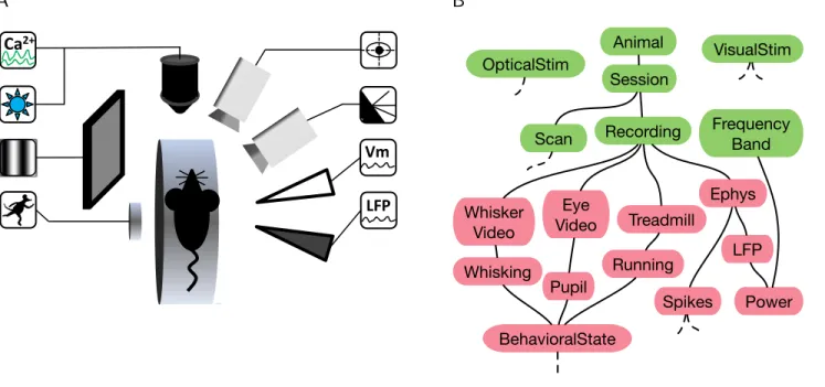
and calcium fluorescence signals), stimuli (visual display and optogenetic stimulation of targeted neuronal populations), and behaviors (locomotion, whisking, eye movements) [7]. Figure 1 A illustrates such an experiment.
To work with data from such studies, DataJoint users cre-ate a schema (or several schemas) comprising a collection of base relations to represent the various elements of the experiments (Fig. 1 B). Relations are DataJoint’s basic data representation and can be thought of as simple tables with a heading and a body. The heading specifies attribute names and datatypes. The body comprises a set of tuples of at-tribute values. Base relations are stored in the database whereasderived relations may be constructed from base re-lations for data queries. For detailed definitions of the Re-lational Data Model, see Table 1.
A base relation is created in the form of a class in MAT-LAB or Python (Fig. 1 C) that defines the relation’s head-ing. The heading definition comprises a description of the relation, dependencies on other base relations, and a set of attributes. Each attribute has a name, an optional default value, a datatype, and an optional description. Attributes that comprise theprimary key of the relation are separated from the remaining attributes by the divider---.
DataJoint provides all the functionality for accessing and manipulating data through the base relation classes.
Defining dependencies
The database must respect dependencies between data el-ements and prevent incomplete, orphaned, or mismatched data. DataJoint facilitates setting, enforcing, and display-ing data dependencies. The edges of the graph in the entity relationship diagram (ERD) in Fig. 1 B denote dependen-cies directed downward: relations below are dependent on relations above when connected. Chains of dependencies effectively set the order in which data must be populated. Thus the ERD serves as an effective communication tool for the overall data organization and the sequence of steps to be followed for data entry and processing. Each base relation can depend on multiple other relations but the dependency graph must be acyclic: a relation cannot depend on itself
or on other relations that depend on it directly or through other relations.
To create a dependency, the dependent relation’s data defini-tion must include the line-> Reference, whereReference is the class name of the referenced base relation.
Setting a dependency has two effects:
(a) the primary key attributes of the referenced relation are copied into the definition
(b) a foreign key constraint is created to the referenced re-lation.
The foreign key constraint causes the database to reject any new tuple in the dependent relation unless there exists a matching tuple in the referenced relation. Conversely, delet-ing a tuple from the referenced relation will cause all match-ing tuples in all the dependent relations to be deleted too. For example, when Sessiondepends onAnimal(Fig. 1 B), Animal’s primary key attributeanimalis automatically in-cluded inSession’s heading (Fig. 1 C and D). A new session cannot be entered for an animal that has not yet been en-tered; and when an animal is deleted, all its sessions will be deleted as well, along with all the dependent data below in the hierarchy.
Importantly for data dependencies, DataJoint treats tuples in relations as indivisible; dependencies are established be-tween whole tuples rather than bebe-tween attribute values. DataJoint methods modify relations only by inserting or deleting entire tuples and cannot update individual attribute values independently.
Such discipline guarantees that any changes of attribute val-ues will trigger recomputation of all dependent data. Of course, users can deliberately intervene and modify val-ues manually to bypass dependencies when necessary, pro-vided that they have been granted update privileges by the database administrator.
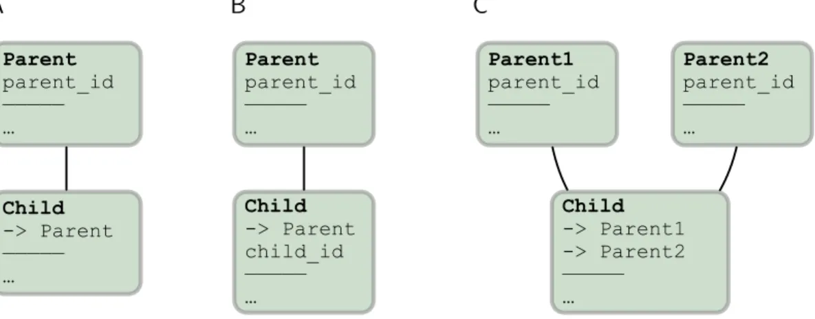
The primary keys and dependencies between base relations allow defining a rich variety of relationships between data elements. Three common types of relationships illustrate this point (Figure 2).
• In a one-to-one relationship (Fig. 2 A), relation Child declares a dependency within its primary key onParent but does not add any new attributes to its primary key. Thus the primary key for Child is the same as forParent: only one tuple inChildcan exists for each tuple inParent.
• In a one-to-many relationship (Fig. 2 B), relationChild declares a dependency within its primary on Parent but also declares an additional attribute child_id in its primary key, which allows Child to have multiple tuples matching each tuple inParent.
A
B
example.LFP (imported) # Local Field Potential (LFP) recorded from one electrode
-> example.Recording # dependent on Recording
channel : int # acquisition channel number ---
sampling_rate : int # (Hz) acquisition system sampling rate for this channel
voltage : longblob # (µV) raw local field potential recorded on this channel
lfp_time : longblob # (s) acquisition times
lfp_ts = CURRENT_TIMESTAMP : timestamp # automatic timestamp for each data entry in table
Vm LFP
Ca
2+ Animal Session Recording Whisker Whisking Eye Treadmill Running Spikes LFP BehaviorState*animal_id *session *recording *channel sampling_rate voltage lfp_time lfp_ts
100 1 1 1 30000 (BLOB) (BLOB) 2015-05-01 14:13:10 101 1 1 1 20000 (BLOB) (BLOB) 2015-01-19 13:43:39 101 2 1 2 20000 (BLOB) (BLOB) 2015-01-19 13:43:39 101 2 2 1 10000 (BLOB) (BLOB) 2015-01-27 18:54:01
A
B
C
D
Scan…
FrequencyBand Power VisualStim…
OpticalStim…
Pupil Example Schema Animal Session Recording Scan VisualStim OpticalStim LFP Frequency Band Eye Video Treadmill Spikes Whisker Video Power Pupil Running Whisking BehavioralState EphysC
1 @schema2 class Session(dj.Manual):
3 definition = """ # an experiment recording session for the given animal
4 -> Animal
5 session :smallint # recording session number for this animal
6
---7 user :varchar(16) # experimenter’s name
8 session_date :date # the date on which the recording session began
9 session_folder="" :varchar(200) # file path to the recorded data
10 notes="" :varchar(2000) # free-hand session notes
11 timestamp=CURRENT_TIMESTAMP :timestamp # automatic timestamp
12 """
D
animal session user session date session folder notes timestamp
1001 1 Jake 2015-10-29 /jake/20151029/1 success 2015-10-29 08:09:13
1001 2 Jake 2015-10-29 /jake/20151029/2 2015-10-29 14:35:48
1003 1 Shan 2015-10-30 /shan/20151030/1 2015-10-30 08:58:02
1003 2 Cathryn 2015-10-31 /cathryn/20151031 2015-10-31 15:04:13
Figure 1: An example experiment and its DataJoint schema. A. A neuroscience experiment with multiple stimulation and acquisition modalities (counterclockwise from top left corner): fluorescence imaging of calcium signals (Ca2+), light stimulation of optogenetic probes, visual stimulus, treadmill motion recording, local-field potential recording
(LFP), whole-cell patch membrane potential recording (Vm), video of whisker movements, video of eye movements. B.
The entity relationship diagram (ERD) of a DataJoint schema comprising base relations storing externally entered data (green) and automatically populated data (red). C.The Python class for the base relationSessionspecifying the relation’s heading. A dependency onAnimalis indicated with the arrow->. An additional primary key attribute,session, enables multiple sessions per animal. Dependent attributes are separated from primary key attributes by---. Each attribute has a name, an optional default value, a datatype, and an optional comment. D.Example contents ofSession. The vertical divider separates the primary key attributes ‘animal’ and ‘session‘ from the dependent attributes.
Relational Data Model
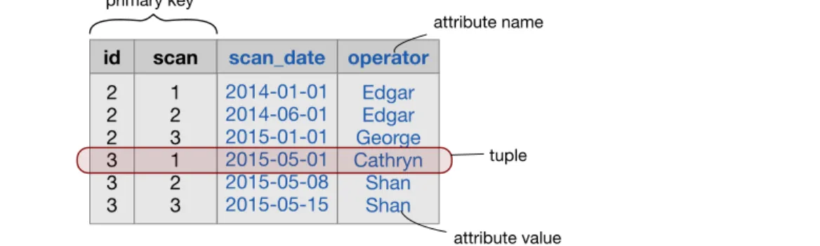
Relation All data are represented asrelations. A relation can be visualized as a table or a shreadsheet. It consists of aheading with attribute names and datatypes and abody comprising a set oftuples with values for each attribute.
2014-01-01 2014-06-01 2015-01-01 2015-05-01 2015-05-08 2015-05-15 2 2 2 3 3 3 id 1 2 3 1 2 3
scan scan_date operator
Edgar Edgar George Cathryn Shan Shan primary key attribute name tuple attribute value
We distinguish betweenbase relations andderived relations. A base relation has a dedicated class in MATLAB or Python and represents data stored directly in the database. Derived relations are formed from other relations by using relational operators (See Table 2). To create a new base relation, users create a new MATLAB or Python class subclassing from the DataJoint Relation class and define the relation’s heading. After that, users interact with the data by invoking these relation classes.
Schema A schema is a named collection of related base relations. A single project may store data across multiple schemas. Conversely, many schemas can be used for data shared by multiple projects.
Query Queries retrieve the data represented by a relation into the MATLAB or Python workspace.
Primary key Every relation has a primary key: a subset of its of attributes that uniquely identify each of its tuples. Two tuples with the same values of the primary key attributes cannot coexist in the same relation. The remaining attributes in the relation are called dependent attributes. When one relation includes some attributes that also belong to the primary key of another relation, they determine how tuples are grouped and related between the two relations.
Dependencies Base relations may form dependencies by referencing one another. Every tuple in a dependent rela-tion must have a matching tuple in the relarela-tions references by the dependency. Dependencies may cross schema boundaries.
ERD The entity relationship diagram or ERD is a graphical representation of base relations and their dependencies. Fig. 1 B depicts the ERD for a particular neuroscience experiment.
A
B
C
Parent parent_id ————— … Child -> Parent ————— … Parent parent_id ————— … Child -> Parent child_id ————— … Parent1 parent_id ————— … Child -> Parent1 -> Parent2 ————— … Parent2 parent_id ————— …Figure 2: Three common replationships defined through the dependencies and primary keys of base relations. A.A one-to-one relationship. B.A one-to-many (hierarchical) relationship. C.A combinatorial relationship.
• In a combinatorial relationship (Fig. 2 C), relation Child declares a dependency within its primary key on multiple relations. In this example, Child’s pri-mary key combines the pripri-mary key attributes from both Parent1 and Parent2. This means that Child holds tuples corresponding to any combination of tu-ples inParent1andParent2.
Examples of other types of relationships may be found in the online resources.
Querying data
DataJoint provides a minimal yet powerful set of operators on relations: restriction, projection, and join. These opera-tors allow transforming relations into new derived relations. Table 2 summarizes these operators.
The output of each relational operator is a proper relation in its own right with its primary key, uniquely named at-tributes, and the full range of data query methods. This property, calledalgebraic closure, allows expressings highly specific queries from existing queries intuitively and laconi-cally.
The starting point of any relational expression are base rela-tions represented by their classes. For example, after execut-ing the followexecut-ing assignment in either Python or MATLAB, rel = Ephys()
the variablerelwill represent the contents of the base rela-tionEphys, which represents electrophysiological recordings: local field potentials and spikes in our schema (Fig. 1 B). Restriction (represented by the logical AND operator&) se-lects a subset of tuples based on some condition. For ex-ample, Animal may be restricted by a structure specifying values of attributesspeciesandsex, in MATLAB,
r.species = ’mouse’ r.sex = ’M’
or in Python
r = dict(species=’mouse’, sex=’M’)
to produce the relation containing all male mice, male_mice = Animal() & r
Relations can be restricted by conditions in the form of char-acter strings, structures or structure arrays, or other rela-tions. For example, other relations may be restricted with male_miceeven in combination with other restrictions: rel = Ephys() & male_mice & ’sampling_rate > 10000’ The resultrelwill represent all Ephys recordings from male mice with acquisition sampling rates above 10 kHz when sampling_rateis an attribute ofEphys.
As another example, the relationRunningcontains episodes of the animals’ locomotion inferred from treadmill sensor recordings in relationTreadmill. Then the restriction rel = Session() & Running()
represents all sessions with at least one episode of running. Restrictions can also take the negative form using the- (mi-nus) operator. For example,
rel = (LFP() & Treadmill()) - Running()
contains all LFP recordings in sessions that included tread-mill recordings but no running episodes where found. The join operator (*) produces a relation comprising all pos-sible combinations of matching tuples from its two argument relations.
For example, the relation rel = Spikes() * LFP()
Relational algebra
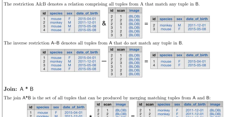
Relational operators operate on existing relations to producederived relations for answering a wide variety of specific queries. These operators do not retrieve any data from the database until the resulting expression is used tofetch the data. Relational operators are based on the concept ofmatching tuples: Two tuples are considered matchingunlessthey share an attribute with the same name but different values.
Restriction:
A & B
,
A – B
The restriction A&B denotes a relation comprising all tuples from A that match any tuple inB. (BLOB) (BLOB) (BLOB) (BLOB) (BLOB) (BLOB) 1 2 3 4 id species mouse monkey mouse mouse sex F M M F 2 2 2 3 3 3 id 1 2 3 1 2 3 scan image
&
=
2 3 id species monkey mouse sex M F date_of_birth 2015-04-01 2011-12-01 2015-05-08 2015-05-08 date_of_birth 2011-12-01 2015-05-08The inverse restrictionA–Bdenotes all tuples fromAthat do not match any tuple inB.
—
=
1 4 id species mouse mouse sex F F date_of_birth 2015-04-01 2015-05-08 1 2 3 4 id species mouse monkey mouse mouse sex F M M F date_of_birth 2015-04-01 2011-12-01 2015-05-08 2015-05-08 (BLOB) (BLOB) (BLOB) (BLOB) (BLOB) (BLOB) 2 2 2 3 3 3 id 1 2 3 1 2 3 scan imageJoin:
A * B
The joinA*Bis the set of all tuples that can be produced by merging matching tuples fromAandB:
*
=
(BLOB) (BLOB) (BLOB) (BLOB) (BLOB) (BLOB) 2 2 2 3 3 3 id 1 2 3 1 2 3scan species image
monkey monkey monkey mouse mouse mouse sex F F F M M M date_of_birth 2011-12-01 2011-12-01 2011-12-01 2015-05-08 2015-05-08 2015-05-08 1 2 3 4 id species mouse monkey mouse mouse sex F M M F date_of_birth 2015-04-01 2011-12-01 2015-05-08 2015-05-08 (BLOB) (BLOB) (BLOB) (BLOB) (BLOB) (BLOB) 2 2 2 3 3 3 id 1 2 3 1 2 3 scan image
All attributes inAandBthat share the same names must belong to the primary key in either relation.
Projection:
A.pro(attributes)
The projection A.pro(attributes) modifies the heading of A by selecting a subset of its attributes (project), renaming attributes (rename), computing new attributes (expand), and computing summary statistics from other relations (ag-gregate). The primary key attributes cannot be excluded from the resulting relation but may be renamed.
.pro(‘id -> animal_id’,‘image’) =
(BLOB) (BLOB) (BLOB) (BLOB) (BLOB) (BLOB) 2 2 2 3 3 3 id 1 2 3 1 2 3 scan image (BLOB) (BLOB) (BLOB) (BLOB) (BLOB) (BLOB) 2 2 2 3 3 3 animal_id 1 2 3 1 2 3 scan image date_of_birth 2011-12-01 2011-12-01 2011-12-01 2015-05-08 2015-05-08 2015-05-08
Please refer to the online documentation for more detailed descriptions.
will contain both spiking and LFP data for the sameEphys recordings.
Relational operators can be combined to produce highly spe-cific expressions. For example,
rel = Spikes() * LFP() & (Animal() * Session() &
’datediff(session_date, date_of_birth)<=28’) is similar to the previous example but the result is restricted to cases when the animals were 28 days old or younger at the start of the recording session. Since DataJoint passes its restriction conditions to SQL, restrictions can call SQL functions such as datediff here for computing the differ-ence between the dates. Note that session_date comes fromSessionwhereasdate_of_birthcomes fromAnimal. Thus the relationAnimal*Sessionhas both dates required for calculating the age.
The projection operator allows selecting and renaming at-tributes as well as computing new atat-tributes, including sum-mary statistics on other relations. Please refer to the online documentation for additional details.
Relation objects are only symbolic representations of the data and relational expressions are only symbolic manipu-lations. Once the desired relation is formulated, the actual data are retrieved from the database into a structure array using thefetchmethod
data = rel.fetch()
Entering and computing data
DataJoint distinguishes between manual and automated base relations. In the entity relationship diagram (Fig. 1 B), manual base relations are displayed as green nodes whereas automated base relations are displayed in red.
Manual base relations contain data entered by the exper-imenter or by acquisition software. They store data that are derived from external sources and are typically at the head of the dependency hierarchy. Users commonly edit manual relations directly in the form of a spreadsheet using third-party interfaces such as MySQL Workbench, Navicat, SequelPro, HeidiSQL, and others.
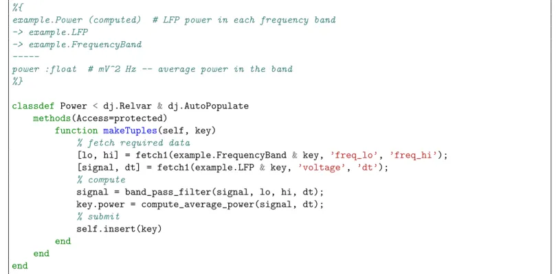
Automated base relations are filled automatically from MATLAB or Python with the help of their populate method. For example, Figures 3 and 4 list the complete implementation of thePowerbase relation, which computes the average power of the LFP signal for various frequency bands in our schema (Fig. 1 B).
Execution of the following commands will fill Powerfor all available data.
rel = Power() rel.populate()
The populate method always “knows” what needs to be computed using the base relation’s dependencies. It com-pares the contents of the base relation to those of its imme-diate neighbors upstream in the dependency hierarchy. The job list is defined as the join of the immediate upstream neighbors of the populated relation minus the population itself.
For example, Power depends on LFP and FrequencyBand. Then the restricted join
missing = LFP() * FrequencyBand() - Power() will express all combinations of tuples in LFP and FrequencyBand for whichPower does not yet have any en-tries. Each tuple in missingspecifies an isolated job to be performed for Power. This logic is implemented internally and is provided here only to help users understand what happens under the hood of apopulatecall.
When rel.populate() is called, it exe-cutes rel.makeTuples(key) (in MATLAB) or rel._make_tuples(key) (in Python) for the primary key value of each tuple inmissing.
Users specify the computation of new tuples for each item in missingusing themake-tuples callback method (Figures 3 or 4), which consists of three parts:
1. fetch the required data from other relations upstream in the dependency hierarchy, always restricting by the argumentkey,
2. use fetched data to compute attributes of the relation that are missing inkey,
3. create new tuples that combine the newly computed attributes and key and submit them to the database using theinsertmethod.
Eachmake-tuples call runs inside an isolatedtransaction so that its results do not become visible to other processes un-til the entire call completes successfully. If an error occurs during a make-tuples call, any partially populated data are discarded and never become visible to downstream compu-tations.
Thepopulatemethod has several options to control its be-havior. In particular, it has the option of using the built-in job reservation process to enable efficient distributed exe-cution. With job reservation enabled, users simply execute populateon multiple computers to run themake-tuplesjobs in parallel without conflicts. Please refer to the online doc-umentation forpopulateoptions and various techniques for customizing the processing chains.
Sharing data and distributed computation
Through the features described above, DataJoint naturally supports collaboration and distributed access by1 %{
2 example.Power (computed) # LFP power in each frequency band 3 -> example.LFP
4 -> example.FrequencyBand 5
---6 power :float # mV^2 Hz -- average power in the band
7 %}
8
9 classdef Power < dj.Relvar & dj.AutoPopulate
10 methods(Access=protected)
11 function makeTuples(self, key)
12 % fetch required data
13 [lo, hi] = fetch1(example.FrequencyBand & key, ’freq_lo’, ’freq_hi’); 14 [signal, dt] = fetch1(example.LFP & key, ’voltage’, ’dt’);
15 % compute
16 signal = band_pass_filter(signal, lo, hi, dt); 17 key.power = compute_average_power(signal, dt); 18 % submit 19 self.insert(key) 20 end 21 end 22 end
Figure 3: The class for the base relationPowerin MATLAB.
1 @schema
2 class Power(dj.Computed):
3 definition = """ # LFP power in each frequency band
4 -> LFP
5 -> FrequencyBand
6
---7 power :float # mV^2 Hz -- averge power in the band
8 """ 9
10 def _make_tuples(self, key): 11 # fetch required data
12 lo, hi = (FrequencyBand() & key).fetch1[’freq_lo’, ’freq_hi’] 13 signal, dt = (LFP() & key).fetch1[’voltage’, ’dt’]
14 # compute
15 signal = band_pass_filter(signal, lo, hi, dt) 16 power = compute_average_power(signal, dt) 17 # submit
18 self.insert1(dict(key, power=power))
• setting, enforcing, and communicating dependencies between data elements,
• keeping data definition and computation code together in the same class for easy review and sharing,
• storing and organizing data in a popular database man-agement system (MySQL) that can be accessed through a variety of third-party interfaces,
• allowing safe simultaneous access to the same data through standard transaction processing provided by MySQL, and
• providing an automatic and transparent job reservation process for conflict-free distributed processing.
Discussion
The relational data model has served as the theoretical foun-dation for the majority of mainstream database systems for over forty years and has been shown to be the most cogent and principled approach for representing and manipulating data of arbitrary complexity [10]. Yet, relational organiza-tion of data in science labs is still uncommon. This discon-nect is partly due to SQL’s position as the only wide-spread implementation of the relational model. SQL and its di-alects have deviated substantially from the simplicity of the relational data model and have overgrown with extraneous complexity.
Object-relational mappers (ORM) are software tools that map objects in computer memory to persistent storage such as relational databases. Since DataJoint constructs objects with persistently stored data, it can be classified as an ORM. Several other object-relational mappers are available for Python: SQLAlchemy, Django ORM, Peewee, PonyORM, SQLObject. They take a similar approach of converting ob-jects and idioms of the host programming language into SQL queries for processing by the database server. We are not aware of any ORM tools for MATLAB besides DataJoint. DataJoint addresses other needs than ORMs: it is specif-ically designed for providing a robust and intuitive data model for scientific data processing chains. As such, it does not attempt to simply mirror the features and capabilities of SQL. Instead, DataJoint imposes constraints and con-ventions to achieve the expressive power and simplicity of queries by strict adherence to the relational data model. In science, both the structure of the data and the queries evolve frequently. A simple, sound data model is of greater importance than in other database applications.
Some of the distinct constraints imposed by DataJoint in-clude the following:
1. All data are represented as proper relations with a pri-mary key and uniquely named attributes. This applies
to base and derived relations. Relational operators fol-low consistent rules for determining the primary key of its result. As a result, DataJoint’s operators are alge-braically closed, allowing building complex expressions from simpler expressions.
2. Data in base relations are updated only by inserting or deleting entire tuples: updates of attribute values are not supported. As discussed in the text, this limita-tion is necessary because referential constraints (foreign keys) enforce data dependencies only between tuples and not between individual attribute values.
3. Dependencies between base relations are acyclic, i.e. they cannot form loops. This restriction simplifies data definition but, perhaps counter-intuitively, does not prevent specifying arbitrary relationships between data elements, including directed graphs with cyclic de-pendencies, for example.
4. DataJoint limits relational operators to enforce clarity. For example, the projection operator (see Table 2 and online documentation) does not allow projecting out the primary key attributes. Consequently, the resulting re-lation has the same number of tuples as the original relation and every tuple is unique. If the user does in-tend to derive a relation with a different primary key, she must explicitly declare a base relation with this pri-mary key and use it to formulate the proper query. In practice, this is not a real limitation but a specific pre-scription of how data must be defined and manipulated in a uniform and explicit manner.
5. Foreign keys always link identically named attributes in both relations. This convention simplifies the specifica-tion of dependencies and of relaspecifica-tional operators. For ex-ample, a single join operator in DataJoint can perform the same work as the multiple forms and parameteri-zations of the JOIN operators in SQL. This convention is particularly important in DataJoint because it allows direct logical linking of relations separated by many in-termediate dependencies. In a large schema, this con-vention may lead to long composite primary keys low in the dependency hierarchy, but these are efficiently handled by MySQL’s storage engines.
DataJoint’s restricted relational data model represents a conceptual shift in database interactions: In SQL queries, users explicitly enumerate and match individual attributes. In contrast, DataJoint users formulate dependencies and queries at the level of entire relations. As a result, Data-Joint’s fast, intuitive, and expressive data definition and manipulation languages enable scientists to flexibly adapt their data processing chains to evolving demands.
Examples and resources
To benefit from DataJoint, users need not appreciate the various technical considerations underlying its capabilities. We encourage interested readers to review the online doc-umentation to get up and running with DataJoint quickly. For tutorials, a gallery of working schemas for MATLAB and Python, documentation, and references to scientific papers using DataJoint, please visit http://datajoint.github. com.
References
[1] D. Howe, M. Costanzo, P. Fey, T. Gojobori, L. Hannick, W. Hide, D. P. Hill, R. Kania, M. Schaeffer, S. St Pierre, S. Twigger, O. White, and S. Yon Rhee, “Big data: The future of biocuration,” Nature, vol. 455, pp. 47– 50, Sept. 2008.
[2] I. Maze, L. Shen, B. Zhang, B. A. Garcia, N. Shao, A. Mitchell, H. Sun, S. Akbarian, C. D. Allis, and E. J. Nestler, “Analytical tools and current challenges in the modern era of neuroepigenomics,” Nature Neu-roscience, vol. 17, pp. 1476–1490, Nov. 2014.
[3] Editorial, “Focus on big data,” Nature Neuroscience, vol. 17, pp. 1429–1429, Nov. 2014.
[4] N. R. Anderson, E. S. Lee, J. S. Brockenbrough, M. E. Minie, S. Fuller, J. Brinkley, and P. Tarczy-Hornoch, “Issues in Biomedical Research Data Management and Analysis: Needs and Barriers,” Journal of the Ameri-can Medical Informatics Association, vol. 14, pp. 478– 488, July 2007.
[5] E. R. Kandel, H. Markram, P. M. Matthews, R. Yuste, and C. Koch, “Neuroscience thinks big (and collabora-tively),”Nature Reviews Neuroscience, vol. 14, pp. 659– 664, Sept. 2013.
[6] J. Gray, D. T. Liu, M. A. Nieto-Santisteban, A. S. Sza-lay, G. Heber, and D. DeWitt, “Scientific Data Manage-ment in the Coming Decade,” ACM SIGMOD Record, vol. 34, pp. 35–41, Jan. 2005. also as MSR-TR-2005-10. [7] J. Reimer, E. Froudarakis, C. Cadwell, D. Yatsenko, G. Denfield, and A. Tolias, “Pupil Fluctuations Track Fast Switching of Cortical States during Quiet Wake-fulness,” Neuron, vol. 84, pp. 355–362, Oct. 2014. [8] E. Froudarakis, P. Berens, A. S. Ecker, R. J.
Cot-ton, F. H. Sinz, D. Yatsenko, P. Saggau, M. Bethge, and A. S. Tolias, “Population code in mouse V1 fa-cilitates readout of natural scenes through increased sparseness,”Nature Neuroscience, vol. 17, pp. 851–857, June 2014.
[9] E. F. Codd, “A Relational Model of Data for Large Shared Data Banks,”Commun. ACM, vol. 13, pp. 377– 387, June 1970.
[10] C. Date, SQL and relational theory: how to write ac-curate SQL code. O’Reilly Media, Inc., 2011.
[11] G. Manyam, M. A. Payton, J. A. Roth, L. V. Abruzzo, and K. R. Coombes, “Relax with CouchDB Into the non-relational DBMS era of bioinformatics,”Genomics, vol. 100, pp. 1–7, July 2012.
[12] C. Gnay, J. R. Edgerton, S. Li, T. Sangrey, A. A. Prinz, and D. Jaeger, “Database Analysis of Simulated and Recorded Electrophysiological Datasets with PANDO-RAs Toolbox,” Neuroinformatics, vol. 7, pp. 93–111, June 2009.
[13] E. D. Schutter, G. A. Ascoli, and D. N. Kennedy, “Re-view of Papers Describing Neuroinformatics Software,” Neuroinformatics, vol. 7, pp. 211–212, Dec. 2009. [14] S. L. Small, M. Wilde, S. Kenny, M. Andric, and
U. Hasson, “Database-managed Grid-enabled analysis of neuroimaging data: The CNARI framework,” Inter-national Journal of Psychophysiology, vol. 73, pp. 62– 72, July 2009.
[15] P. G. Brown, “Overview of sciDB: Large Scale Array Storage, Processing and Analysis,” in Proceedings of the 2010 ACM SIGMOD International Conference on Management of Data, SIGMOD ’10, (New York, NY, USA), pp. 963–968, ACM, 2010.
[16] B. Shi, J. Bourne, and K. M. Harris, “SynapticDB, Ef-fective Web-based Management and Sharing of Data from Serial Section Electron Microscopy,” Neuroinfor-matics, vol. 9, pp. 39–57, Mar. 2011.
[17] S. Pittendrigh and G. Jacobs, “Neurosys,” Neuroinfor-matics, vol. 1, pp. 167–176, June 2003.