Implementation Issues
Salvatore Orlando, Renzo Orsini, Alessandra Raffaetà, Alessandro Roncato Dipartimento di Informatica - Università Ca’ Foscari Venezia
{orlando, orsini, raffaeta, roncato}@dsi.unive.it Claudio Silvestri
Dipartimento di Informatica e Comunicazione - Università di Milano [email protected]
In this paper we investigate some issues and solutions related to the design of a Data Warehouse (DW), storing several aggregate measures about trajectories of moving objects. First we discuss the loading phase of our DW which has to deal with overwhelming streams of trajectory obser-vations, possibly produced at different rates, and arriving in an unpredictable and unbounded way. Then, we focus on the measure presence, the most complex measure stored in our DW. Such a measure returns the number of distinct trajectories that lie in a spatial region during a given temporal interval. We devise a novel way to compute an approximate, but very accurate, presence aggregate function, which algebraically combines a bounded amount of measures stored in the base cells of the data cube.
We conducted many experiments to show the effectiveness of our method to compute such an aggregate function. In addition, the feasibility of our innovative trajectory DW was validated with an implementation based on Oracle. We investigated the most challenging issues in realizing our trajectory DW using standard DW technologies: namely, the preprocessing and loading phase, and the aggregation functions to support OLAP operations.
Categories and Subject Descriptors: E.2 [DATA STORAGE REPRESENTATIONS]: General Terms: Design
Additional Key Words and Phrases: Data Warehouse, Aggregate Function
1. INTRODUCTION
Modern location-aware devices and applications deliver huge quantities of spatio-temporal data concerning moving objects, which must be either quickly processed for real-time applications, like traffic control management, or carefully mined for complex, knowledge discovering tasks. Even if such data usually originate as timed,
Copyright©2007 by The Korean Institute of Information Scientists and Engineers (KIISE). Per-mission to make digital or hard copies of part or all of this work for personal or classroom use is granted without fee provided that copies are not made or distributed for profit or commercial advantage and that copies bear this notice and the full citation on the first page. Copyrights for components of this work owned by others than KIISE must be honored. Abstracting with credit is permitted. To copy otherwise, to republish, to post on servers, or to redistribute to lists, requires prior specific permission and/or a fee. Request permission to republish from: Publicity Office, KIISE. FAX +82-2-521-1352 or [email protected].
located observations of well identified objects, they must often be stored in aggre-gate form, without identification of the corresponding moving objects, either for privacy reasons, or simply for the sheer amount of data which should be kept on-line to perform analytical operations. Such an aggregation is usually a complex task, and prone to the introduction of errors which are amplified by subsequent aggregation operations.
For these reasons, we propose an approach to the problem which is based on classical Data Warehouse (DW) concepts, so that we can adopt a well established and studied data model, as well as the efficient tools and systems already developed for such a model. Our DW is aimed at defining, as basic elements of interest, not the observations of the moving objects, but rather theirtrajectories, so that we can study properties such as average speed, travelled distance, maximum acceleration, presence of distinct trajectories. We assume the granularity of the fact table given by a regular three-dimensional grid on the spatial and temporal dimensions, where the facts are the set of trajectories which intersect each cell of the grid, and the measures are properties related to that set.
One of the main issues to face is the efficient population of the Trajectory DW (TDW) from streams of trajectory observations, arriving in an unpredictable and unbounded way, with different rates. The challenge is to exploit a limited amount of buffer memory to store a few incoming past observations, in order to correctly reconstruct the various trajectories, and compute the needed measures for the base cells, reducing as much as possible the approximations.
The model of our TDW and the corresponding loading issues have been intro-duced in [Braz et al. 2007]. In this paper we discuss in detail the loading and computation of a complex aggregate measure, the presence, which can be defined as the number of distinct trajectories lying in a cell. Such a measure poses non triv-ial computational problems. On one hand, in the loading phase, only a bounded amount of memory can be used for analysing the input streams. This suffices for trajectory reconstruction, but in some cases we may still count an object, with mul-tiple observations in the same cell, more than once. Hence the measure presence computed for base cells is in general an approximation of the exact value. A second approximation is introduced in the roll-up phase. In fact, since the roll-up function for the measure presence is, asdistinct count, aholisticfunction, it cannot be com-puted using a finite number of auxiliary measures starting from sub-aggregates. Our proposal is based on an approximate, although very accurate, presence aggregate function, which algebraically combines a bounded amount of other sub-aggregate measures, stored in the base cells of the grid.
The paper will provide a thorough analysis of the above mentioned technique, focusing, in particular, on the errors introduced by the approximations. From our tests, our method turned out to yield an error which is sensibly smaller than the one of a recently proposed algorithm [Tao et al. 2004], based onsketches, which are a well known probabilistic counting method in database applications [Flajolet and Martin 1985].
We also realized a prototype of our TDW, in order to investigate its feasibility when using commodity warehousing tools, like the Oracle one. The first challenge is the ETL process of the DW: by exploiting a few memory, we have to transform Journal of Computing Science and Engineering, Vol. 1, No. 2, December 2007
a stream of trajectory observations on-the-fly and aggregate them to update the base cells of our spatio-temporal cube. Using a Java application, performing the data transformation, and a specific loading method available in the Oracle suite, we were able to elaborate and load about 7000 observations per second. The other challenge is the efficient computation of our approximate aggregate function, used to roll-up the presence measure.
The rest of the paper is organised as follows. In Section 2 we present some related work whereas in Section 3 we discuss the issues related to the representation of trajectories. In Section 4 we recall our TDW model and in Section 5 we describe the loading phase of the measure presence and the aggregate functions supporting the roll-up operation. Then in Section 6 the approximation errors of the loading and roll-up phases are studied, both analytically and with the help of suitable tests. Section 7 focuses on our experience in designing a prototype of our TDW using Oracle. Finally, Section 8 draws some conclusion.
2. RELATED WORK
Research on spatial multidimensional data models is relatively recent. The pioneer-ing work of Han et al. [Han et al. 1998] introduces a spatial data cube model which consists of both spatial and non-spatial dimensions and measures. Additionally, it analyses how OLAP operations can be performed in such a spatial data cube. Then, several authors have proposed data models for spatial data warehouses at a con-ceptual level (e.g., [Pedersen and Tryfona 2001; Damiani and Spaccapietra 2006]). Unfortunately, none of these approaches deal with objects moving continuously in time.
Research on moving objects has focused on modelling [Sistla et al. 1997; Güting et al. 2000] and on indexing such spatio-temporal data [Kollios et al. 1999; Pfoser et al. 2000], whereas the definition of TDWs is still an open problem. An issue that is gaining increasingly interest in the last years and that is relevant for the devel-opment of a TDW concerns the specification and efficient implementation of the operators for spatio-temporal aggregation. Nevertheless a standard set of operators (e.g, operators like Avg, Min, Max in SQL) has not yet been defined. A first com-prehensive classification and formalisation of spatio-temporal aggregate functions is presented in [Lopez et al. 2005]. The aggregate operations are defined as functions that, applied to a collection of tuples, return a single value. To generate the collec-tion of tuples to which these operacollec-tions are applied, the authors distinguish three kinds of methods: group composition, partition composition and sliding window composition. On the other hand, in [Papadias et al. 2002; Tao and Papadias 2005] techniques for the computation of aggregate queries are developed based on the combined use of specialised indexes and materialisation of aggregate measures. For instance [Papadias et al. 2002] introduces theaRB-tree, which consists of two types of indexes: a host index and some measure indexes. The host index is an R-tree which manages the region extents, and associates with these regions an aggregate information over all the timestamps of interest. Additionally, for each entry of the host index, a B-tree containing the time-varying aggregate data is defined.
As shown in [Tao et al. 2004], most of these indexes, like aRB-trees, can suffer from thedistinct counting problem, i.e., if an object remains in the query region for Journal of Computing Science and Engineering, Vol. 1, No. 2, December 2007
several timestamps during the query interval, it will be counted multiple times in the result. In fact such indexes store, for each region, an aggregate measure and they forget the identifiers of the objects.
To cope with this issue, [Tao et al. 2004] proposes an approach which com-bines spatio-temporal indexes with sketches, a traditional approximate counting technique based on probabilistic counting [Flajolet and Martin 1985]. The index structure is similar to aRB-trees but differs from them in the querying algorithms since one can exploit the pruning power of the sketches to define some heuristics which allow to reduce the query time.
It is worth noticing that the above cited works on aggregation methods do not take into account the fact that the spatio-temporal observations belong to moving objects. Instead they treat such observations as unrelated points. For a data ware-house of trajectories, we will show that it is important to exploit such relationships existing among observations. For example, in order to compute the approximate number of distinct trajectories intersecting a given spatio-temporal area, in this paper we exploit the knowledge about how many objects move from one region to the close ones, thus improving the result of roll-up operations.
3. TRAJECTORY REPRESENTATION
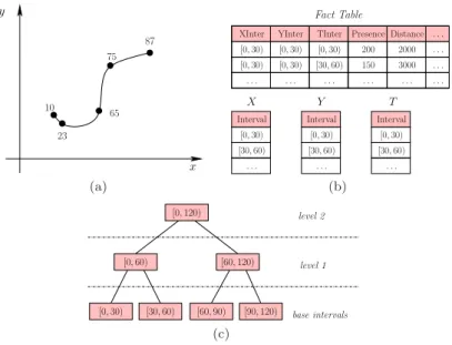
In real-world applications the movements of a spatio-temporal object, i.e. its tra-jectory, is often given by means of a finite set ofobservations. This is a finite subset of points, calledsampling, taken from the actual continuous trajectory. Figure 1(a) shows a trajectory of a moving object in a 2D space and a possible sampling, where each point is annotated with the corresponding time-stamp. It is reasonable to expect that observations are taken at irregular rates for each object, and that there is no temporal alignment between the observations of different objects.
Formally, letT Sbe a stream ofsamplings of 2D trajectoriesT S={Ti}i∈{1,...,n}.
EachTi is the sampling for an object trajectory: Ti= (IDi, Li), whereIDi is the identifier associated with the object and Li ={L1i, L2i, . . . , LMii } is a sequence of observations. Each observation Lji = (tij, xji, yij) represents the presence of an object at location(xji, yij)and time tji. The observations are temporally ordered, i.e.,tji < tji+1.
In many situations, e.g., when one is interested in computing the cumulative number of trajectories in a given area, an (approximate) reconstruction of each trajectory from its sampling is needed. Among the several possible solutions, we will focus onlocal interpolation. According to this method, although there is not a global function describing the whole trajectory, objects are assumed to move be-tween the observed points following some rule. For instance, alinear interpolation function models a straight movement with constant speed, while other polynomial interpolations can represent smooth changes of direction. The linear (local) inter-polation, in particular, seems to be a quite standard approach to the problem (see, for example, [Pfoser et al. 2000]), and yields a good trade-off between flexibility and simplicity. Hence in this paper we will adopt this kind of interpolation. However, it is straightforward to use a different interpolation, based, for example, on additional information concerning the environment traversed by the moving objects.
Starting from the stream of samplings, T S, we want to investigate if DW tech-Journal of Computing Science and Engineering, Vol. 1, No. 2, December 2007
x 10 75 65 23 y 87 (a) X Y T Fact Table . . . . . . . . . [0,30) . . . [0,30) . . . [0,30) [30,60) . . . . . . . . .
XInter YInter TInter Distance
200 2000 [0,30) [0,30) 150 3000 . . . Interval [0,30) [30,60) . . . Interval [0,30) [30,60) . . . Interval [0,30) [30,60) . . . Presence (b) [0,30) [0,60) [0,120) [60,120) [60,90) [30,60) [90,120) level 1 level 2 base intervals (c)
Figure 1. (a) A 2D trajectory with a sampling, (b) a DW example, and (c) a concept (set-grouping) hierarchy.
nologies [Chaudhuri and Dayal 1997; Han et al. 2005], and thus the concept of multidimensional and multilevel data model, can be used to store and compute specificmeasures regarding trajectories.
4. FACTS, DIMENSIONS, MEASURES AND AGGREGATE FUNCTIONS We define a DW model by means of a star schema, as simple and generic as pos-sible. The facts of our TDW are the set of trajectories which intersect each cell of the grid. Some typical properties we want to describe, i.e., the measures, are the number of trajectories, their average, maximum/minimum speed, the covered distance. The dimensions of analysis consist of the spatial dimensions X, Y rang-ing over spatial intervals, and the temporal dimension T ranging over temporal intervals. We assume a regular three-dimensional grid obtained by discretizing the corresponding values of the dimensions and then we associate with them a set-grouping hierarchy. A partial order can thus be defined among groups of values, as illustrated in Figure 1(c) for a temporal or a spatial dimension. Note that in the TDW of Figure 1(b), the basic information we represent concerns the set of trajec-tories intersecting the spatio-temporal cell having for eachX,Y, orT dimensions as minimum granularity 30 units, measured in the corresponding unit of measure. The hierarchy is not explicitly represented (we refer the reader to Figure 4 for a more complete picture).
It is interesting to investigate whether some pre-computation must be carried out on the trajectory observations in order to feed the TDW. Some measures re-quire little pre-computation, and can be updated in the TDW as soon as single observations of the various trajectories arrive, others need all the observations of a trajectory to be received, before updating the TDW. In [Braz et al. 2007] we Journal of Computing Science and Engineering, Vol. 1, No. 2, December 2007
classified the measures according to an increasing amount of pre-calculation effort. For instance, in order to compute the average, maximum/minimum speed and the covered distance by the trajectories intersecting a cell we need two consecutive ob-servations since we have to infer the trajectory route through interpolation. On the other hand, the measure number of observations falling in a cell can be updated directly using each single observation.
We can build the spatial data cube [Gray et al. 1997] as the lattice of cuboids, where the lowest one (base cuboid) references all the dimensions at the primitive abstraction level, while the others are obtained by summarising on different subsets of the dimensions, and at different abstraction levels along the concept hierarchy. In order to denote a component of the base cuboid we will use the termbase cell, while we will simply usecell for a component of a generic cuboid.
In order to summarise the information contained in the base cells, Gray et al. [Gray et al. 1997] categorise the aggregate functions into three classes based on the space complexity needed for computing a super-aggregate starting from a set of sub-aggregates already provided, e.g., the sub-aggregates associated with the base cells of the DW. The classes are the following:
(1) Distributive. The super-aggregates can be computed from the sub-aggregates.
(2) Algebraic. The super-aggregates can be computed from the sub-aggregates together with afinite set of auxiliary measures.
(3) Holistic. The super-aggregates cannot be computed from sub-aggregates, not even using any finite number of auxiliary measures.
For example, the super-aggregates for the distance and the maximum/minimum speed are simple to compute because the corresponding aggregate functions are distributive. In fact once the base cells have been loaded with the exact measure, for the distance we can accumulate such measures by using the functionsum whereas for maximum/minimum speed we can apply the function max/min. The super-aggregate for theaverage speed is algebraic: we need the pair of auxiliary measures hdistance,timei where distance is the distance covered by trajectories in the cell and time is the total time spent by trajectories in the cell. For a cell C arising as the union of adjacent cells, the cumulative function performs a component-wise addition, thus producing a pairhdistancef,timefi. Then the average speed inC is given bydistancef/timef.
5. THE MEASURE PRESENCE
In this paper we focus on the measurepresencewhich returns the number ofdistinct trajectories in a cell. As already remarked, a complication in dealing with such a measure is due to the distinct count problem and this has an impact on both the loading of the base cells and on the definition of aggregate functions able to support the roll-up operation.
5.1 Aggregate functions
According to the classification presented in Section 4, the aggregate function to compute the presence isholistic, i.e., it needs the base data to compute the result in all levels of dimensions. Such a kind of functions represents a big issue for DW Journal of Computing Science and Engineering, Vol. 1, No. 2, December 2007
technology, and, in particular, in our context, where the amount of data is huge and unbounded. A common solution consists in computing holistic functions in an approximate way.
We propose two alternative and non-holistic aggregate functions that approx-imate the exact value of the presence. These functions only need a small and constant memory size to maintain the information to be associated with each base cell of our TDW, from which we can start computing a super-aggregate.
The first aggregate function is distributive, i.e., the super-aggregate can be com-puted from the sub-aggregate, and it is called PresenceDistributive. We assume
that the only measure associated with each base cell is the exact (or approximate) count of all the distinct trajectories intersecting the cell. Therefore, the super-aggregate corresponding to a roll-up operation is simply obtained by summing up all the measures associated with the cells. This is a common approach (exploited, e.g., in [Papadias et al. 2002]) to aggregate spatio-temporal data. However, our experiments will show that this aggregate function may produce a very inexact ap-proximation of the effectivepresence, because the same trajectory might be counted multiple times. This is due to the fact that in the base cell we do not have enough information to perform adistinct count when rolling-up.
The second aggregate function is algebraic, i.e., the super-aggregate can be com-puted from the sub-aggregate together with afinite set of auxiliary measures, and it is calledPresenceAlgebraic. In this case each base cell stores a tuple of measures.
Besides the exact (or approximate) count of all thedistinct trajectories intersecting the cell, the tuple includes other measures which are used when we compute the super-aggregate. The additional measures are helpful to correct the errors, caused by the duplicates, introduced by the functionPresenceDistributive.
More formally, letCx,y,tbe a base cell of our cuboid, wherex,y, and t identify intervals of the form[l, u), in which the spatial and temporal dimensions are parti-tioned. The tuple associated with the cell consists ofCx,y,t.presence,Cx,y,t.crossX,
Cx,y,t.crossY, andCx,y,t.crossT.
—Cx,y,t.presence is the number ofdistinct trajectories intersecting the cell.
—Cx,y,t.crossX is the number of distinct trajectories crossing the spatial border betweenCx,y,t andCx+1,y,t.
—Cx,y,t.crossY is the number of distinct trajectories crossing the spatial border betweenCx,y,t andCx,y+1,t.
—Cx,y,t.crossT is the number of distinct trajectories crossing thetemporal border betweenCx,y,t andCx,y,t+1.
Let Cx0,y0,t0 be a cell consisting of the union of two adjacent cells with respect
to a given dimension, namelyCx0,y0,t0 =Cx,y,t∪Cx+1,y,t. In order to compute the
super-aggregate corresponding toCx0,y0,t0, we proceed as follows: PresenceAlgebraic(Cx,y,t∪Cx+1,y,t) =Cx0,y0,t0.presence=
=Cx,y,t.presence + Cx+1,y,t.presence − Cx,y,t.crossX
(1) The other measures associated withCx0,y0,t0 can be computed in this way:
Cx0,y0,t0.crossX =Cx+1,y,t.crossX (2)
Cx0,y0,t0.crossY =Cx,y,t.crossY +Cx+1,y,t.crossY (3) Journal of Computing Science and Engineering, Vol. 1, No. 2, December 2007
Cx,y+1,t Cx,y,t Cx+1,y,t Cx+1,y+1,t (a) Cx,y+1,t Cx+1,y+1,t Cx,y,t Cx+1,y,t (b)
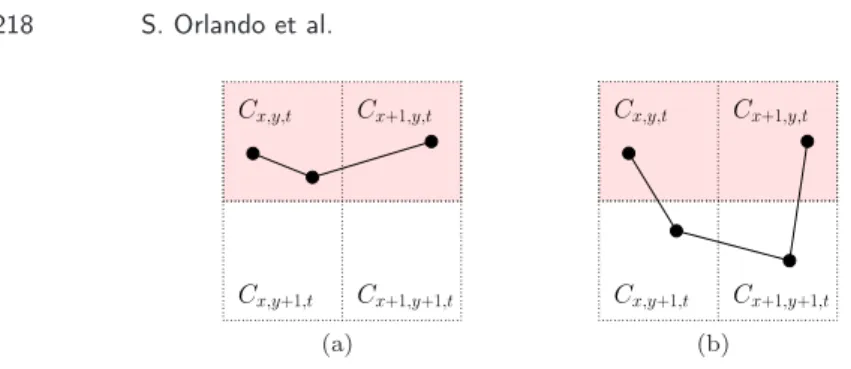
Figure 2. A trajectory (a) that is correctly counted, and (b) that entails duplicates during the roll-up.
Cx0,y0,t0.crossT=Cx,y,t.crossT+Cx+1,y,t.crossT (4) Equation (1) can be thought of as an application of the well known Inclusion/Exclusion principle: |A∪B|=|A|+|B| − |A∩B|for all setsA,B. Suppose that the elements included in the setsAandB are just the distinct trajectories intersecting the cells
Cx,y,t andCx+1,y,t, respectively. Hence, their cardinalities|A|and|B|exactly cor-respond toCx,y,t.presence and Cx+1,y,t.presence. Then Cx,y,t.crossX is intended to approximate|A∩B|, but, notice that, unfortunately, in some casesCx,y,t.crossX is not equal to |A∩B|, and this may introduce errors in the values returned by PresenceAlgebraic. Figure 2(a) shows a trajectory that will be correctly counted,
since it crosses the border between the two cells to be rolled-up. Conversely, Fig-ure 2(b) shows a very agile and fast trajectory, which will be counted twice during the roll-up, since it is not accounted in Cx,y,t.crossX, even if it should appear in |A∩B|. In fact, the trajectory intersects both Cx,y,t and Cx+1,y,t, but does not cross theX border between the two cells.
In order to understand Equations 2–4, notice that the rightX border of the new cellCx0,y0,t0 is the correspondingX border of the rightmost cellCx+1,y,t, hence the
number of distinct trajectories crossing theX border ofCx0,y0,t0 isCx+1,y,t.crossX
(Equation 2). Instead, the topY border ofCx0,y0,t0 is the union of the corresponding
borders of the component cellsCx,y,t and Cx+1,y,t. This is why in the Equation 3 we take the sum ofCx,y,t.crossY andCx+1,y,t.crossY. Similar considerations apply to Equation 4.
5.2 Loading phase
In this section we deal with the problem of feeding the DW, i.e., the base cells of our base cuboid, with suitable sub-aggregate measures, from which the aggregate functions compute the super-aggregates.
We recall that trajectory observations arrive in streams at different rates, in an unpredictable and unbounded way. In order to limit the amount ofbuffer memory needed, it is essential to store information only aboutactive, i.e., not ended trajecto-ries. In our simple model of trajectory sampling, since we do not have an end-mark associated with the last observation of a given trajectory, the system module that is responsible for feeding data decides to consider a trajectory asended when for a long time interval no further observation for the object has been received.
In the following we present two options to compute the sub-aggregates stored in each base cell Cx,y,t, namely Cx,y,t.presence, Cx,y,t.crossX, Cx,y,t.crossY, and Journal of Computing Science and Engineering, Vol. 1, No. 2, December 2007
Cx,y,t.crossT, which are used by the aggregate functions PresenceDistributive and
PresenceAlgebraic.
(1) Single observations. Considering a single observation at a time, without buffering any past observation, we can only update/increment the measure
Cx,y,t.presence. As a consequence, we cannot computePresenceAlgebraic, since Cx,y,t.crossX,Cx,y,t.crossY andCx,y,t.crossT are not available.
(2) Pairs of observations. We consider a pair of observations consisting of the currently received observationLji of trajectoryTi, with the previously buffered
Lji−1. Using this pair of points, we canlinearly interpolate the trajectory, thus registering further presences for the cells only traversed byTi.
Moreover, if we store in the buffer not only Lji−1, but also the last base cell
Cx,y,t that was modified on the basis of trajectoryTi, we can reduce the num-ber of duplicates by simply avoiding updating the measure whenLji falls into the sameCx,y,t. It is worth noting that since this method only exploits a very small buffer, it is not able to remove all the possible duplicates from the stored presence measures. Consider, for example, three observations of the same tra-jectory, all occurring within the same base time interval. If the first and the third points fall into the same cellCx,y,t, but the second one falls outside (e.g., intoCx,y+1,t), this method will store a duplicate count inCx,y,t.presence when the third observation is encountered.
Finally, by exploiting linear interpolation, we can also identify the cross points of each base cell, and accordingly update the various sub-aggregatesCx,y,t.crossX,
Cx,y,t.crossY, andCx,y,t.crossT.
5.3 Accuracy of the approximate aggregate function
Let us give an intuitive idea of the errors introduced by the aggregate function PresenceAlgebraic, starting from the measures loaded in the base cells by the method
Pairs of observations. Notice that the overall error can be obtained as the sum of the errors computed for each single trajectory in isolation.
Let us first consider the simplest case: a trajectory is a line segment l. In this case, no roll-up errors are introduced in the computation of presence. In fact, letCx0,y0,t0 be the union of two adjacent cells, Cx,y,t and Cx+1,y,t, i.e., Cx0,y0,t0 =
Cx,y,t S
Cx+1,y,t, andl intersectCx0,y0,t0. Then by definition:
PresenceAlgebraic(Cx,y,t S
Cx+1,y,t) =
Cx,y,t.presence+Cx+1,y,t.presence−Cx,y,t.crossX
Ifl intersects theX border, then correctly PresenceAlgebraic(Cx0,y0,t0) = 1 + 1−1.
Otherwise, Cx,y,t.crossX = 0, but l intersects only one of the two cells. Hence PresenceAlgebraic(Cx0,y0,t0) = 1 + 0−0 orPresenceAlgebraic(Cx0,y0,t0) = 0 + 1−0.
This result can be extended to a trajectory which is composed of a set of line segments whose slopes are in the same octant of the three-dimensional coordinate system. Let us calluni-octant sequencea maximal sequence of line segments whose slopes are in the same octant. Clearly, every trajectory can be uniquely decomposed in uni-octant sequences and, in the worst case, the error introduced by the aggregate functionPresenceAlgebraic will be the number of uni-octant sequences composing a
trajectory.
6. EVALUATING APPROXIMATE SPATIO-TEMPORAL AGGREGATES In this section we evaluate our method to approximate the measure presence and we are also interested in comparing it with a distributive approximation recently proposed [Tao et al. 2004]. The method is based onsketches, a traditional technique based on probabilistic counting, and in particular on the FM algorithm devised by Flajolet and Martin [Flajolet and Martin 1985].
6.1 FM sketches
FM is a simple, bitmap-based algorithm to estimate the number of distinct items. In particular, each entry in the sketch is a bitmap of length r = logU B, where
U B is an upper bound on the number of distinct items. FM requires a hash functionhwhich takes as input an object IDi(in our case a trajectory identifier), and outputs a pseudo-random integer h(i)with a geometric distribution, that is,
P rob[h(i) =v] = 2−v for v ≥1. Indeed, his obtained by combining a uniformly distributed hash functionh0, and a functionρthat selects the least significant 1-bit
in the binary representation ofh0(i). The hash function is used to update ther-bit
sketch, initially set to 0. For every objecti(e.g., for every trajectory observation in our stream), FM thus sets theh(i)-thbit. In the most naive and simple formulation, after processing all objects, FM finds the position of the leftmost bit of the sketch that is still equal to 0. If kis this position, then it can be shown that the overall object countncan be approximated with 1.29×2k.
Unfortunately, this estimation may entail large errors in the count approxima-tion. The workaround proposed in [Flajolet and Martin 1985] is the adoption ofm
sketches, which are all updated by exploiting a different and independent hash func-tion. Letk1, k2, . . . , km be the positions of the leftmost 0-bit in themsketches. The new estimate ofnis1.29×2ka, wherek
a is the mean of the variouskivalues, i.e. ka = (1/m)
Pm
i=1ki. This method reduces the standard error of the
estima-tion, even if it increases the expected processing cost for object insertion. The final method that reduces the expected insertion cost back to O(1) is Probabilistic Counting with Stochastic Averaging (PCSA). The trick is to randomly select, for each object to insert, one of themsketches. Each sketch thus becomes responsible for approximatelyn/m(distinct) objects.
An important feature of FM sketches is that they can be merged in adistributive way. Suppose that each sketch is updated on the basis of a different set of objects. We can merge a pair of sketches together, in order to get a summary of the number of distinct items seen over the union of both sets of items, by simply taking the bitwise-ORof the corresponding bitmaps. We can find a simple application of these FM sketches in our TDW. First, we can exploit a small logarithmic space for each base cell, used to store a sketch that approximates the distinct count of trajectories seen in the corresponding spatio-temporal region. The distributive nature of the sketches can then be used to derive the counts at upper levels of granularities, by simply OR-ing the sketches at the lowest granularities.
6.2 Experimental Setup
Datasets. In our experiments we have used several different datasets. Most of them are synthetic ones, generated by the traffic simulator described in [Brinkhoff Journal of Computing Science and Engineering, Vol. 1, No. 2, December 2007
2002], but also some real-world sets of trajectories, presented in [Frentzos et al. 2005], were used.
Due to space limitations, we present only the results produced for one of the synthetic datasets and for one real dataset. The synthetic dataset was generated using a map of the San Joaquin road network (US Census code 06077), and contains the trajectories of 10000 distinct objects monitored for 50 time units, with an average trajectory length of 170k space units. The real-world dataset contains the trajectories of 145 school buses. The average number of sample points per trajectory is 455, and, differently from the case of synthetic data, not all points are equally distant in time. Since the setting does not suggest a specific granularity, we define as a standard base granularity for each dimension the average difference of coordinate values between two consecutive points in a trajectory. We will specify granularities as multiples of this base granularityg. For the synthetic datasetg= (1,2000,2000)
and for the school buses oneg= (2,100,100), where the granularities of the three dimensions are in the order: t,x,y.
Accuracy assessment. Vitter et al. [Vitter et al. 1998] proposed several error measures. We selected the one based on absolute error, which appears to be the most suited to represent the error on data that will be summed. Instead of the ∞−norm, however, we preferred to use the1−normas a normalisation term, since it is more restrictive and less sensible to outliers.
The formula we used to compute the normalised absolute error for all the OLAP queriesq in a setQis thus the following:
Error= ° ° ° fM−M ° ° ° 1 kMk1 = P q∈QP|Mfq−Mq| q∈QMq (5) whereMfq is the approximate measure computed for queryq, whileMq is its exact value. The various queries qmay either refer to base cells, or to cells at a coarser level of granularity. In particular, we used this error measure for evaluating the loading errors at the level of base cells, and theroll-up errorsat the level of coarser cells. In all these cases, we always applied Equation (5) to evaluate the errors entailed by a setQof queries at uniform granularity.
6.3 Experimental Evaluation
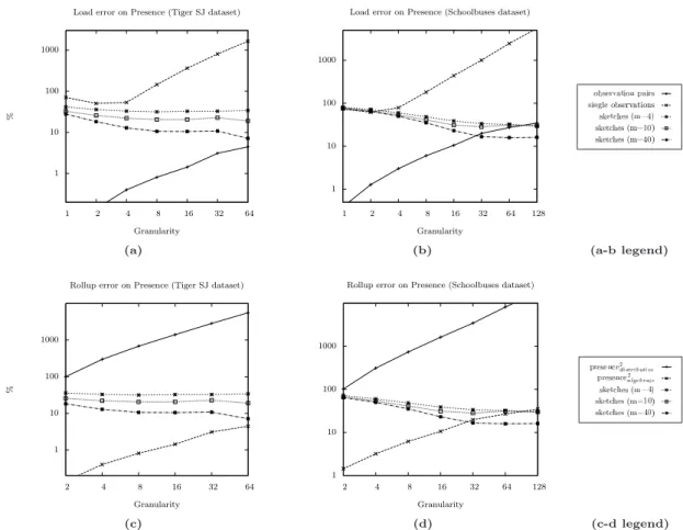
First we evaluate the errors in the loading phase of our TDW. During this phase, the reconstruction of the trajectories takes place. Figures 3.(a) and 3.(b) show the accuracy of the loaded (sub-aggregate) presence, for different granularities of the base cells. In particular, the two figures illustrate the normalised absolute error as a function of the size of base cells for the two datasets.
Let us focus on the curves labelledsingle observations. In this case we simply fed the TDW with each single incoming trajectory observation, without introducing any additional interpolated point. For small granularities, errors are mainly due to the fact that some cells are traversed by trajectories, but no observation falls into them. On the other hand, for very coarse granularities, the main source of errors is the duplicate observations of the same trajectory within the same cell. There exists an intermediate granularity (around2gfor these particular datasets) which Journal of Computing Science and Engineering, Vol. 1, No. 2, December 2007
represents the best trade-off between the two types of errors, thus producing a small error.
Then consider the curves labelled asobservation pairs. In this case the presence (sub-aggregate) measure of the base cells of the TDW is loaded by exploiting a buffer, which stores information about active trajectories. For each of these tra-jectories, the buffer only stores the last received observation. This information is used to reduce the errors with respect to the previous feeding method, by adding interpolated points, and also avoiding to record duplicates in the base cells. The resulting normalised absolute error is close to 0 for small granularities, and it re-mains considerably small for larger values. For very large granularities, a buffer that only stores information about the last previously encountered observation does not suffice to avoid recording duplicates in the base cells.
The other curves in Figure 3(a) and 3(b) represent the error introduced in the base cell by approximating the presence (sub-aggregate) measure by using sketches. It is worth noting that also to load the sketch-base cells, we added further interpolated observations, by using the buffer during the loading phase. Although the error slightly decreases when a larger number of sketches, m, is used for each cell, it remains considerably larger than the curve labelled asobservation pairs, except for coarse granularities and a large number of sketches (m= 40).
The second set of tests, whose results are reported in Figures 3(c) and 3(d), regards the errors introduced by rolling-up our cube, starting from the base cells at granularityg. The base granularityg= 1 used for these tests was the same as the one in Figures 3(a-b), while the method used to load the base cells wasobservation pairs. Therefore the normalised absolute error at the various base cells was close to
0. In all the roll-up tests, the error is averaged by submitting many queries at a given granularityg0 > g,g0 =n·g. Each query computes the presence measure associated
with a distinct coarse-grain cell, obtained by aggregating different adjacent base cells. As an example of query, eight adjacent base cells are aggregated to make one cell of granularity2·g.
As shown by the corresponding curves, thedistributive aggregate function (sum) quickly reaches very large errors as the roll-up granularity increases. This is due to the duplicated counting of the same trajectories, when they are already counted by multiple sub-aggregates. Conversely, we obtained very accurate results with our algebraic method, with an error always smaller than 10%, for most granularities (except for very coarse ones and 40 sketches). Finally, the distributive function (or) used to aggregate sketches produce much larger errors than our method, even because such large errors are already present in the sketches stored in the base cells. However, a nice property of sketches is that the cumulative errors do not increase, and, are actually often reduced when rolling-up, but sketches also exploit much more memory per cell. In case of m= 40, the memory usage of the sketch-based method is one order of magnitude larger than our algorithm. Thus it is remarkable that our method achieves a better accuracy in most cases, in spite of this unfavourable bias.
1 10 100 1000 1 2 4 8 16 32 64 % Granularity
Load error on Presence (Tiger SJ dataset)
1 10 100 1000 1 2 4 8 16 32 64 128 Granularity
Load error on Presence (Schoolbuses dataset)
(a) (b) (a-b legend)
1 10 100 1000 2 4 8 16 32 64 % Granularity
Rollup error on Presence (Tiger SJ dataset)
1 10 100 1000 2 4 8 16 32 64 128 Granularity
Rollup error on Presence (Schoolbuses dataset)
(c) (d) (c-d legend)
Figure 3. Errors on different datasets during the load and roll-up phases as a function of the granularity. Granularity is expressed as a multiple of the minimal granularitygfor load, and of the base granularitygfor roll-up (note logarithmic scale for both axes).
7. PROTOTYPE OF OUR TDW USING ORACLE
In this section we will focus on the implementation of our TDW. In particular we will discuss the most challenging issues with respect to a traditional DW: namely, the preprocessing phase to transform data to be loaded, and the aggregation functions, necessary to support OLAP operations. As described in Section 5.2, the set of streaming observations are not enough to correctly compute the measures, e.g., we have to generate new points through interpolations. Moreover, the common aggregation functions provided by DWs are sum, max/min, average. Instead, in our case, we have to implement a more complex algebraic function, in order to approximate the holistic function needed to compute the measure presence in a roll-up query.
The TDW has been implemented and tested by using the DW tools of the Or-acle DBMS suite. We experimented different solutions to tackle the mentioned problems: the most efficient ones use ad-hoc constructs of Oracle, but, in order to Journal of Computing Science and Engineering, Vol. 1, No. 2, December 2007
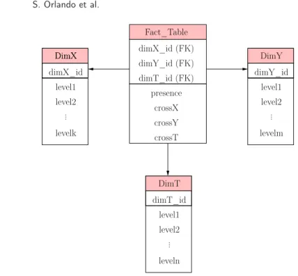
dimT_id (FK) dimY_id (FK) dimX_id (FK) presence crossX crossY crossT Fact_Table DimX dimX_id DimX level2 DimT dimT_id level1 level2 DimY dimY_id level1 level1 level2 levelk ... ... ... levelm leveln
Figure 4. The Trajectory DW model.
have a portable software, we also tested alternative implementations which employ standard SQL.
Let us first describe the data model for our TDW, illustrated in Figure 4. As presented in Section 4, we define three dimension tables, two for the spatial dimen-sion, DimX and DimY, ranging over equally sized spatial intervals, and one for the temporal dimension,DimT, ranging over equally sized temporal intervals. For each base intervalIin each dimension, the corresponding table contains its identifier and some attributes level1, level2, . . . , modelling a set-grouping hierarchy, defined by the user. In particular, attributelevelj assumes as value the identifier of the interval at the j-th level of the hierarchy includingI. Referring to the simple hier-archy shown in Figure 1(c), ifI="[60,90)", the corresponding attributelevel1
contains the father of I in the hierarchy, i.e. "[60,120)". The Fact_Table has the conjunction of the foreign keys of the dimension tables, (dimX_id, dimY_id,
dimT_id) as primary key, andpresence,crossX,crossYandcrossTas measures. Since in this paper we focus on the measurePresence, the other measures, such as distance andaverage speed, are not reported in the figure.
As already remarked in Section 4, the fact table contains only aggregate infor-mation about trajectories (i.e., the number of distinct trajectories in a cell and the number of distinct trajectories crossing the X, Y and T border of the cell). The identifiers of the trajectories and their observations are not kept in the TDW. These data can be stored into a Moving Object Database (MOD) [Güting and Schneider 2005], which can be useful also to extract higher level knowledge that in turn will feed the TDW. In this context, the features of a spatial Database, like Spatial Oracle, could be of great help for storing, querying and indexing trajectories (see Journal of Computing Science and Engineering, Vol. 1, No. 2, December 2007
e.g. [Pelekis et al. 2006]). In this paper, we focus only on the design of the TDW while issues related to the MOD are not of interest.
7.1 The ETL process
In our prototype we assume that data arrive in streams of observations of the form
(id, t, x, y), ordered by time, and we extract an observation at a time from this ordered stream.
In thetransformationphase we prepare data for loading. In particular, we trans-form the various observations into single contributions to the measures to be stored in the various cells. Then such contributions must be grouped-by, in order toload the actual final measures into the DW cells.
The main operations of our transformation phase consist of:
(i) transforming each observation(id, t, x, y)into acell tuple, containing thekey of the corresponding base cell into which the observation falls into, and its contri-bution to the cell measures;
(ii) determining, through linear interpolation, the base cells traversed by a trajec-tory where no observation falls, and creating the relative cell tuples;
(iii) avoiding the production of duplicate contributions to the same cell for the same trajectory. Therefore, if the current observation of a trajectory falls into the same base cell of the last received point for the same trajectory, we avoid producing a cell tuple.
Finally, during the loading phase of the cell tuples obtained by the previous procedure, another transformation operation is necessary to obtain the measures to store in a cell:
(iv) aggregating the cell tuples according to the cell key, and summing up the corresponding measures, thus resulting into a single tuple for each cell traversed by at least one trajectory. This tuple corresponds to the base cell to insert into the TDW.
It is worth remarking that, in order to obtain a correct update of our TDW, this loading procedure must occur at fixed times. In particular, if∆T is the temporal granularity of the base cells of the TDW, we can load the tuple cells that have been so far produced when all the observations that fall in a given ∆T interval (or a multiple of ∆T) have been received and transformed. All the tuple cells grouped-by and loaded in the TDW have to refer to this∆T interval (or a multiple of∆T).
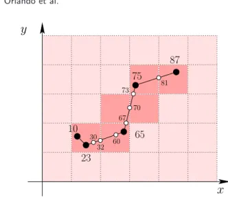
Let us give an example of the result of the transformation process. Consider the set of observations depicted in Figure 1(a). Then, we reconstruct the whole trajec-tory by using linear interpolation, as discussed in Section 3. Figure 5 shows the re-constructed trajectory together with the discretized 2D space and the points where the interpolated trajectory intersects the spatio-temporal cells. The transformation phase generates thecell tuples described in Table I where (dimX_id, dimY_id, dimT_id) – i.e., the conjunction of the foreign keys for theX, Y, and T dimen-sions – is the primary key for the fact table of our TDW1. The observation with 1For the sake of clarity, we use the corresponding intervals instead of the numeric values of such Journal of Computing Science and Engineering, Vol. 1, No. 2, December 2007
x
10 75 65 23 87y
30 32 60 67 81 70 73Figure 5. Linear interpolation of a 2D trajectory. The white points correspond to intersections between the interpolated trajectory and spatial/temporal borders.
Table I. The cell tuples obtained by the transformation phase. For the sake of clarity, we also report the timestamps (labels) of the original (or interpolated) points shown in Figure 5 that originated each tuple. Note that some points, like the one labelled by23, may not correspond to any tuple: this avoid counting duplicates in the DW.
Tstamp dimX_id dimY_id dimT_id presence crossX crossY crossT
10 [30,60) [30,60) [0,30) 1 0 0 0 30 [30,60) [30,60) [0,30) 0 0 0 1 32 [30,60) [30,60) [30,60) 1 1 0 0 60 [60,90) [30,60) [30,60) 1 0 0 1 65 [60,90) [30,60) [60,90) 1 0 0 0 67 [60,90) [30,60) [60,90) 0 0 1 0 70 [60,90) [60,90) [60,90) 1 1 0 0 73 [90,120) [60,90) [60,90) 1 0 1 0 75 [90,120) [90,120) [60,90) 1 0 0 0 81 [90,120) [90,120) [60,90) 0 1 0 0 87 [120,150) [90,120) [60,90) 1 0 0 0 timestamp10 generates the first tuple, whereas no tuple is created by the second observation (timestamp23) since it is inside the same cell of the first point. The second, the third and the fourth tuples are inserted because the interpolated tra-jectory between the observations with timestamp23and 65crosses a T border, a
X border and a T border, respectively, of spatio-temporal base cells. Note that, by construction, in each tuple cell the measures can assume only the values0or1, since we process each single trajectory in isolation. Therefore we can have different cell tuples having the same value for the primary key. Only when we aggregate
foreign keys.
Table II. Performances of the loading techniques
Method rows per second
SQL*Loader 26695
INSERT 1446
INSERTBatch 4135
EXTERNALTable 30884
MERGE INTO 4834
these cells according to(dimX_id, dimY_id, dimT_id), we obtain a unique tuple containing the actual values to be loaded into the fact table.
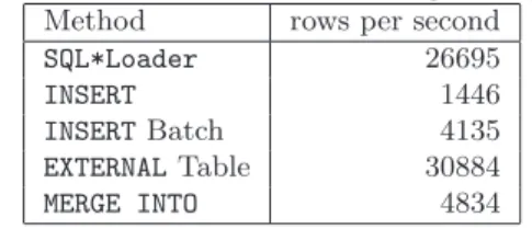
7.1.0.1 Transformation/Loading Tools.. In order to feed the DW, we analysed different techniques:
—SQL*Loader: this is the standard loading tool for Oracle. It is a command line
tool that can refresh the data in the DBMS. A configuration file describes the format of data in the input file and how these data are loaded into a DBMS table.
—SQLINSERT: this is a common way to process and load data by using an external ad-hoc application, which can exploit an API for Database Connectivity (e.g., JDBC for Java applications) to load data. It can perform whichever operations, and it has complete control on the operations to perform on importing data.
—batch SQL INSERT: as the above, but optimised for large number of insertions (the insertions are executed in blocks for optimising the performance).
—EXTERNALTable: this is a way for accessing external data from within the DBMS,
which can operate on external text files in the same way as DBMS tables. To use
EXTERNALTable as a transformation/loading tool, consider that we can perform any SQL transformation on external tables, and copy the results of these SQL queries into the DBMS internal tables.
—MERGE INTO: this is the Oracle tool for updating a DBMS table from other tables,
or evenEXTERNALones. Each single row of the DBMS table can be updated or inserted, depending on a Boolean condition.
We compared the above solutions to load the TDW, using an enlarged version (151k trajectories) of the Tiger dataset described in Section 6.2. The results ob-tained, expressed in terms of maximum throughput, are reported in Table II. It turns out that the fastest way of importing data is throughEXTERNALTables.
7.1.0.2 Implementing the ETL process.. Even if EXTERNALTables allow us also to make whichever SQL manipulations on the data during the import, for perfor-mance reasons, we decided to implement the most complex transformations, such as interpolation and the computation of the contribution of each observation to the measures, by using a Java application. This Java application is also in charge of extracting the observations from the incoming stream.
In summary, our ETL process works as follows:
—a Java application reads, one at a time, the trajectory observations from the temporally-ordered stream of observations. For each observation, it retrieves from an internal buffer the previous observation of the same trajectory, and Journal of Computing Science and Engineering, Vol. 1, No. 2, December 2007
checks whether the current observation falls in the same base cell of the stored one. If it belongs to a different cell (or, it is the first read observation of a given trajectory), our application determines its contribution to the cell measures, and creates a new cell tuple (like the ones shown in Table I) that is appended to a temporary file. Moreover, it computes other possible cells traversed by the trajectory via interpolation, also appending the correspondingcell tuples to the temporary file (operations(i)–(ii)–(iii) of the transformation stage).
As mentioned above, to simplify the following phase and avoid errors while load-ing the DW, multiple temporary files are created/updated by our application. More precisely, all the cell tuples that fall into a given interval ∆T of the time dimension of our DW, are appended to the same file.
—Each completed temporary file can be viewed by the DBMS as an External
Table. The cell tuples are thus aggregated via aGROUP BYcommand, according to the primary key of the cell (dimX_id, dimY_id, dimT_id), and the measures are simply summed up. In this way, we prepare a single/distinct tuple for each cell (operation (iv) of the transformation stage). The resulting tuples can be simply inserted into the fact table of the DW, and, finally, the temporary file can be thrown away.
We chose this distribution of the ETL task between the Java application and the DBMS also to keep the amount of memory used by the Java application low: we only need a buffer containing, for each trajectory, the last processed observation, whereas the cell tuples with the measures are directly appended to a temporary file. In this way, we do not need to maintain in the main memory all the contributions to the measures to store in the various base cells of our TDW.
We tested the ETL implementation we have discussed so far, by using the Tiger dataset. It took 27 minutes to load all the 151000 trajectories (10867722 observa-tions) of the dataset. We also tested other ETL implementations, based on either SQL INSERT or MERGE INTO. They required about 6 hours to complete. 7.2 Aggregation
The challenging problem concerning aggregation is due to the measure presence. As discussed in Section 5.1, we compute the value of this measure, for the higher levels of the hierarchy, by using two approximate functions, one distributive and the other one algebraic. The implementation of the distributive function is based on the aggregate standard function SUM applied to the measure presence. Then, by using the CUBE operation we can summarise between multiple dimensions. For instance, givenlevelIas the layer of the hierarchy on dimensionX,levelHas the layer of the hierarchy on dimensionY andlevelJas the layer of the hierarchy on dimensionT, we can obtain an aggregate information for all the combinations of these three levels, i.e.,23 groupings. The SQL query is the following:
SELECT dt.levelI, dX.levelH, dY.levelJ, SUM(presence) FROM Fact_Table ft, DimT dt, DimX dX, DimY dY WHERE ft.dimT_id = dt.dimT_id AND ft.dimX_id= dX.dimX_id AND
ft.dimY_id=dY.dimY_id
GROUP BY CUBE (dt.levelI, dX.levelH, dY.levelJ);
The implementation of the algebraic function is more complex since it requires the combination of several aggregate functions and the use of a non-standard SQL operation. In fact, suppose that we want to roll-up n adjacent cells along the X
dimension. We have to implement the following operation:
Σn−1
i=0Cx+i,y,t.presence−Σin=0−2Cx+i,y,t.crossX
The difficulty consists in avoiding to subtract the crossX of the last cell of this sequence of cells. In fact, considering the sequence of cells as a single cuboid, the presence in it is given by the sum of the presence in each cell corrected by removing the flow (i.e., the number of crossing trajectories) at the internal X borders. In Oracle, theLAST function is available: it operates on a set of values from a set of rows that rank as thelast with respect to a given sorting specification. As for the above query, we use theCUBE operation to obtain all the possible combinations.
SELECT dt.levelI, dX.levelH, dY.levelJ,
SUM(presence)-(SUM(crossX)+SUM(crossY)+SUM(crossT))+ (SUM(crossT) KEEP (DENSE_RANK LAST ORDER BY dimT_id ASC) + SUM(crossX) KEEP (DENSE_RANK LAST ORDER BY dimX_id ASC) + SUM(crossY) KEEP
(DENSE_RANK LAST ORDER BY dimY_id ASC)) FROM Fact_Table ft, DimT dt, DimX dX, DimY dY WHERE ft.dimT_id = dt.dimT_id AND ft.dimX_id= dX.dimX_id AND
ft.dimY_id=dY.dimY_id
GROUP BY CUBE (dt.levelI, dX.levelH, dY.levelJ);
The constructKEEP. . .DENSE_RANK LASTindicates that the aggregation will be ex-ecuted over only those rows havingmaximumdense rank. This construct simplifies the computation of the algebraic function for the presence. In fact, a solution withoutLASTwould require several nested queries combined with the use of outer joins.
As far as the performance is concerned, the first query has an execution time less than the second one, as expected. However, the difference is around30%.
8. CONCLUSIONS
In this paper we discussed some relevant issues arising in the design of a DW devised to store measures regarding trajectories. In particular, we focused on the research problems related to storing and aggregating the holistic measure presence. We contributed a novel way to compute such a measure in an approximate, but nevertheless very accurate way. We also compared our approximate function with the method proposed in [Tao et al. 2004], based on sketches, showing, with the help of various experiments, that in our case the error is in general much smaller.
We also analysed the design issues deriving from the implementation of an Oracle prototype of our TDW. We have investigated in depth its feasibility, and, in partic-ular, the challenges deriving from the ETL process of the DW, which has to start from a stream of trajectory observations, possibly produced at different rates, and arriving in an unpredictable and unbounded way. In addition, we have analysed the issue related to the computation of our approximate aggregate functions, used to roll-up on the presence measure.
Acknowledgements: We thank the researchers involved in the EU Project GeoP-KDD for many fruitful discussions and suggestions. This work has been partially supported by the FP6-14915 IST/FET Project GeoPKDD funded by the European Union.
REFERENCES
Braz, F.,Orlando, S.,Orsini, R.,Raffaetà, A.,Roncato, A.,and Silvestri, C.2007. Approximate Aggregations in Trajectory Data Warehouses. InSTDM Workshop. 536–545.
Brinkhoff, T.2002. A Framework for Generating Network-Based Moving Objects. GeoInfor-matica 6,2, 153–180.
Chaudhuri, S. and Dayal, U.1997. An overview of data warehousing and OLAP technology. InSIGMOD Record. Vol. 30. 65–74.
Damiani, M. L. and Spaccapietra, S.2006. Spatial Data Warehouse Modelling. Processing and Managing Complex Data for Decision Support. 21–27.
Flajolet, P. and Martin, G.1985. Probabilistic counting algorithms for data base applications. Journal of Computer and System Sciences 31,2, 182–209.
Frentzos, E., Gratsias, K.,Pelekis, N., and Theodoridis, Y. 2005. Nearest Neighbor Search on Moving Object Trajectories. InSSTD’05. 328–345.
Gray, J.,Chaudhuri, S.,Bosworth, A.,Layman, A.,Reichart, D.,Venkatrao, M., Pel-low, F.,and Pirahesh, H.1997. Data cube: A relational aggregation operator generalizing group-by, cross-tab and sub-totals.DMKD 1,1, 29–54.
Güting, R. H.,Boehlen, M. H.,Erwig, M.,Jensen, C. S.,Lorentzos, N. A.,Schneider, M.,and Vazirgiannis, M.2000. A foundation for representing and quering moving objects. ACM TODS 25,1, 1–42.
Güting, R. H. and Schneider, M.2005. Moving Object Databases. Morgan Kaufman.
Han, J., Chen, Y.,Dong, G., Pei, J.,Wah, B. W.,Wang, J., and Cai, Y. D. 2005. Stream Cube: An Architecture for Multi-Dimensional Analysis of Data Streams. Distributed and Parallel Databases 18,2, 173–197.
Han, J., Stefanovic, N.,and Kopersky, K. 1998. Selective materialization: An efficient method for spatial data cube construction. InPAKDD’98. 144–158.
Kollios, G.,Gunopulos, D., and Tsotras, V. J.1999. On indexing mobile objects. In PODS’99. 261–272.
Lopez, I.,Snodgrass, R., and Moon, B.2005. Spatiotemporal aggregate computation: A survey. IEEE TKDE 17,2, 271–286.
Papadias, D., Tao, Y.,Kalnis, P.,and Zhang, J. 2002. Indexing Spatio-Temporal Data Warehouses. InICDE’02. 166–175.
Pedersen, T. and Tryfona, N.2001. Pre-aggregation in Spatial Data Warehouses. InSSTD’01. LNCS, vol. 2121. 460–480.
Pelekis, N.,Theodoridis, Y.,Vosinakis, S.,and Panayiotopoulos, T.2006. Hermes – a framework for location-based data management. InEDBT’06. 1130–1134.
Pfoser, D.,Jensen, C. S.,and Theodoridis, Y.2000. Novel Approaches in Query Processing for Moving Object Trajectories. InVLDB’00. 395–406.
Sistla, A., Wolfson, O., Chamberlain, S., and Dao, S. 1997. Modeling and Querying Moving Objects. InICDE’97. 422–432.
Tao, Y.,Kollios, G.,Considine, J.,Li, F.,and Papadias, D.2004. Spatio-Temporal Ag-gregation Using Sketches. InICDE’04. 214–225.
Tao, Y. and Papadias, D.2005. Historical spatio-temporal aggregation.ACM TOIS 23, 61–102.
Vitter, J. S.,Wang, M.,and Iyer, B.1998. Data Cube Approximation and Histograms via Wavelets. InCIKM’98. ACM, 96–104.