Radio Frequency Traffic Classification over WLAN
Joe Kornycky, Omar Abdul-Hameed, Ahmet Kondoz, and Brian C. Barber
Abstract—Network traffic classification is the process of analysing traffic flows and associating them to different categories of network applications. Network traffic classification represents an essential task in the whole chain of network security. Some of the most important and widely spread applications of traffic classification are the ability to classify encrypted traffic, the iden-tification of malicious traffic flows and the enforcement of security policies on the use of different applications. Passively monitoring a network utilising low-cost and low-complexity Wireless Local Area Network (WLAN) devices is desirable. Mobile devices can be used or existing office desktops can be temporarily utilised when their computational load is low. This reduces the burden on existing network hardware. The aim of this paper is to investigate traffic classification techniques for wireless communications. To aid with intrusion detection, the key goal is to passively monitor and classify different traffic types over WLAN to ensure that network security policies are adhered to.
Classification of encrypted WLAN data poses some unique challenges not normally encountered in wired traffic. WLAN traffic is analysed for features that are then used as an input to six different Machine Learning (ML) algorithms for traffic classification. One of these algorithms (a Gaussian mixture model incorporating a universal background model) has not been applied to wired or wireless network classification before. The authors also propose a ML algorithm that makes use of the well-known vector quantisation algorithm in conjunction with a decision tree - referred to as a TRee Adaptive Parallel Vector Quantiser (TRAP-VQ). This algorithm has a number of advantages over the other ML algorithms tested and is suited to wireless traffic classification. An average F-score (harmonic mean of precision and recall)>0.84was achieved when training and testing on the same day across six distinct traffic types.
Index Terms—Traffic Classification, Machine Learning, WLAN, Wi-Fi.
I. INTRODUCTION
I
N the modern age, the use of encryption in communication systems is becoming ever more common. With the intro-duction of Long Term Evolution (LTE), cellular networks are moving away from conventional circuit-switched voice and are utilising Internet Protocol (IP) data packets to carry this data. Voice over Internet Protocol (VoIP) is more prevalent due to it offering greater transmission efficiency and allowing more users in the same bandwidth.For WLAN, the use of IP means that there is a wide variety of encryption algorithms that could be used. In many situations, this data could be encrypted at the IP layer and then encrypted (possibly with a completely different encryption algorithm) again when it is passed over a WLAN. When monitoring a wireless network for unauthorised users, it is generally not possible to perform real-time decryption at
J. Kornycky & B.C. Barber are with Defence Science and Technology Laboratory (Dstl), Porton Down, UK. (see http://www.dstl.gov.uk)
O. Abdul-Hameed and A. Kondoz are with Loughborough University London, UK
Manuscript received May 27, 2015; revised # #, 2015.
each node of the network to check for unauthorised access. The concept of traffic analysis and classification was created to ascertain whether it is possible to identify unauthorised usage of a network purely based on features present in the encrypted data. For example, utilising the packet sizes, the packet inter-arrival times, as well as the encoding schemes to distinguish between the different types of traffic (e.g., VoIP, web browsing, or streaming video). If the traffic identified is not what is expected on the system, then there is a possibility of an intruder, for example, web browsing identified when the network should be streaming video. Note that the packet header information cannot be relied upon as it can be re-encapsulated as another form of traffic.
Traffic classification involves analysing data flows on com-munications links and identifying the type of content these flows contain. This could be coarse traffic classification that identifies the data type, for example, email, File Transfer Protocol (FTP), web browsing etc. Or fine traffic classification that also indicates which application was used, for example, (in the case of email) Thunderbird, Outlook, Gmail, or Hotmail etc. Techniques for classification of IP data are desirable for numerous other applications, such as network monitoring, QoS measurements, network planning, and intrusion detection (through the identification of abnormal/malicious data flows). Techniques for classifying Internet traffic flows can broadly be divided into three major categories: port-based approaches, Deep Packet Inspection (DPI), and statistical approaches. These approaches all still have certain limitations.
The simplest method is the Port-based approach that exam-ines, for example, Transmission Control Protocol (TCP) port numbers. Port-based approaches are more simplistic because many well-known applications are associated with specific ports, for example, Hypertext Transfer Protocol (HTTP) traffic uses port 80 and FTP traffic uses port 21. However, it is recognised that Port-based classification is inadequate [1], [2], [3], [4], because many applications use dynamic port-negotiation mechanisms to hide from firewalls and network security tools. When sent over a WLAN, these port numbers are typically encrypted as they do not form part of the typical encrypted WLAN protocols. This makes analysis of WLAN data ever more challenging.
Approaches based on DPI are usually considered very reli-able for traffic that is not encapsulated into other application-level protocols and for unencrypted traffic. However, the current trends show that the portion of encrypted traffic on the Internet is constantly increasing [5], and many applications are using protocol encapsulation or obfuscation to evade network policy enforced through filtering [1]. In addition, access to the full payload is often not possible (e.g., due to privacy or performance issues).
packet size or Inter-Arrival Time (IAT) over groups of packets. Machine Learning (ML) algorithms are then used to classify traffic based on statistical attributes in these features.
Many large firms are making use of passive monitoring devices to analyse WLAN [6], [7]. These monitoring devices can be loaded onto mobile platforms and even existing office desktops can be converted (using a WLAN dongle) to carry out analysis when local computational load is low [8]. Existing Access Points (APs) and network hardware can be used but this puts extra strain on the existing network architecture. Cheap passive devices can be used to: localise rogue APs, spot rogue ad-hoc networks, help disconnected clients, monitor network performance, detect Denial of Service (DOS) attacks, find optimal hand-offs between APs, and recover from mal-functioning APs. Improving network monitoring services is highly important for large corporations where secure wireless infrastructure is vast. For example, MicrosoftTMutilise approx-imately 5000 APs, for over 25,000 users, in 277 buildings, covering approximately 1 million square feet [8].
This paper investigates the use of low cost WLAN dongles to passively monitor a network and perform traffic classifica-tion. The concept here is to improve the monitoring services available to a network for either security or analysis of net-work performance. We focus on the application of enforcing network security policies by identifying allowed/disallowed WLAN traffic types. We draw together ideas from two fields: low cost passive monitoring and statistical traffic classification. It would be unrealistic, from a security perspective, to share decryption keys for all APs with passive monitoring devices. Hence, analysis is performed on encrypted WLAN data. Previ-ous work, in the traffic classification field, had either: utilised unencrypted WLAN, obtained features from wired portions of the network where higher layer IP information was available [9], or solely monitored for Wi-Fi specific attacks. As the data is encrypted, port numbers, DPI and flow-level analysis cannot be exploited here.
The contributions of this paper are:
• The creation of a large data set that contains data from multiple days, using multiple traffic types (email, FTP, web browsing, Voice over Internet Protocol (VoIP), and video), and uses multiple applications.
• Analysis of 63 features derived from statistics based on uplink/downlink packet length and IAT.
• Six different ML algorithms were applied to the data in-cluding K Nearest Neighbour (KNN), Weighted KNN, a Gaussian Mixture Model (GMM), a GMM incorporating a Universal Background Model, a Binary Classification Tree (BCT), and a Parallel Tree Structured Vector Quan-tiser (PTSVQ).
• Additionally, an ML algorithm is proposed that makes use of the well-known vector quantisation algorithm in conjunction with a decision tree, referred to as a TRee Adaptive Parallel Vector Quantiser (TRAP-VQ).
• An F-score>0.84when training and testing on the same day and >0.60 when training and testing on data from different days was achieved using TRAP-VQ.
• We also utilise a pre-classification stage to further im-prove the cross-day classification performance. This stage
identifies which training data set best matches the condi-tions of the testing data. This increases the worst cross-day F-score from0.60to0.66.
The remainder of this paper is organised as follows. In the next section, we provide an overview of traffic analysis and classification algorithms as well as related work. Section III provides our experimental WLAN test-bed setup and the data set collection. In section V, we present feature collation, extraction, and selection. Section VI presents the machine learning algorithms used. Section VII presents the results obtained and analyses the performance. Finally, the paper is concluded in section VIII.
II. RELATEDWORK
In the previous section, we highlighted the need to move away from port and DPI based approaches and focus on statis-tical methods of traffic classification. In traditional traffic clas-sification this is due to many applications using unpredictable port numbers and encrypting or modifying data payloads to prevent DPI. Even when ignoring security/encryption issues and focusing on QoS applications of traffic classification, techniques not reliant on packet contents are advantageous due to the many issues highlighted with Integrated Services (IntServ) [10] and Differentiated Services (DiffServ) [11] based QoS management. Past papers in this area have made use of ML algorithms to classify statistical features in the data. These algorithms are generally utilised in two phases: the training phase and the testing phase. In the training phase, features are extracted from a particular traffic type. These features are typically values calculated over multiple packets, e.g., maximum packet length or mean packet IAT. Features can be extracted from all packets in a flow or simply from packets flowing in one direction (i.e., directionality can be incorporated as a feature [12]). Features from multiple different traffic types are then used to train an ML algorithm. The flows are either analysed in their entirety or further broken down into sub-flows using a sliding window for analysis, e.g., split the data into 0.5 second windows and calculate the features in each window. In the testing phase, when a new traffic flow appears on the network, statistical features can be extracted and the aforementioned ML algorithm can then attempt to identify what type of traffic is present.
One of the first papers in this area used expectation max-imisation to classify wired network traffic into three generic traffic categories (bulk transfer, small transactions and multiple transactions) [13]. Since then many papers have attempted to analyse traffic types and perform coarse (identifying traffic type) and/or fine (also identifying the application used) traffic classification using a variety of techniques:
a) Nearest Neighbour: Where a decision is made on a testing point’s assignment based on its proximity to neighbour-ing points in the trainneighbour-ing data [14], [15].
b) Clustering approaches: k-means [16], Density-based spatial clustering (DB-SCAN) [16], subspace clustering [17]. c) Discriminant analysis: Linear Discriminant Analysis (LDA) [14], Quadratic Discriminant Analysis (QDA) [14], Support Vector Machines [18].
d) Probabilistic techniques: Maximum Likelihood esti-mation [19], regularised maximum entropy [20], Naive Bayes [21], AutoClass [16], Bayesian network [22], Bayesian Neural network [23].
e) Decision Trees: basic decision trees [24], [25], Deci-sion Tree J48 [26], Reduced error pruning [26], C4.5 deciDeci-sion tree [22], [27], Random Forest Decision Tree [28], Context Tree Weighting (CTW) [28].
f) Neural Networks: Artificial Neural Network (ANN)[25], Flexible Neural Tree (FNT) [29], Radial Basis Function Neural Network (RBFNN) [30], Multilayer perceptron [30].
g) Genetic algorithms: Sequential Forward Selection (SFS) [31], Symbiotic bid-based genetic programming [32], Multi-Objective Genetic Algorithm [33].
h) Miscellaneous: Pearson’s Chi-Squared test [34], Lo-gistic regression model [35], Adaboost [20], score level fu-sion using multiple implementations of the LindeBuzoGray (LBG)+Splitting algorithm [36].
In many of the papers mentioned above, TCP port numbers or values extracted from DPI were included as features to be passed to ML algorithms. Therefore, if available, they would be used as features alongside statistics based on packet length, IAT etc. Our specific application of WLAN monitoring precludes the use of port numbers and DPI; therefore we only use features based on packet length and IAT. While techniques exist to modify packet length and IAT to circumvent traffic analysis [37], these techniques incur significant overheads (in terms of processing and latency) and are hence not investigated here.
Previous work in this area was also able to break traffic types up into a series of smaller flows (by analysing forward-ing addresses and dead periods or breaks in the traffic). As forwarding information is not available here, we do not make this distinction, and flow-level statistics are not utilised. In a network security application of traffic classification where decisions need to be made as packets come into the system, knowing that a flow was malicious or against network policy after it has traversed the network is not useful, i.e., classifica-tion should be timely and continuous [38].
III. DATASET
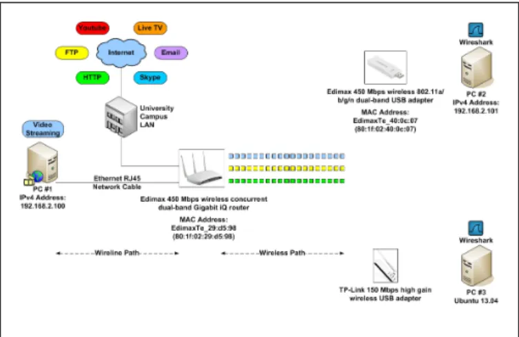
In this section, we present the developed experimental WLAN test-bed and the measurement tools and techniques that were used for capturing the data set. Basic WLAN architecture generally consists of an Access Point (AP) and one or more remote devices (clients) that connect to the AP over radio links. The AP generally connects to a wired network (e.g., an xDSL link), acting as a gateway point between the wired network and the wireless network and it is commonly Internet enabled. The architecture of the experimental test-bed used in this paper is illustrated in Figure 1. PC #1 was provided with a WLAN router/AP, which was an Edimax (BR-6675nD) 450 Mbps wireless concurrent dual-band Gigabit iQ router, forming the indoor infrastructure WLAN. The WLAN wireless router/AP was connected to a University Campus Local Area Network (LAN), which in turn had provided the connectivity to the Internet.
Fig. 1. Experimental WLAN test-bed architecture
At PC #1, a number of different applications were provided, such as video streaming, FTP, web browsing, email, and Skype. PC #2 was provided with a WLAN USB adapter, which was an Edimax (EW-7733UnD) 450 Mbps wireless 802.11a/b/g/n dual-band USB adapter. This was used for collecting the decrypted version of the transmitted traffic over the setup WLAN network for reference purposes. In addition, PC #2 ran the Wireshark [39] tool for monitoring and collection of the measurements. PC #3 running Ubuntu 13.04 was provided with a WLAN USB adapter, which was a TP-Link (TL-WN722N) 150 Mbps high gain wireless USB adapter. This was used to capture all the encrypted traffic that was transmitted over the WLAN network. In addition, PC #3 ran the Wireshark tool to capture all the encrypted traffic.
In this work, six popular Internet applications were used to generate the Internet traffic data set. The data set included different traffic types: video streaming, FTP, web browsing, email (using a client), email (using a web browser), and VoIP using Skype. In addition, each of the aforementioned traffic types was collected with different variations. For example, the most popular web browsers were utilised in the data set collec-tion, including Internet Explorer, Firefox, Safari, and Chrome. Table I lists the Internet applications that were used for the data set. The data set was constructed by collecting the traffic of the different considered Internet applications on four different days, where each day had included the collection of traffic that was generated by each of the considered applications. Table II shows how the data set was constructed.
The Video Streaming traffic data set collection was con-ducted using the Darwin Streaming Server (DSS) RTP/RTSP server that was running at PC #1 and the Apple QuickTime 7 client that was running at PC #2. Four video test sequences with different image resolutions and motion characteristics were used. Each raw video test sequence was compressed offline using the H.264/MPEG-4 AVC reference software [40]. Each compressed video test sequence was then encapsulated into an MP4 encapsulation format for transmission using the DSS server. The FTP traffic was collected in two different ways. The first was web-based, i.e., using the four different Internet browsers. The second was using FileZilla [41] Server
TABLE I
LIST OFINTERNET APPLICATIONS USED
Application Name / Traffic Type
Software Server/ Website/ Varia-tions
Video streaming Darwin Stream-ing Server and Quicktime
Different video test se-quences
FTP Internet Explorer, Firefox, Safari, Chrome, Filezilla
Different FTP servers
Web browsing Internet Explorer, Firefox, Safari, Chrome
Browsing through differ-ent websites
Web based email Internet Explorer, Firefox, Safari, Chrome http://www.hotmail.com Client based email Thunderbird https://www.mozilla.org/en-GB/thunderbird/
Skype / VoIP Skype Different Skype conversa-tions
TABLE II DATA SET CONSTRUCTION
Day # 1 2 3 4
Date 23/09/13 10/10/13 23/10/13 20/03/14
Day Mon Thur Wed Thur
Classes collected: (thousands of packets)
Client based emailing 30 32 32 69
FTP 154 390 77 114
Skype / VoIP 239 335 291 93
Video streaming 2 24 23 27
Web browsing 96 78 105 125
Web based email 1.4 1.2 1.4 1.9
(FileZilla Server-0.9.41) and Client (FileZilla 3.6.0. 2), which is an open source free FTP software solution. The Web Browsing traffic was generated by browsing different websites with different content using the four different Internet browsers for durations of 3 to 5 minutes each. For the Email traffic, two types of Email were considered in the data set collection, including web-based email using the four different Internet browsers and client-based email using Mozilla Thunderbird [42]. Skype is a popular proprietary Voice over IP (VoIP) Internet application that allows making voice/video telephone calls over the Internet. Skype normally uses a Sinusoidal Voice Over Packet Coder (SVOPC). Skype traffic was used for collecting voice only, video only, and voice and video traffic combinations with each session lasting for 5 minutes.
IV. DATASETANALYSIS
The first step in analysing the captured wireless trace files was to extract or filter the desired conversation traffic from the many other conversations that were captured both from the target WLAN and other University WLAN devices operating in the same area. In addition, the aim of this step was to investigate whether there were features that could be extracted from the Radio Frequency (RF) domain over a WLAN wireless network and whether such features could be utilised effectively
for the purpose of classifying the different types of traffic being carried over a WLAN network.
In the unencrypted domain, features for traffic classification can be obtained from the packet headers in the TCP/UDP and the IP layers, such as the TCP/UDP port numbers, IP addresses, payload information, etc. However, in the encrypted domain, where the WLAN MAC-layer frames are usually en-crypted, the available information is very limited. Such limited information from the MAC header could only include the MAC address, Service Set Identifier (SSID), traffic direction (uplink or downlink), RF signal strength, and the frame types. In addition, it is only possible to get the packet lengths, packet timestamps, and the packet inter-arrival times.
The desired traffic conversations were filtered from the many other conversations that were captured over the tar-get WLAN network and other University WLAN devices operating in the same area by utilising the un-encrypted Source/Destination 6-byte MAC address parameter. Upon filtering the desired traffic conversation for each captured session, the second step was to analyse each individual traffic type in terms of its average Frame or Packet Length/Capture Length and average Frame or Packet Inter-Arrival Time (IAT) characteristics, which were obtained using the Wireshark tool, in order to get an insight into its features and behaviour. For example, the Frame Length/Capture Length and the Frame inter-arrival Time features could be used to get an insight into the type of traffic, since different traffic types use different packet sizes and hence different Frame Lengths and also different inter-arrival times.
V. FEATURECOLLATION
The filtered (based on MAC address) Wireshark capture files were exported into MATLABTMfor analysis. From this data, features were extracted and used to train various ML algo-rithms. The Wi-Fi data was encrypted and therefore only basic information on the data was available in addition to the access point’s and user’s MAC addresses. Only the MAC addresses were used to filter the data. As the data was encrypted, non-flow specific packets (e.g., network management etc.) were also included in the data. This was done to make the system as realistic as possible. Two key attributes were utilised by the ML algorithms in order to perform traffic classification:
• Packet length, measured in number of bytes, defined as the captured packet length that was obtained from analysing the captured Wireshark traces.
• Packet Inter-Arrival Time (IAT), measured in seconds, defined as the time between the arrival of two consecu-tive packets. Measured by analysing captured Wireshark traces.
The data was put into windows of 0.5 seconds with an 80% overlap. Through experimentation with the training data, 0.5 second windows were found to give better classification performance than other sizes. An 80% overlap was used as some classes had minimal amounts of traffic flowing; hence, a large overlap was used to increase the effective amount of feature vectors and further improve the performance of the classifiers.
Analysis of the WLAN traffic showed a vast difference in the statistics between the uplink and downlink. Therefore, uplink and downlink features were calculated separately. In each window, for the two main features mentioned above, 10 different statistics were calculated in the uplink and downlink directions, refer to Table III. All permutations were calculated, so that 10 different statistics were calculated for 3 different directional flows (uplink, downlink and ratio of uplink versus downlink) for each of the 2 input measurements. 3 extra features were calculated based on number of packets in the uplink and downlink in each window. Hence, (10 statistics x 3 directional flows x 2 input measurements) + 3 extra features = 63 features. For example, some of the resulting features were: Kurtosis of the downlink packet length, mean of the uplink packet inter-arrival time, ratio of uplink-to-downlink Kurtosis of packet length etc.
This yielded a total of 63 features for analysis. It was reasoned that statistics, such as Kurtosis, skew, and variance would highlight that variation within a window as a traffic flow was set-up or highlight the variation in the flow itself. For example, during the set-up and initialisation of a VoIP call, the size of the packets would increase over time to enable transmission of video and audio. This would cause a skew in the packet size data as an observation window is slid through the captured data.
Although the data set contained Wireshark traces from multiple days, to keep these experiments realistic, only a single day’s worth of traces were used to train/adapt the parameters of each ML algorithm. Once trained, each ML algorithm could then be verified/tested against unused samples from the same day or tested on another day’s set of traces.
TABLE III
FEATURES EXTRACTED FROM WIRELESS TRAFFIC DATA
Input measurements (2) Directional flows (3) Statistics Calculated (10)
- Packet length - Uplink - Mean - Packet inter-arrival time - Downlink - Median - Ratio (uplink / downlink) - Mode - Standard deviation - Maximum - Minimum - Range - Skew - Kurtosis - Sum Extra Features (3)
- Number of uplink packets - Number of downlink packets
- Ratio of number of uplink-to-downlink packets
The raw feature vector in the uplink direction is denoted by ru(p, n), wherepandnare used to address thepth packet in the nth window. Similarly, rd(p, n) denotes the raw feature vector in the downlink direction. The resulting features were then generated by applying the appropriate function (see table
III), to the raw feature data:
x(n) = f(ru(p, n)) f(rd(p, n)) f(ru(p, n))/f(rd(p, n)) Qu(n) Qd(n) Qu(n)/Qd(n) (1)
Where Qu(n) indicates the number of uplink packets in window n,Qd(n)indicates the number of downlink packets in window n, and f is a vector of functions that has been populated by the list in the third column of Table III:
f = [fmean,fmedian...fsum]
T
(2) As an example, fmeanhas the following form:
fmean(ru(p, n)) = 1 Qu(n) Qu(n) X p=1 ru(p, n) (3)
The resulting feature vector x(n) has 63 elements and describes the statistics of each window in the uplink and downlink directions. Each of the features were centralised (by subtracting the mean), extreme outliers were removed (values outside of 5 standard deviations were removed from the training set), and the resulting data was normalised (by dividing by the largest value). Five standard deviations were chosen as the data did not have a Gaussian distribution and hence using a low number of standard deviations did not prove effective here. This method removes extreme outliers that severely affected the statistics of the data while preserving as much of the underlying distribution of the data as possible. The same mean and standard deviation found in the training phase was used in the testing phase. This meant that testing data could be analysed as a new window of features arrived into the system.
VI. MACHINELEARNING(ML) ALGORITHMS
In order to be clear on how the data was used,x(n)∈R63x1
is a generic term that describes the feature vector, whereas xtrain(n)andxtest(n)represent the portions of the data that are used for training and testing the ML algorithms. For example, day 1 could be used to creatextrain(n)and day 3 data could be used to create xtest(n) so that training and testing could be performed on data from different days. Similarly,xtrain(n) andxtest(n)could come from the same day’s worth of traces; however, they never overlapped. The following classification systems were used:
A. K Nearest Neighbour (KNN)
This system analyses each point xtest(n) separately and compares it to the K nearest points from xtrain(n) denoted by:xtrain(k1),xtrain(k2)...xtrain(kK). The classes of these neigh-bours are then analysed. The class that occurs most frequently in these neighbours is then chosen as the output class for point xtest(n).
B. Weighted K Nearest Neighbour (WKNN)
This system is very similar to KNN; however, the decision is not based on a majority vote. Instead xtrain(n) is divided up into the different classes.xtest(n)is then compared to each class withinxtrain(n)and theKnearest neighbours from each class are selected. The class with the smallest total euclidean distance between xtest(n) and its K nearest neighbours are then chosen. This method has been proven to be more effective than K Nearest Neighbour (KNN) in a variety of applications [43].
C. Gaussian Mixture Model (GMM)
A GMM is constructed based on the training data from each class separately. xtrain(n)is split into different classes and the GMM parameters are obtained using the Expectation Maximisation (EM) algorithm [44]. The GMM forms a para-metric distribution of the following form:
pc(x(n)) = L X i=1
ac,iN(x(n)|µc,i,Σc,i), (4) Where pc(x(n)) gives the probability that point x(n) be-longs to class c, L is the number of mixing components in each GMM and ac,i ≥ 0 are the component weights PL
i=1ai,c= 1
. Each Gaussian component N is charac-terised by: µc,i the multivariate component means and Σc,i the symmetric semi-positive definite component covariance matrices. A GMM is created for each class and training data from the other classes is then used to set an appropriate acceptance threshold for each of the GMMs. Throughout this paper, the Equal Error Rate (EER) was used to set the acceptance threshold. This threshold was set using only the training data. The system puts the feature vector under test through the GMM for each class to see whether its probability falls above or below the aforementioned threshold. Therefore, using this method, a single feature vector could be accepted by models from multiple classes.
D. Gaussian Mixture Model Universal Background Model (GMM-UBM)
This is the same as the GMM system; however, the prob-ability of the feature vector under test is scaled back by the probability of the point falling into a background model [44]. Throughout this paper, the background model is constructed by utilising the GMMs from all the other classes aside from the one under test:
log(pc=t(x(n))− X c6=t
log(pc(x(n))) (5)
Wheretindicates the class currently being focused on. Hence, if there is a component of feature vectorx(n)that gives rise to a high probability in the target class and also all the other classes, it will be given a lower resultant probability than in the GMM case. To the best of our knowledge, the GMM-UBM algorithm has not been used to classify wireless or wired traffic data before.
E. Binary Classification Tree (BCT)
The features in the training data are analysed and all possible binary splits are evaluated, for example, all data that has featureY ≥splitη is in one branch whereas Y < splitη is put in the other. At each node η, Gini’s Diversity Index (GDI) is used to assess the quality of the binary split dictated by splitη. Stopping criteria are met when all nodes are pure (nodes contain only data from a single class) or when all nodes contain fewer than a very small number of points. A separate tree is used for each class. This system also makes use of bootstrapping (sampling with replacement) to create multiple trees from each data set.xtest(n)is then classified by a majority vote from the ensemble of decision trees [45].
F. Parallel Tree Structured Vector Quantiser (PTSVQ) The PTSVQ algorithm can be seen as an extension of the Tree Structured Vector Quantiser, which is in turn an extension of the well-known Vector Quantiser (VQ). A VQ algorithm will attempt to represent the input data using a number of code symbols. The aim of a VQ algorithm is to find a series of code symbols that minimise the distortion between an input vector (xtrain(n)) and its representation if quantised to the location of the corresponding code symbol:
D(xtrain(n)) =||xtrain(n)−γ(xtrain(n))||2 (6) Whereγis the VQ decoding function andDis the distortion. The above is typically achieved through fast and efficient algorithms, such as the K-means algorithm. The TSVQ utilises a tree-based search method to further improve the VQ algo-rithm. The data in each branch of the tree is clustered and the distortion analysed (to begin with, all the data is used). If the decrease in the distortion is above a pre-specified value then the number of clusters is increased again. Otherwise, the clusters are dealt with separately (each cluster forms a branch in the tree structure) and another VQ algorithm is applied to each branch separately. This continues until the distortion has gone below a threshold or when there is an insufficient number of points in each branch. Therefore, the distortion in this tree structure is given by:
DMJ (xtrain(n)) = PJ
j=1 P
xtrain(n)∈cellj||xtrain(n)−m
M j ||2 N
(7) Where M represents the scale or branch number, J is the number of cells at branchM andN represents the number of observations. Therefore, ifD M J−1−D M J DM J
is above a threshold then the number of clusters is increased, otherwise more branches are formed. The PTSVQ creates a TSVQ instance for each class. During the testing phase, each data point is run through all of the TSVQ instances and assigned to the class whose model yields the smallest distortion measure.
G. TRee Adaptive Parallel Vector Quantiser (TRAP-VQ) The TRAP-VQ algorithm has been proposed in this paper and will be shown to be effective when classifying wireless network data. The other ML algorithms tested have a series
of drawbacks. Therefore, the possibility of creating a new or modified ML algorithm was investigated.
An overview of the TRAP-VQ algorithm is shown in Figure 2. Note that class(n) indicates the class of the nth point in x(n), tol is a tolerance value, target indicates the class currently being analysed, and max cells is the maximum number of cells allowed to represent the target or non-target data at each node in the tree. Initially, all the dataxtrain(n)is passed into TRAP-VQ. The testing dataxtest(n)is then passed through this tree structure and compared with the centroids at each node. Each element of the testing data is classified based on the label of the node it ends up falling into at the bottom of the tree.
H. Discussion of TRAP-VQ Versus Other ML Algorithms The TRAP-VQ algorithm was designed to require limited prior information. Other systems are reliant on users adjusting parameters, such as the number of clusters or the number of Gaussian components within GMM systems. TRAP-VQ needs to know the maximum number of allowed branches at each node, but it analyses the data and decides on an optimum number itself.
The only prior knowledge required is for the user to set the max cells value (see Section VI-G). It will be shown in the main results (Section VII) that TRAP-VQ is not sensitive to changes in this value. In fact another version of the algorithm, referred to as TRAP-VQ (bin), used a max cells value of 1 and hence creates a binary decision tree. This version of TRAP-VQ produces similar results to the main TRAP-VQ algorithm. TRAP-VQ (bin) is slightly slower to execute in the testing phase due to a larger tree structure but is significantly faster to train. Throughout this paper, tol was set to zero and hence the system will stop training when all nodes are pure. Through experimentation, analysis of the data showed that when tol was set to a higher value convergence speed in the training phase increased but the resulting error rate increased. A value of zero was chosen here to demonstrate the best performance of the algorithm.
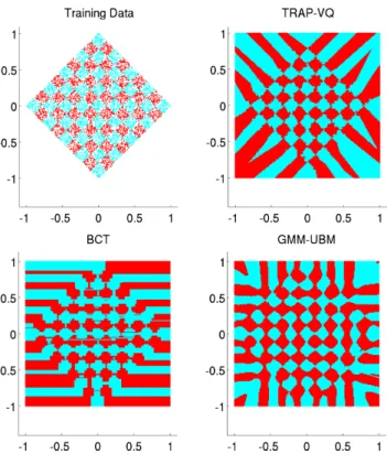
TRAP-VQ makes use of hard decision boundaries to remove the need for threshold setting (as per a GMM algorithm) and hence reduce complexity in the training phase. It makes use of the computationally efficient K-means algorithm in the training phase. If more speed is required here, this can be achieved by reducing the maximum number of centroids. Unlike the BCT, TRAP-VQ can make use of multiple features at each split in the decision tree. This means that the decision boundaries need not be parallel to the features, as shown in Figure 3.
When analysing wireless networks a vast amount of data will need to be analysed; therefore, this needs to be as simple as possible. TRAP-VQ has a similar computational complexity to a BCT or PTSVQ algorithm. It uses Euclidean distance to a series of points arranged in a tree-like structure. This is substantially faster than GMM or other probabilistic techniques, where exponential functions need to be evaluated. The BCT family of algorithms have similar advantages to TRAP-VQ; however, they can only analyse a single feature at a time. This yields decision boundaries that are potentially sub-optimal, as they must be orthogonal/parallel to the features.
Fig. 3. Fictitious two class example showing decision boundaries for different classification algorithms. Evident how TRAP-VQ can draw decision boundaries at any orientation to the feature axes, unlike BCT.
Unlike the BCT algorithm, the TRAP-VQ algorithm can draw complex decision boundaries that need not be paral-lel/orthogonal to the features.
The PTSVQ algorithm also shares many advantages with TRAP-VQ; however, PTSVQ can place decision boundaries in sub-optimal locations by training on target and non-target data separately. Unlike the PTSVQ algorithm, the TRAP-VQ algorithm utilises target and non-target data to create more optimum decision boundaries. There are of course a few disadvantages with VQ. Computationally, the TRAP-VQ algorithm is more complex in the training phase than BCT or PTSVQ based methods. However, the BCT uses multiple trees and ensemble averaging of results to improve performance. TRAP-VQ uses a single tree. The choice of ML algorithm comes down to a trade-off between performance and computational complexity in the training and testing phases. It is believed that the TRAP-VQ algorithm yields the best compromise for network traffic classification.
VII. RESULTS
This section has three subsections. In the first subsection, performance metrics for traffic classification are chosen and discussed. In the second subsection, the various features are analysed for suitability to traffic classification using Sequential Forward Selection (SFS). In the third subsection, numerous ML algorithms are applied to the WLAN traffic data and their classification performance charted.
A. Performance Metrics
There are a number of mechanisms for evaluating the per-formance of a traffic classification system or, more generally,
TRAP-VQ Algorithm- The following procedure is called on each class separately. The current class label istarget. 1) Perform Vector Quantisation (VQ) on data whose class is labelledtarget. The FINDCELLS function starts by using
single cell VQ and then increments the number of cells untilmax cellsis reached. If the total variance at the current iteration is less than5% of the total variance using only a single cell, the system stops. Otherwise, a single cell is used. µtarget is the resultant VQ encoding function.
µtarget←FINDCELLS(x(n)∈target, max cells)
2) As per step (1) but using non-target data.
µnon-target←FINDCELLS(x(n)Z∈target, max cells)
3) Combine the target and non-target centroids from steps 1 and 2 to create a new VQ encoding functionΦand ignore the target/non-target labels.
Φ←(µtarget,µnon-target)
4) For each of the cells in Φ, calculate the error in two situations: the first assuming that the cell is labelled as target (to get the number of false positives) and the second assuming a non-target label (to get number of false negatives). Whichever error rate is lower dictates the cell ID, i.e. target or non-target. If the error is above tol then the data is labelled as continue.
[error, cell ID]←CALCULATE ERROR(Φ,x(n), class(n))
5) Each cell forms a branch in a tree-like structure. The branch label (cell ID) is eithertarget,non-target, orcontinue. If target or non-target has been assigned, this branch of the tree stops. If the branch/centroid is labelled as continue, this portion of the data requires further clustering and is passed through the system again (i.e., data from this cell is used as x(n)and steps 1 to 4 are repeated).
Fig. 2. TRAP-VQ pseudocode
a ML algorithm. Typically this involves evaluating metrics, such as precision and recall. In order to explain these terms, we will assume that the system is attempting to find email traffic on a link that contains email, Internet browsing, video streaming, VoIP etc. Given this example, the following terms can be defined:
• Recall: The percentage of data that, for example, the system labels as email when in actuality it is email data. Effectively evaluates percentage of data kept by the system when only email data is fed in.
• Precision: The percentage of data that, for example, is email from all the data that the system has labelled as email. Effectively evaluates how often data labelled by the system as email is correct.
Therefore, the goal of a traffic classification system is to obtain the highest possible precision and recall. When ML algorithms are being compared across large data sets and in multiple situations a single figure is desirable. We use here the F-score:
Fβ= (1 +β2).
precision . recall
β2.precision + recall (8) F-score is defined as the harmonic mean of precision and recall [46]. This gives a value between 0 and 1. By varying the value ofβ, the relative importance of precision and recall can be traded-off. Typicallyβ is set to 1, 2 or 0.5. Throughout this paper we use F1 to evaluate the algorithms tested. This gives an even weighting to both precision and recall.
B. Sequential Forward Selection (SFS)
SFS was used to analyse all 63 features and ascertain which subset of features could be used to increase the performance. The SFS process works out the meanF1for all classes using only a single feature at a time. It then takes the feature that yielded the highest F1 and attempts to find another feature to pair it with, and so forth. The TRAP-VQ (bin) algorithm was used for the SFS tests. The F1 with each step of the SFS algorithm is shown in Table IV up to the fourth selected feature. These results show that a high F1 can be achieved with as little as two features. Day 1 and day 2 have been used for analysis, so that the remaining days can be used for testing with no prior knowledge.
The uplink maximum packet length feature is repeatedly selected as the preferred choice for the first feature in the SFS process. It should be noted that the Wi-Fi protocol acknowledgement messages were filtered out of the Wireshark traces, therefore, the uplink data represents acknowledgements and other message types from layers higher up in the protocol stack. Wireshark was also used in the wired unencrypted portion of the network so that further analysis could be carried out to understand why certain features gave rise to the smallest error rates. The main observed protocols in the uplink direction were:
• Video Streaming: RTCP, RTSP, TCP. • FTP: TCP, TLSv1, FTP.
• Web Browsing: TCP, HTTP, TLSv1. • Email: TCP, TLSv1.
TABLE IV SFSF1RESULTS
nth
Feature Feature Name F1 Precision Recall Training - day 1, Testing - day 1
1 Uplink max. IAT time 0.86 91.01 82.05 2 Uplink max. packet length 0.88 88.22 88.71 3 Downlink max. packet length 0.89 87.34 90.04 4 Ratio max. packet length 0.89 88.42 89.79 Training - day 2, Testing - day 2
1 Uplink max. IAT time 0.89 90.28 87.24 2 Uplink mode packet length 0.90 90.03 90.37 3 Ratio mode IAT time 0.90 90.00 90.28 4 Uplink min. packet length 0.90 90.97 89.40 Training - day 1, Testing - day 2
1 Uplink max packet length 0.71 70.03 71.19 2 Ratio max packet length 0.78 78.14 77.06 3 Ratio mode IAT time 0.78 78.68 76.98 4 Ratio std. IAT time 0.78 78.68 76.98
On analysis of the unencrypted Wireshark traces, it became apparent why uplink features in the encrypted data had yielded the best performance. The distributions of uplink packet size vary significantly for different traffic types, this is due to the aforementioned different protocols being used in the uplink.
In Section VII-C results are given using all 63 features as well as a down selection of 2 features - to ensure that near real-time traffic classification can be achieved, a low num-ber of features yielding significantly reduced computational complexity is important. For example, if used in a passive monitoring scenario, a low complexity system is desirable so that classification can be achieved on existing hardware without the need to upgrade or impact user performance. The two features chosen were uplink maximum packet lengthand ratio (uplink/downlink) maximum packet length . Although other feature combinations yielded a higher F1, these two features produced the lowestF1 when training and testing on different days - hence they should be more robust to day-to-day drift/variability.
C. Classification Performance Comparison
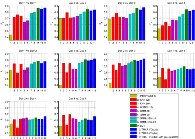
In this subsection, the various different ML algorithms reviewed in Section VII are utilised on the data set. Table V lists the algorithms and parameters used. Note also that if the training and testing data were taken from the same day, the data was divided into two non-overlapping sections. The F1 results utilising the two main features found in the previous section are shown in Figure 4. This figure gives the average F1for all traffic types (classes). In order to give an example of how the different algorithms performed against different traffic types, Table VI has been included. Note that the results for algorithm number 3 are discussed in Section VII-D.
Firstly, looking at the results when training and testing on the same day, there is a definite consistency of relative performances amongst the F1 values. The KNN and WKNN algorithms are the least computationally complex and are
TABLE V
INITIAL TESTING PARAMETERS
Parameter Value Parameter Value Algorithm 1 PTSVQ (30,5) Algorithm 2 KNN (20) Max. tree depth 30 ML algorithm KNN Max. branches or
cells per node
5 Number of neigh-bours 20 Algorithm 3 KNN (10) Algorithm 4 WKNN (10) ML algorithm KNN ML algorithm WKNN Number of neigh-bours 10 Number of neigh-bours 10 Algorithm 5 GMM (10) Algorithm 6 GMM (20) ML algorithm GMM ML algorithm GMM Number of com-ponents 10 Number of com-ponents 20
Algorithm 7 GMM-UBM (10) Algorithm 8 GMM-UBM (20) ML algorithm GMM-UBM ML algorithm GMM-UBM Number of
com-ponents
10 Number of
com-ponents
20
Algorithm 9 BCT Algorithm 10 TRAP-VQ (20) ML algorithm Bootstrapped
BCT
ML algorithm TRAP-VQ Branches per
node
2 Max. tree depth 20
Number of trees in ensemble
10 Max. branches
per node
10
Algorithm 11 TRAP-VQ (bin) Algorithm 12 TRAP-VQ (bin) with pre-classifier ML algorithm TRAP-VQ ML algorithm TRAP-VQ, uses pre-classifier, see Section VII-D Max. tree depth 30 Max. tree depth 30
Max. branches per node 2 Max. branches per node 2 TABLE VI
EXAMPLE OF MORE DETAILED PRECISION,RECALL ANDF-SCORE RESULTS BY CLASS IN TWO SITUATIONS:TRAINING AND TESTING ON THE
SAME DAY,TRAINING AND TESTING ON DIFFERENT DAYS. Precision Recall F1
Class (%) (%) (0-1)
Training - day 1, testing - day 1
Web based email 85.21 75.27 0.80
FTP 90.23 93.20 0.92
VoIP / Skype 99.34 99.34 0.99 Streaming video 96.93 98.06 0.97 Web browsing 88.60 84.21 0.86 Client based email 66.67 66.67 0.67
Average 87.83 86.13 0.87
Training - day 1, testing - day 3
Web based email 61.56 76.36 0.68
FTP 97.43 96.84 0.97
VoIP / Skype 98.04 99.21 0.99 Streaming video 99.43 97.75 0.99 Web browsing 77.43 61.47 0.69 Client based email 48.89 41.51 0.45
Average 80.46 78.86 0.80
able to classify the network traffic types in a fraction of the time taken by all the other algorithms. However, due to their simplicity they give the lowest F1. The Binary Classification
Fig. 4. F1 results using features selected using SFS (uplink maximum packet lengthandRatio maximum packet length).
Tree (BCT) is more computationally intensive than the KNN and WKNN algorithms; however, it offers a definite increase inF1. The algorithms that yielded the highestF1were TRAP-VQ and BCT.
The GMM-UBM algorithm, to the best of the authors’ knowledge, has not been applied to the traffic classification problem before and hence gives a novel result. The GMM-UBM algorithm generally offers a higher F1 than its GMM counterpart. There may be components of the feature vec-tor that are common to all traffic types. These components should not be relied upon for traffic classification. The GMM-UBM (unlike the GMM algorithm) is able to recognise these components and scale back the log-likelihood when these components occur in the feature vectors. This means that only those components that genuinely give rise to each traffic type pass through the GMM-UBM algorithm with a high log-likelihood ratio.
The TRAP-VQ (bin) algorithm gives a similar or fraction-ally higherF1than the BCT when training/testing on the same day. It is also noteworthy that the TRAP-VQ (bin) algorithm, which is computationally less intensive than the normal TRAP-VQ, produces some of the best results. This could be due to the TRAP-VQ algorithm over training, while the binary version of this algorithm can only generate more simple decision boundaries.
Occasionally, the PTSVQ algorithm did not converge. Al-though both the PTSVQ and TRAP-VQ algorithms both utilise a VQ component, the TRAP-VQ algorithm will always
converge and hence give a solution. An instance of the VQ algorithm running within TRAP-VQ may not converge as the number of cells is increased; however, it can always fall-back to a binary split of the data. This is where the mean of the target data is used as one centroid and the mean of the non-target data is used for the other centroid.
Secondly, when training and testing on different days, performance is lower and more varied. As highlighted in Section III, the days that constitute the data set were not collected on adjacent dates. For example, day 4 was recorded 5 months after day 3. In the gaps between these recordings the network topology and load may have significantly changed. This is because the WLAN test-bed was connected to the Internet via a University Campus LAN. Conducting the data set collections on different days, especially on the fourth day (which was about a month after), may have contributed to this since. For example, the network load may have significantly changed in the University Campus LAN network. In addition, there were other University WLAN networks and users within the coverage area of the setup WLAN test-bed, and this may have also contributed to varying the channel conditions due to the different levels of interference experienced on the different collection days. This also explains why the results when testing on day 4 are so different, i.e., day 4 is chronologically the most distant from the other parts of the data set and hence incurs the most drift/variability.
4), the TRAP-VQ algorithms and BCT outperform the other algorithms tested. They also tend to give similar results. When testing against day 4, all the algorithms drop significantly in performance. As can be seen from Figure 5, Skype data is frequently being confused with other classes. On inspection of the features, it was clear that the Skype data had drifted towards the other classes and was causing false alarms.
Fig. 5. Classification class confusion matrix using TRAP-VQ (bin), day 1 vs. day 3 (top), day 1 vs. day 4 (bottom).
In order to show the effectiveness of using just two features to train all the aforementioned ML algorithms, all 63 features were used to train these algorithms. This yielded anF1<0.5 over all days and algorithms tested. No one ML algorithm performed better than any of the others.
D. Pre-Classification Improvements
When analysing the results of the previous subsection, it be-came evident that training and testing on different days caused a significant decrease inF1. In reality this is a likely scenario
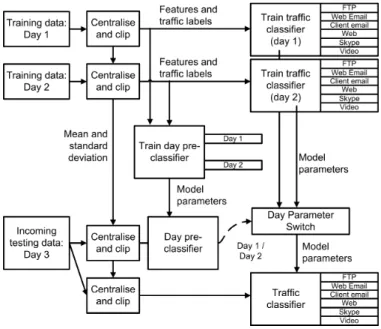
as classifiers cannot always be updated online all the time. It was also noted that some days are more closely matched than others. Therefore, we propose here a pre-classifier stage to work out which training set best matches the test conditions. The binary version of the TRAP-VQ algorithm was used to see if appropriate training data could be selected. The classes of the input data were overwritten with the day number and used as training sets.
Two situations were analysed: firstly training on days 1 and 2 to test on day 3 and secondly using days 1 to 3 to test on day 4. An overview of the system can be seen in Figure 6. The binary version of the TRAP-VQ algorithm was also used as the main traffic classification algorithm.Note for comparison purposes, the pre-classifier results were included in Figure 4, as algorithm number 12. Results are only plotted where multiple choices of training data sets are available (e.g., when testing against days 3 and 4).
Fig. 6. WLAN traffic classification system overview, incorporating pre-classifier
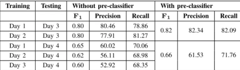
The pre-classifier analyses each feature vector and decides which training set should be used. In reality, all models are generated prior to deployment and the pre-classifier simply switches the output to the appropriate model. As can be seen from the results in Table VII, the pre-classifier improves the F1 when testing against days 3 and 4. Figure 4 also shows how the pre-classifier improves performance over many of the other classification algorithms tested. Putting features from multiple days together into a single data set for training was also investigated; however, this caused the resulting F1 to decrease.
When this traffic classification system is in use, it is envisaged that as further training sets became available they can be loaded into the system and the pre-classifier can make a decision as to which set best matches the current testing conditions. In this manner, the system optimises itself as data becomes available. This means that system training can be carried out off-line, and once trained a new pre-classifier entry
and associated tree for traffic classification becomes available to the system.
TABLE VII
RESULTS USING A PRE-CLASSIFIER
Training Testing Without pre-classifier With pre-classifier
F1 Precision Recall F1 Precision Recall Day 1 Day 3 0.80 80.46 78.86 0.82 82.34 82.09 Day 2 Day 3 0.80 77.91 81.27 Day 1 Day 4 0.65 60.02 70.06 0.66 61.53 71.76 Day 2 Day 4 0.62 56.11 68.98 Day 3 Day 4 0.60 52.92 68.35 VIII. CONCLUSION
The ability to classify network traffic is important for many routine network management applications. In a related area, businesses are making use of passive WLAN monitoring devices to improve both network performance and security. This paper has brought together the areas of network traf-fic classitraf-fication and passive WLAN monitoring. A cheap (< $15) WLAN dongle was utilised to monitor a network and perform traffic classification. It is desirable to cheaply upgrade a firm’s existing assets, for example, by attaching a WLAN dongle to desktop machines to be used when local user related processing is minimal. This reduces the burden on existing network hardware that can be costly to upgrade. It is undesirable, from a security perspective, to pass network keys to all passive monitoring nodes. Hence, traffic classification on wireless traffic can be more challenging than wired traffic, as much of the information from higher layers of the stack (which would potentially be available even on an encrypted wired network) has been encrypted by the wireless bearer.
A WLAN data set was created that spans multiple days and includes both multiple traffic types and applications. Analysis was performed on 63 features based on statistics of packet length and IAT. It was shown that features in the uplink and downlink directions were substantially different; hence, directionality (uplink/downlink) was incorporated into the feature vectors. Six ML algorithms were tested, one of which (the GMM-UBM) has not been used to classify wired or wireless traffic before. The GMM-UBM generally had increased performance over the standard GMM.
Additionally, an ML algorithm referred to as TRAP-VQ was proposed by the authors to be more suited to WLAN traffic classification, in terms of its computational complexity and prior knowledge requirements. When training and testing on the same day the TRAP-VQ algorithm gave the highest F1. It was noted that when training and testing using data from different days the F1 decreased. In order to compensate for this, a TRAP-VQ pre-classifier stage was added to find training data that most adequately matched the testing conditions and improved performance.
REFERENCES
[1] T. Karagiannis, A. Broido, N. Brownlee, K. Claffy, and M. Faloutsos, “Is P2P dying or just hiding? [P2P traffic measurement],” in Global Telecommunications Conference, 2004. GLOBECOM ’04. IEEE, vol. 3, pp. 1532–1538 Vol.3, Nov 2004.
[2] M. Roughan, S. Sen, O. Spatscheck, and N. Duffield, “Class-of-service mapping for qos: A statistical signature-based approach to ip traffic classification,” inProceedings of the 4th ACM SIGCOMM Conference on Internet Measurement, IMC ’04, (New York, NY, USA), pp. 135– 148, ACM, 2004.
[3] A. W. Moore and D. Zuev, “Internet traffic classification using bayesian analysis techniques,” in Proceedings of the 2005 ACM SIGMETRICS International Conference on Measurement and Modeling of Computer Systems, SIGMETRICS ’05, (New York, NY, USA), pp. 50–60, ACM, 2005.
[4] T. Karagiannis, K. Papagiannaki, and M. Faloutsos, “Blinc: Multilevel traffic classification in the dark,” in Proceedings of the 2005 Confer-ence on Applications, Technologies, Architectures, and Protocols for Computer Communications, SIGCOMM ’05, (New York, NY, USA), pp. 229–240, ACM, 2005.
[5] “SSL encrypted traffic over the WAN increasing.” http://www. net-security.org/secworld.php?id=4852Webpage. Accessed May 2013. [6] “Air patrol - location is everything.” http://airpatrolcorp.com/. Accessed
February 2015.
[7] “Airmagnet wifi analyser pro.” http://www.flukenetworks.com/enterprise-network/wireless-network/AirMagnet-WiFi-Analyzer, Accessed February 2015.
[8] M. Research, “Dair: A framework for managing enterprise wireless networks using desktop infrastructure.” http://research.microsoft.com/en-us/um/people/alecw/hotnets-2005.pdf, 2005.
[9] W. Lu, M. Tavallaee, and A. Ghorbani, “Hybrid traffic classification approach based on decision tree,” inGlobal Telecommunications Con-ference, 2009. GLOBECOM 2009. IEEE, pp. 1–6, Nov 2009. [10] R. Braden, D. Clark, and S. Shenker, “Integrated services in the internet
architecture: an overview,”RFC 1633, May 2004.
[11] S. Blake, D. Black, M. Carlson, E. Davies, D. Wang, and W. Weiss, “An architecture for differentiated services,”RFC 2475, IETF, 1998. [12] T. T. T. Nguyen, G. Armitage, P. Branch, and S. Zander, “Timely
and continuous machine-learning-based classification for interactive ip traffic,” Networking, IEEE/ACM Transactions on, vol. 20, pp. 1880– 1894, Dec 2012.
[13] A. Mcgregor, M. Hall, P. Lorier, and J. Brunskill, “Flow clustering using machine learning techniques,” inIn PAM, pp. 205–214, 2004. [14] M. Roughan, S. Sen, O. Spatscheck, and N. Duffield, “Class-of-service
mapping for qos: A statistical signature-based approach to ip traffic classification,” inProceedings of the 4th ACM SIGCOMM Conference on Internet Measurement, IMC ’04, (New York, NY, USA), pp. 135– 148, ACM, 2004.
[15] S. Zander, T. Nguyen, and G. Armitage, “Automated traffic classifi-cation and appliclassifi-cation identificlassifi-cation using machine learning,” inLocal Computer Networks, 2005. 30th Anniversary. The IEEE Conference on, pp. 250–257, Nov 2005.
[16] J. Erman, M. Arlitt, and A. Mahanti, “Traffic classification using clustering algorithms,” inProceedings of the 2006 SIGCOMM Workshop on Mining Network Data, MineNet ’06, (New York, NY, USA), pp. 281– 286, ACM, 2006.
[17] G. Xie, M. Iliofotou, R. Keralapura, M. Faloutsos, and A. Nucci, “Subflow: Towards practical flow-level traffic classification,” in IEEE INFOCOM (mini-conference), (Orlando, FL, USA), March 2012. [18] N. Jing, M. Yang, S. Cheng, Q. Dong, and H. Xiong, “An efficient
svm-based method for multi-class network traffic classification,” in Performance Computing and Communications Conference (IPCCC), 2011 IEEE 30th International, pp. 1–8, Nov 2011.
[19] M. Crotti, F. Gringoli, and L. Salgarelli, “Impact of asymmetric rout-ing on statistical traffic classification,” in Global Telecommunications Conference, 2009. GLOBECOM 2009. IEEE, pp. 1–8, Nov 2009. [20] P. Haffner, S. Sen, O. Spatscheck, and D. Wang, “Acas: Automated
construction of application signatures,” in In SIGCOMM05 MineNet Workshop, 2005.
[21] A. W. Moore and D. Zuev, “Internet traffic classification using bayesian analysis techniques,”SIGMETRICS Perform. Eval. Rev., vol. 33, pp. 50– 60, June 2005.
[22] N. Williams, S. Zander, and G. Armitage, “A preliminary performance comparison of five machine learning algorithms for practical ip traffic flow classification,”SIGCOMM Comput. Commun. Rev., vol. 36, pp. 5– 16, Oct. 2006.
[23] T. Auld, A. Moore, and S. Gull, “Bayesian neural networks for internet traffic classification,”Neural Networks, IEEE Transactions on, vol. 18, pp. 223–239, Jan 2007.
[24] P. Lin, Z. Lei, L. Chen, J. Yang, and F. Liu, “Decision tree network traffic classifier via adaptive hierarchical clustering for imperfect training
dataset,” inWireless Communications, Networking and Mobile Comput-ing, 2009. WiCom ’09. 5th International Conference on, pp. 1–6, Sept 2009.
[25] D. Qin, J. Yang, J. Wang, and B. Zhang, “Ip traffic classification based on machine learning,” inCommunication Technology (ICCT), 2011 IEEE 13th International Conference on, pp. 882–886, Sept 2011.
[26] J. Park, H.-R. Tyan, and C.-C. Kuo, “Internet traffic classification for scalable qos provision,” inMultimedia and Expo, 2006 IEEE Interna-tional Conference on, pp. 1221–1224, July 2006.
[27] S. Ubik and P. Zejdl, “Evaluating application-layer classification using a machine learning technique over different high speed networks,” in Sys-tems and Networks Communications (ICSNC), 2010 Fifth International Conference on, pp. 387–391, Aug 2010.
[28] B. Hullar, S. Laki, and A. Gyorgy, “Early identification of peer-to-peer traffic,” inCommunications (ICC), 2011 IEEE International Conference on, pp. 1–6, June 2011.
[29] L. Peng, H. Zhang, B. Yang, Y. Chen, M. Qassrawi, and G. Lu, “Traffic identification using flexible neural trees,” inQuality of Service (IWQoS), 2010 18th International Workshop on, pp. 1–5, June 2010.
[30] K. Singh and S. Agrawal, “Comparative analysis of five machine learning algorithms for ip traffic classification,” inEmerging Trends in Networks and Computer Communications (ETNCC), 2011 International Conference on, pp. 33–38, April 2011.
[31] F. Dehghani, N. Movahhedinia, M. Khayyambashi, and S. Kianian, “Real-time traffic classification based on statistical and payload content features,” in Intelligent Systems and Applications (ISA), 2010 2nd International Workshop on, pp. 1–4, May 2010.
[32] R. Alshammari and A. N. Zincir-Heywood, “An investigation on the identification of voip traffic: Case study on gtalk and skype.,” inCNSM, pp. 310–313, IEEE, 2010.
[33] C. Bacquet, A. Zincir-Heywood, and M. Heywood, “Genetic optimiza-tion and hierarchical clustering applied to encrypted traffic identifica-tion,” in Computational Intelligence in Cyber Security (CICS), 2011 IEEE Symposium on, pp. 194–201, April 2011.
[34] D. Bonfiglio, M. Mellia, M. Meo, D. Rossi, and P. Tofanelli, “Revealing skype traffic: When randomness plays with you,”SIGCOMM Comput. Commun. Rev., vol. 37, pp. 37–48, Aug. 2007.
[35] T. En-Najjary, G. Urvoy-Keller, M. Pietrzyk, and J.-L. Costeux, “Application-based feature selection for internet traffic classification,” inTeletraffic Congress (ITC), 2010 22nd International, pp. 1–8, Sept 2010.
[36] M. Ichino, H. Maeda, T. Yamashita, K. Hoshi, N. Komatsu, K. Takeshita, M. Tsujino, M. Iwashita, and H. Yoshino, “Internet traffic classification using score level fusion of multiple classifier,” inComputer and Infor-mation Science (ICIS), 2010 IEEE/ACIS 9th International Conference on, pp. 105–110, Aug 2010.
[37] F. Zhang, W. He, and X. Liu, “Defending against traffic analysis in wireless networks through traffic reshaping,” inDistributed Computing Systems (ICDCS), 2011 31st International Conference on, pp. 593–602, June 2011.
[38] T. Nguyen and G. Armitage, “A survey of techniques for internet traffic classification using machine learning,”Communications Surveys Tutorials, IEEE, vol. 10, pp. 56–76, Fourth 2008.
[39] “Wireshark.” http://www.wireshark.org/. Accessed May 2013. [40] “H.264/avc software coordination.” http://iphome.hhi.de/suehring/tml/. [41] “Filezilla.” https://filezilla-project.org/. Accessed May 2013. [42] “Morzilla thunderbird.” https://www.mozilla.org/en-GB/thunderbird/. [43] S. A. Dudani, “The distance-weighted k-nearest-neighbor rule,”Systems,
Man and Cybernetics, IEEE Transactions on, vol. SMC-6, pp. 325–327, April 1976.
[44] D. A. Reynolds, T. F. Quatieri, and R. B. Dunn, “Speaker verification using adapted gaussian mixture models,” inDigital Signal Processing, p. 2000, 2000.
[45] L. Breiman, H. Friedman, R. A. Olshen, and C. J. Stone,Classification and Regression Trees. Wadsworth, 1984.
[46] D. POWERS, “Evaluation: From precision, recall and f-measure to roc, informedness, markedness & correlation,”Journal of Machine Learning Technologies, vol. 2, no. 1, pp. 37–63, 2011.
Dr. Joe Kornycky Received his BEng (Hons.) degree in electronic engi-neering from the University of Surrey, UK., in 2006. A Nokia scholarship was obtained throughout his undergraduate degree. He received a Ph.D. in Digital Signal Processing (DSP) from the Center for Communication Systems
Research (CCSR), University of Surrey, Guildford, U.K., 2010. His Ph.D. thesis was entitled acoustic source separation for static and moving targets. He joined the Defence Science and Technology Laboratory (Dstl) in 2009. Since then the focus of his work has moved from DSP applied to audio and acoustics, to DSP applied to Radio Frequency (RF) communications signals and systems. He obtained the Graham Mathieson award in 2013 for outstanding service while working at Dstl. His main research interests include DSP, audio processing, Telecommunications and RF, array signal processing, statistical processing, unsupervised adaptive beamforming, artificial intelligence and machine learning.
Dr. Omar Abdul-HameedOmar Abdul-Hameed re-ceived his BEng degree in Electronic and Electrical Engineering with a First Class Honours from the University of Surrey, UK in 2003. He then joined the I-Lab, Multimedia Communications Research at the University of Surrey where he obtained his Ph.D. degree in 2009. From 2007 to 2014, he has been actively involved and working in several EU-funded FP6 and FP7 collaborative research projects as a Research Fellow. He then joined the Institute for Digital Technologies (IDT) at Loughborough Uni-versity London in October 2014 as a Research Associate. His main research interests include radio resource management in mobile broadband networks, end-to-end QoS across heterogeneous access networks, experimental test-bed design and implementation with IP-based multimedia applications, and conducting research in technologies for 5G communications. He has several publications in international journals and conferences as well as several book chapters.
Prof. Ahmet Kondozreceived his PhD in 1987 from the University of Surrey where he was a research fellow in the communication systems research group until 1988. He became a lecturer in 1988, reader in 1995, and in 1996 he was promoted to profes-sor in multimedia communication systems. He was the founding head of I-LAB, a multi-disciplinary multimedia communication systems research lab at the University of Surrey. Since January 2014, Prof. Kondoz has been appointed as the founding Di-rector of the Institute for Digital Technologies, at Loughborough University London, a post graduate teaching, research and enterprise institute. He is also Associate Dean for Research for Loughborough University London. His research interests are in the areas of digital signal processing and coding, fixed and mobile multimedia communication systems, 3D immersive media applications for the future Internet systems, smart systems such as autonomous vehicles and assistive technologies, big data analytics and visualisation and related cyber security systems. He has over 400 publications, including six books, several book chapters, and seven international patents, and graduated more than 75 PhD students. He has been a consultant for major wireless media industries and has been acting as an advisor for various international governmental departments, research councils and patent attorneys. He is a director of MulSys Ltd., a university spin-off company marketing the worlds first secure GSM communication system through the mobile voice channel.
Professor Kondoz has been involved with several European Commission FP6 & FP7 research and development projects, such as NEWCOM, e-SENSE, SUIT, VISNET, MUSCADE etc. involving leading universities, research institutes and industrial organisations across Europe. He coordinated FP6 VISNET II NoE, FP7 DIOMEDES STREP and ROMEO IP projects, involving many leading organisations across Europe which deals with the hybrid delivery of high quality 3D immersive media to remote collaborating users including those with mobile terminals. He co-chaired the European networked media advisory task force, and contributed to the Future Media and 3D Internet activities to support the European Commission in the FP7.
Dr. Brian C. BarberBrian C. Barber received the BSc (honours) degree in physics from the University of Bristol U.K. in 1969 and the MSc degree in mathematics from the University of London UK in 1979. He joined the Royal Aircraft Establishment (RAE) at Farnborough UK in 1969 and in the 1970’s he worked on signal processing applied to synthetic aperture radar systems. Since then, he has specialised in various aspects of signal processing at RAE, the Defence Research Agency, and the Defence Science and Technology Laboratory (Dstl). He is currently a Fellow at Dstl and a visiting Professor at Strathclyde University UK.