Multi-criteria optimisation for complex
learning prediction systems
BASSMA
AL-JUBOURI
A thesis submitted in partial fulfilment of the requirements of
Bournemouth University for the degree of
Doctor of Philosophy
First Supervisor:
Prof. Bogdan Gabrys
Second Supervisor:
Dr. Emili Balaguer-Ballester
This copy of the thesis has been supplied on condition that anyone who consults it is understood to recognise that its copyright rests with its author and due acknowledgement must always be made of the use of any material contained in, or derived from, this thesis.
Abstract
This work presents a framework for the inclusion of multiple criteria in the design pro-cess of supervised learning algorithms; as well as studies the sophisticated interactions among them. The criteria included and tested experimentally in this thesis are: accuracy, model complexity, algorithmic complexity, diversity and robustness.
The present thesis addresses important challenges related to considering multiple criteria such as: 1) defining suitable measures for the included criteria, 2) determining effective approaches to optimise the system performance using multiple objectives, 3) finding ef-fective alternative approaches to include such criteria indirectly in the design stages when defining accurate measures is infeasible, and finally 4) analysing the possible interactions among the criteria as well as identifying the main factors/decision points that modulate them.
This work introduces a novel Multi-Components, Multi-Layer Predictive System (MCMLPS). This system incorporates mechanisms designed to control the diversity, model complexity and robustness.
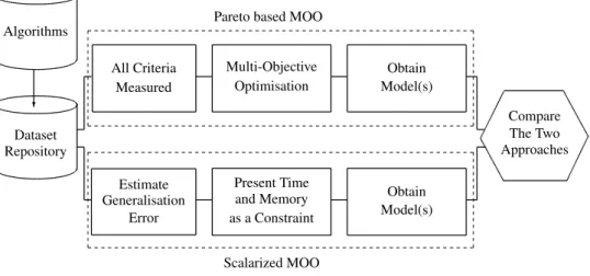
In the first stage of this thesis, the accuracy, model and algorithmic complexities of the base components for the proposed system have been optimised empirically using two multi-objective optimisation approaches. The first approach consists of a scalarized multi-objective optimisation, where the models are generated from optimising a single cost function that combines the three criteria. The second approach uses a Pareto-based multi objective optimisation which establishes a trade-off among the three criteria to gen-erate a set of selectively balanced models.
These first results showed that models generated from Pareto-based multi objective op-timisation approach are both more accurate and more diverse than the models generated from scalarized multi-objective optimisation approach. However, the Pareto-based ap-proach is hindered by the high algorithmic complexity required to find the best model and the infeasibility of defining universal measures for some of the above-mentioned cri-teria. Thus, in later stages of this work these criteria are either presented as constraints or included indirectly in generating the base components for the MCMLPS.
In a subsequent stage of this study, the diversity among the base components of the pro-posed MCMLPS system is encouraged by training them on local regions in the data, were the locality is determined using the similarity of the data features. Each local re-gion contains either disjoint subsets of the data and/or subsets of the features. A range of similarity metrics such as pairwise squared correlation and conditional mutual
informa-tion of the features are used. Interestingly, the squared correlainforma-tion method can be applied in supervised as well as unsupervised learning as it does not consider the output class when splitting the data. Meanwhile, the conditional mutual information method can be applied only in supervised learning as it uses the output class in splitting the data. The full MCMLPS architecture is then analysed and its performance is compared to three well-known ensemble methods.
Next, the effect of weighing the components of the MCMLPS and combining them is examined using six fusion methods. The results showed that, including the similarity metric used to divide the data into local regions in weighing the system components, of-ten results in the best accuracy compared to the other fusion methods.
In the final phase of this study, the robustness of the proposed system in noisy environ-ments is tested and compared to other ensemble methods. The system showed a compara-ble accuracy to the best performing ensemcompara-ble and it often has a more robust performance than other ensembles in highly noisy environments.
To conclude, the present thesis proposes a multi-component, multi-layer system which simultaneously incorporates multiple criteria in its design cycle. The results of this the-sis suggest that the locality in learning and high diversity among the components of the proposed system can be particularly beneficial in designing ensemble learning methods for highly noisy data sets.
Contents
Copyright statement . . . i
Abstract . . . iii
Table of contents . . . v
List of figures . . . ix
List of tables . . . xiii
Nomenclature xviii List of Abbreviations . . . xxi
Acknowledgements . . . xxiii
Declaration . . . xxv
Dedication . . . xxvii
1 Introduction 1 1.1 Background . . . 3
1.2 Project Description and Goals . . . 4
1.3 Contributions . . . 6
1.4 Thesis Organization . . . 7
1.5 Publications resulted from this work . . . 8
2 Predictive Systems: Representation, Evaluation and Optimisation 9 2.1 Introduction . . . 9
2.2 Predictive Systems Architectures . . . 12
2.3 Predictive Systems Evaluation . . . 19
2.3.1 Accuracy . . . 19
2.3.2 Complexity . . . 23
2.3.2.1 Algorithmic Complexity Measures . . . 24
2.3.2.2 Model Complexity Measures . . . 26
2.3.3 Robustness . . . 28
2.3.3.1 Stability . . . 30
2.3.4 Adaptation . . . 30
2.3.5 Transparency . . . 31
2.4 Predictive System Optimisation . . . 32
2.4.1 Single Objective Optimisation . . . 32
2.4.2 Scalarized Multi-Objective Optimisation . . . 33
2.4.3 Multi-Objective Optimisation . . . 34
2.4.4 Hierarchical Optimisation . . . 35
2.4.5 Comparing Optimization Approaches . . . 36
2.5 Summary . . . 37
3 Design Cycle of Multi-Component, Multi-Layer Predictive System and Base Models Generation 39 3.1 Introduction . . . 39
3.2 General Design Cycle of MCMLPS . . . 40
3.2.1 Pre-Processing . . . 41
3.2.2 Model generation . . . 43
3.2.3 Model evaluation . . . 43
3.2.4 Model optimisation . . . 45
3.2.5 Post-processing . . . 45
3.3 Comparing Multi-criteria Predictive Models generated from Scalarized MOO and Pareto-based MOO . . . 46
3.3.1 Methodology . . . 48
3.3.2 Results . . . 50
3.3.3 Increasing the Population Size and the Maximum Number of Generation in the Pareto based MOO . . . 51
3.3.4 Limitations of the optimisation approaches . . . 52
3.4 Summary . . . 60
4 Diversity in Multi-component, Multi-layer Predictive System 61 4.1 Introduction . . . 61
4.2 Multi-Component, Multi-Layer Predictive Systems . . . 62
4.3 Diversity Methods Categorization . . . 64
4.4.1 Feature extraction and feature selection . . . 66
4.5 Locally weighted predictive systems . . . 67
4.6 Designing MCMLPS: Methodology . . . 69
4.6.1 Correlation based LRs . . . 71
4.6.1.1 Results . . . 73
4.6.1.2 Internal Accuracies and Benchmark Comparison . . . . 74
4.6.1.3 Changing the type of the base predictors . . . 77
4.6.1.4 Disagreements among the base predictors . . . 78
4.6.2 Conditional mutual information based LRs . . . 80
4.6.2.1 Results . . . 82
4.6.2.2 Internal accuracy and benchmark comparison . . . 82
4.6.2.3 Disagreements among the base predictors . . . 84
4.6.2.4 Variation of the conditional mutual information . . . . 86
4.6.2.5 Ignoring the inner correlation with respect to the class . 86 4.6.2.6 Using Cross Validation instead of DPS . . . 88
4.6.2.7 Changing the ratio of the features used in the LRs . . . 90
4.7 Summary . . . 91
5 Multi-Component, Multi-Layer Predictive System in Noisy Environments 93 5.1 Introduction . . . 93
5.2 The effect of noise on system prediction . . . 94
5.3 Balancing Robustness and Flexibility . . . 96
5.4 Testing the MCMLPS in noisy environments . . . 97
5.4.1 Results . . . 98
5.4.2 Discussion . . . 107
5.5 The Effect of Changing the Fusion Methods on MCMLPS Performance . 108 5.5.1 Single local region . . . 109
5.5.2 Best Model . . . 111
5.5.3 Majority vote . . . 114
5.5.4 Weighted majority vote . . . 116
5.5.5 The relative loss of accuracy for the six fusion methods . . . 123
5.5.6 Discussion . . . 124
5.6 Summary . . . 126
6.1 Thesis summary . . . 129 6.2 Main contributions . . . 131 6.3 Future work . . . 133
A Data Sets Descriptions 135
B The accuracy and RLA for the MCMLPS fusion methods 139
B.1 The accuracy of the six fusion methods . . . 139 B.1.1 Accuracy for the six fusion methods in the correlation based
MCMLPS . . . 139 B.1.2 The accuracy for the six fusion methods in the MI based MCMLPS143 B.2 The relative loss of accuracy in the six fusion methods . . . 147
B.2.1 The RLA for the six fusion methods in the correlation based MCMLPS . . . 147 B.2.2 The RLA for the six fusion methods in the MI based MCMLPS . 151
List of Figures
2.1 The decomposition of the learning process (based on Domingos (2012)) . 12 2.2 A Simple illustration for a single predictor consisting of a pre-processing
unit, a prediction function and a post-processing unit . . . 13
2.3 The bias-variance dilemma. Adopted from (Fortmann-Roe (2012)) . . . . 14
2.4 An illustration for a homogeneous ensemble consisting of multiple pre-dictors of the same type . . . 16
2.5 An illustration for a heterogeneous ensemble consisting of multiple pre-dictors of different types . . . 17
2.6 An illustration for a pool of competing predictors/ensembles . . . 18
2.7 The ROC curve for classifying the Virginica class in the Fisher iris data set using logistic regression . . . 22
2.8 A data set fitted with three functions of increasing complexity. Adopted from Gunn (2012). . . 24
2.9 Optimising a single criterion . . . 33
2.10 Optimising multiple criteria using scalarized MOO . . . 33
2.11 Optimising multiple criteria using hierarchical optimisation . . . 35
3.1 Generalized design Cycle of MCMLPS . . . 40
3.2 The two approaches for evaluating and optimising predictive models. . . . 46
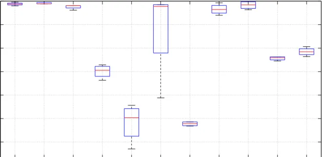
3.3 a) Comparing the predictive model accuracy (MSE), model complexity and execution time of the models generated using the scalarized MOO approach and the Pareto-based MOO approach (with 10 population size and a maximum number of generation of 10). . . 54
3.3 b) Comparing the predictive model accuracy (MSE), model complexity and execution time of the models generated using the scalarized MOO approach and the Pareto-based MOO approach (with 10 population size and a maximum number of generation of 10). . . 55 3.3 c) Comparing the predictive model accuracy (MSE), model complexity
and execution time of the models generated using the scalarized MOO approach and the Pareto-based MOO approach (with 10 population size and a maximum number of generation of 10). . . 56 3.4 a) Comparing the predictive model accuracy (MSE), model complexity
and execution time of the models generated using the scalarized MOO approach and the Pareto-based MOO approach (with 100 population size and a maximum number of generation of 100). . . 57 3.4 b) Comparing the predictive model accuracy (MSE), model complexity
and execution time of the models generated using the scalarized MOO approach and the Pareto-based MOO approach (with 100 population size and a maximum number of generation of 100). . . 58 3.4 c) Comparing the predictive model accuracy (MSE), model complexity
and execution time of the models generated using the scalarized MOO approach and the Pareto-based MOO approach (with 100 population size and a maximum number of generation of 100). . . 59 4.1 General structure for the multi-component, multi-layer predictive system. 63 4.2 Data preparation and model generation. . . 70 4.3 Training accuracies of the local regions models for the correlation based
MCMLPS when applied to Gaussian 8D data set. . . 75 4.4 comparing the disagreements among the classifier/LR of both RF and
MCMLPS, the base predictors used are: NN and CART DTs., where
1 =LR DT,2 =LR NN,3 =RF DT and4 =RF NN . . . 79 4.5 Training accuracies of the local regions models for the MI based
MCMLPS when applied to Gaussian 8D data set. . . 83 4.6 Comparing the disagreements among the LRs of MI based MCMLPS
when CART DTs are used as the base predictors. . . 85 4.7 Comparing the disagreements among the LRs of MI based MCMLPS
4.8 Comparing the accuracy of the system when the data is split using CMI
and traditional feature selection , part I. . . 87
4.8 Comparing the accuracy of the system when the data is split using CMI and traditional feature selection , part II . . . 88
4.9 Comparing the accuracy of the system when the data is split using CV and DPS, part I. . . 89
4.9 Comparing the accuracy of the system when the data is split using CV and DPS, part II . . . 90
5.1 Comparing the accuracy of the five benchmark algorithms in noisy envi-ronments for the Gaussian 8D data set. . . 99
5.2 Comparing the accuracy of the five benchmark algorithms in noisy envi-ronments for the German credit card data set. . . 99
5.3 Comparing the accuracy of the five benchmark algorithms in noisy envi-ronments for the ionosphere data set. . . 99
5.4 Comparing the accuracy of the five benchmark algorithms in noisy envi-ronments for the spam base data set. . . 100
5.5 Comparing the accuracy of the five benchmark algorithms in noisy envi-ronments for the Pima Indian diabetes data set. . . 100
5.6 Comparing the accuracy of the five benchmark algorithms in noisy envi-ronments for the WBC data set. . . 100
5.7 Comparing the accuracy of the five benchmark algorithms in noisy envi-ronments for the heart data set. . . 101
5.8 Comparing the accuracy of the five benchmark algorithms in noisy envi-ronments for the sonar data set. . . 101
5.9 Comparing the accuracy of the five benchmark algorithms in noisy envi-ronments for the chess data set. . . 101
5.10 Comparing the accuracy of the five benchmark algorithms in noisy envi-ronments for the vehicle data set. . . 102
5.11 Comparing the accuracy of the five benchmark algorithms in noisy envi-ronments for the waveform data set. . . 102
5.12 An illustration for the MCMLPS with single LR fusion method . . . 110
5.13 An illustration for the MCMLPS with best model fusion method . . . 113
5.15 An illustration for the MCMLPS with MV weighted by similarity in all layers . . . 118 5.16 An illustration for the MCMLPS with MV weighted by similarity and
normalized training accuracy in the first layer and the similarity in sub-sequent layers . . . 119 5.17 An illustration for the MCMLPS with MV weighted by similarity and
normalized training accuracy in the first layer and the similarity and av-erage training accuracy in subsequent layers . . . 120
List of Tables
2.1 Confusion matrix for binary classification problems . . . 20 2.2 Learning methods used to generate linear and quadratic predictive
Mod-els . . . 24 3.1 Data set details . . . 47 4.1 Comparing rotation forest, squared correlation and conditional MI
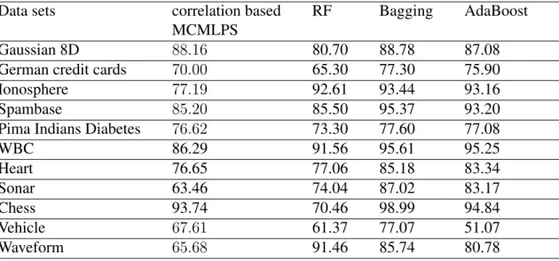
en-semble methods . . . 69 4.2 Weights calculation for the illustrative example. . . 71 4.3 Data sets details . . . 74 4.4 Comparing the test accuracies of the four ensemble methods when CART
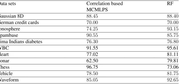
DTs are used as their base predictors. . . 77 4.5 Comparing the test accuracies of correlation based MCMLPS and RF
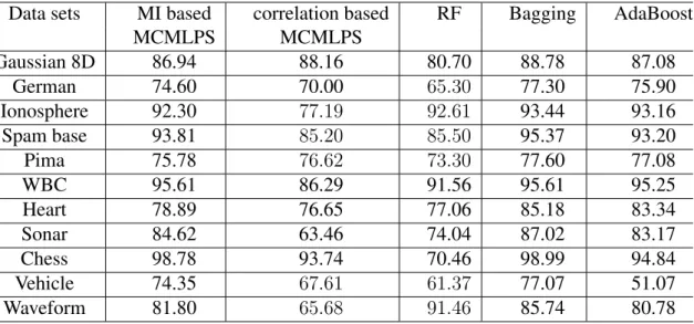
when feedforward NNs are used as their base predictors. . . 78 4.6 Comparing the test accuracies of the five ensemble methods when CART
DTs are used as their base predictors. . . 84 4.7 Comparing the test accuracies of MI based MCMLPS, correlation based
MCMLPS and RF when feedforward NNs are used as their base predictors. 85 5.1 The standard deviations of the accuracy for the five ensemble methods
when applied to data sets with five different noise ratios. . . 104 5.2 The relative loss in accuracy for the five ensemble methods when noise
is added to the training (TR) and testing (TS) data . . . 105 5.3 The standard deviations of the accuracy for single LR fusion method
when applied with correlation based and MI based MCMLPS. . . 112 5.4 The standard deviations of the accuracy for the best model fusion method
when applied with correlation based and MI based MCMLPS. . . 114
5.5 The standard deviations of the accuracy for the best model fusion method when applied with correlation based and MI based MCMLPS. . . 116 5.6 The standard deviations of the accuracy for the WMV fusion methods
when applied with correlation based and MI based MCMLPS. . . 121 5.7 The accuracy of the fusion methods for the correlation based MCMLPS
when applied to the Gaussian 8 dimensions data set. . . 121 5.8 The accuracy of the fusion methods for the MI based MCMLPS when
applied to the ionosphere data set. . . 121 5.9 The accuracy of the fusion methods for the correlation based MCMLPS
when applied to the ionosphere data set. . . 122 5.10 The accuracy of the fusion methods for the MI based MCMLPS when
applied to the Pima data set. . . 122 5.11 The accuracy of the fusion methods for the correlation based MCMLPS
when applied to the sonar data set. . . 122 5.12 The accuracy of the fusion methods for the MI based MCMLPS when
applied to the vehicle data set. . . 123 5.13 The accuracy of the fusion methods for the correlation based MCMLPS
when applied to the heart data set. . . 123 5.14 The accuracy of the fusion methods for the MI based MCMLPS when
applied to the German data set. . . 123 5.15 The count of the lowest RLA values for the six fusion methods . . . 124 B.1 The accuracy of the fusion methods for the correlation based MCMLPS
when applied to the Gaussian 8 dimensions data set. . . 140 B.2 The accuracy of the fusion methods for the correlation based MCMLPS
when applied to the German credit card data set. . . 140 B.3 The accuracy of the fusion methods for the correlation based MCMLPS
when applied to the ionosphere data set. . . 140 B.4 The accuracy of the fusion methods for the correlation based MCMLPS
when applied to the spam base data set. . . 141 B.5 The accuracy of the fusion methods for the correlation based MCMLPS
when applied to the Pima data set. . . 141 B.6 The accuracy of the fusion methods for the correlation based MCMLPS
B.7 The accuracy of the fusion methods for the correlation based MCMLPS when applied to the heart data set. . . 142 B.8 The accuracy of the fusion methods for the correlation based MCMLPS
when applied to the sonar data set. . . 142 B.9 The accuracy of the fusion methods for the correlation based MCMLPS
when applied to the chess data set. . . 142 B.10 The accuracy of the fusion methods for the correlation based MCMLPS
when applied to the Vehicle data set. . . 143 B.11 The accuracy of the fusion methods for the correlation based MCMLPS
when applied to the Waveform data set. . . 143 B.12 The accuracy of the fusion methods for the MI based MCMLPS when
applied to the Gaussian 8 dimensional data set. . . 143 B.13 The accuracy of the fusion methods for the MI based MCMLPS when
applied to the German data set. . . 144 B.14 The accuracy of the fusion methods for the MI based MCMLPS when
applied to the ionosphere data set. . . 144 B.15 The accuracy of the fusion methods for the MI based MCMLPS when
applied to the spam base data set. . . 144 B.16 The accuracy of the fusion methods for the MI based MCMLPS when
applied to the Pima data set. . . 145 B.17 The accuracy of the fusion methods for the MI based MCMLPS when
applied to the WBC data set. . . 145 B.18 The accuracy of the fusion methods for the MI based MCMLPS when
applied to the heart data set. . . 145 B.19 The accuracy of the fusion methods for the MI based MCMLPS when
applied to the sonar data set. . . 146 B.20 The accuracy of the fusion methods for the MI based MCMLPS when
applied to the chess data set. . . 146 B.21 The accuracy of the fusion methods for the MI based MCMLPS when
applied to the vehicle data set. . . 146 B.22 The accuracy of the fusion methods for the MI based MCMLPS when
applied to the waveform data set. . . 147 B.23 The RLA of the fusion methods for the correlation based MCMLPS when
B.24 The RLA of the fusion methods for the correlation based MCMLPS when applied to the German credit card data set. . . 148 B.25 The RLA of the fusion methods for the correlation based MCMLPS when
applied to the ionosphere data set. . . 148 B.26 The RLA of the fusion methods for the correlation based MCMLPS when
applied to the spam base data set. . . 148 B.27 The RLA of the fusion methods for the correlation based MCMLPS when
applied to the Pima data set. . . 149 B.28 The RLA of the fusion methods for the correlation based MCMLPS when
applied to the WBC data set. . . 149 B.29 The RLA of the fusion methods for the correlation based MCMLPS when
applied to the heart data set. . . 149 B.30 The RLA of the fusion methods for the correlation based MCMLPS when
applied to the sonar data set. . . 150 B.31 The RLA of the fusion methods for the correlation based MCMLPS when
applied to the chess data set. . . 150 B.32 The RLA of the fusion methods for the correlation based MCMLPS when
applied to the vehicle data set. . . 150 B.33 The RLA of the fusion methods for the correlation based MCMLPS when
applied to the waveform data set. . . 151 B.34 The RLA of the fusion methods for the MI based MCMLPS when applied
to the Gaussian 8 dimensional data set. . . 151 B.35 The RLA of the fusion methods for the MI based MCMLPS when applied
to the German data set. . . 151 B.36 The RLA of the fusion methods for the MI based MCMLPS when applied
to the ionosphere data set. . . 152 B.37 The RLA of the fusion methods for the MI based MCMLPS when applied
to the spam base data set. . . 152 B.38 The RLA of the fusion methods for the MI based MCMLPS when applied
to the Pima data set. . . 152 B.39 The RLA of the fusion methods for the MI based MCMLPS when applied
to the WBC data set. . . 153 B.40 The RLA of the fusion methods for the MI based MCMLPS when applied
B.41 The RLA of the fusion methods for the MI based MCMLPS when applied to the sonar data set. . . 153 B.42 The RLA of the fusion methods for the MI based MCMLPS when applied
to the chess data set. . . 154 B.43 The RLA of the fusion methods for the MI based MCMLPS when applied
to the vehicle data set. . . 154 B.44 The RLA of the fusion methods for the MI based MCMLPS when applied
Nomenclature
X Matrix x Vector x Scalar value X Domain D Dataset ˆ y Predicted value P(x) Probability function L(x) Loss function Cr(x) Criterion functionC(i, j) Cost function of prediction
Ω() Model complexity O() Big O notation
λ Regularization hyperparameter
W Weight matrix
I(x1, x2) Mutual information forx1andx2
RLAx%noise Relative Loss of Accuracy whenx%noise is added to the data
SVM Support Vector Machine
MCMLPS Multi-Components, Multi-Layer, Predictive System MOO Multi-Objective Optimization
MSE Mean Square Error DT Decision Trees NN Neural Network
NSGA Non-dominated Sorting Genetic Algorithm SOO Single Objective Optimisation
MLP Multi-Layer Perceptron PCA Principle Component Analysis LDA Linear Discriminate Analysis ICA Independent Component Analysis MI Mutual Information
LR Local Region
DPS Density Preserving Sampling ZCA Zero-phase Component Analysis CV Cross Validation
RF Rotation Forest
CMI Conditional Mutual Information WMV Weighted Majority Vote
RLA Relative Loss of Accuracy MV Majority Vote
First of all, I would like to express my gratitude to my supervisor Prof. Bogdan Gabrys for his guidance and support throughout this project. I am thankful for the time he spent discussing this work, and for his expert knowledge and invaluable feedback which helped me in developing and improving many aspects of this work.
My sincere thanks also go to my second supervisor Dr. Emili Balaguer-Ballester for his constant encouragement and support during my PhD. I am grateful for his constructive feedback and quick response which he had provided no matter how busy he was.
I am thankful to Dr. Marcin Budka and Prof. Hamid Bouchachia for their constructive feedback during the transfer. My thanks to Dr. Marcin for the comments and insights I had received from him during the writing of this thesis which helped me to improve the presentation of this work. Also, I am thankful to my former supervisor Dr. Jianbing Ma for his input in the early stages of this project. Others who contributed to this work are the anonymous reviewers whom their valuable feedback had helped me in improving and strengthening the work presented in this thesis.
Also, my thanks go to Naomi Bailey for her administrative advice and support during my PhD. Many thanks for my colleagues and friends in Bournemouth and back home for their help, support and encouragement.
I am deeply grateful to my family for their unconditional love and support, especially my parents who raised me with a love for science and support me in all my pursuits. Finally, I am thankful to the bless in my life, my sister, my colleague and my best friend Abeer. I am grateful for the long hours she spent discussing and reviewing the work presented in this thesis with me and for keeping me motivated at all time. Without her encouragement, love and support I would not be able to undertake this project.
The work contained in this thesis is the result of my own investigations and has not been accepted nor concurrently submitted in candidature for any other award.
To my parents
...
Mona and Khaldoon
Chapter 1
Introduction
Machine learning is considered as a relatively new field of research, however, collect-ing data and recognizcollect-ing distinctive patterns from it can be traced back at least to the 16th century, when Tycho Brahe recorded his astronomical observations (Dreyer (1890) and Swerdlow (1996)); which enabled Johannes Kepler to discover empirical laws of planetary motion (Small (1804) and Bishop (1995)). While pattern recognition has a long standing history, however, by the end of the first half of the 20th century all the main results in this field stem from statistics (Theodoridis and Koutroumbas (2006)). In the second half of the 20th century, machine learning had witnessed important de-velopments, starting from the work of Alan Turning in the 1950s (Turing (1950)) and continuing with the introduction of the first Neural Network (NN) machine by Marvin Minsky and Dean Edmonds (Russell and Norvig (2010)), and later with the development of the perceptron (Rosenblatt (1958)). During the AI winter in 1970s, the intensity of the research in this field slowed down (Cervier (1993)); but shortly thereafter, the exponential increase in computer power fostered again machine learning research (Theodoridis and Koutroumbas (2006)). Highly sophisticated algorithms such as deep learning or ensem-bles of learners that were infeasible in terms of their computational cost few decades ago are now commonly used in complex real-life settings (Deng and Yu (2014) and Zhang and Ma (2012)). Historically, machine learning systems have been designed to optimize the generalization ability of the system as the main criterion. The traditional aim of ma-chine learning is to design a system that can effectively learn regularities in the training data and then uses these identified regularities to perform tasks in the future, such as classifying the data into different classes with optimal accuracy (Bishop (1995)).
Nevertheless, as new learning systems which tackle different types of problems were in-troduced over the years, the need to include other criteria in the optimisation process of machine learning systems emerged (Jin (2006)). The concept of including more than one criterion in optimising the performance of machine learning systems has been the focus on a lively debate in the literature over the last two decades, for example:
• The inclusion of accuracy and model complexity has been revisited from the sta-tistical learning (Vapnik (2013)) and Bayesian angles (Moˇckus (1975)): the devel-oped systems should be accurate, yet their complexities should be bounded so that a complex system is not chosen for a problem that can be solved using a simpler system (Blumer et al. (1987)).
• The inclusion of accuracy and diversity: when multiple models are combined to produce the system, the diversity among them should be encouraged and monitored during the design stages (Cunningham and Carney (2000)). An ensemble with diverse models can have better performance due to the complementary behaviour of its components (Xue et al. (2006)).
• The inclusion of accuracy and robustness: the developed system should be able to tolerate certain variation in the data, yet it should be robust to outliers and noise (Xu et al. (2009)).
The above points shows that, previous approaches typically focus on pairs of criteria to optimise, in which one of them is the accuracy of the prediction (Jin (2006)). How-ever, the interaction among these criteria and the effect they have on each other is rarely discussed. The aim of this work is to design a novel framework which accounts for the multiple criteria in the optimization process for complex machine learning systems; and to study the effect of considering these criteria in the system performance in noisy datasets. Specifically, the criteria which are investigated in this work are the accuracy, model complexity, algorithmic complexity, diversity and robustness; which provide a rich description for the ensemble learning process from multiple angles. Furthermore, this work studies the feasibility of measuring these criteria, the advantages and draw-backs of including them in the optimization process, and most importantly the possible interactions among them.
1.1
Background
Predictive models that are built and trained with an overreliance on the prediction ac-curacy as the main optimisation criterion can result, as it is well-known, in some form of overfitting. Thus, heavily penalizing the complexity of the model whilst maintaining its accuracy has been a common strategy, for instance by the renowned Support Vector Machines (SVM) which optimise both accuracy and complexity through the use of struc-tural risk minimisation framework as a part of its training process (Cortes and Vapnik (1995),Vapnik (2013)).
However, model complexity is just one criterion among many other criteria that can affect the choice of predictive systems. In order to improve the performance of the prediction, ensemble learners are often used (Polikar (2006)). While these systems are substan-tially more sophisticated and have higher computational costs than a single predictor, combining different predictors can increase the accuracy of the overall system, provided enough diversity among the components of such systems i.e. their capacity to comple-ment each other is sufficiently observed. (e.g., Jacobs (1995), Meir (1995), Opitz and Shavlik (1996a) and Tumer and Ghosh (1996)). Though encouraging diversity among the base predictors of ensembles is widely acknowledged as an important issue in im-proving the ensemble performance (Bi (2012)), there has not been found a fundamental connection between the current diversity measures and the improvement of the prediction accuracy in general (Brown and Kuncheva (2010), Bi (2012) and Kuncheva and Whitaker (2003)).
In addition to improving the accuracy of the prediction, combining multiple classifiers has been linked to the ability of the system to perform well with noisy data (Ho et al. (1994)). Associating robustness to noise with Multi-Components, Multi-Layers Predic-tive System (MCMLPS) has been also traditionally linked to the diversity among the system base models: combining diverse models can improve the generalization ability of the system due to their complementary behaviour and allow the system to be less sub-jected to overfitting noisy data (Teng (1999) and S´aez et al. (2013)).
Unfortunately, defining effective measurements for the above- mentioned criteria is not always feasible in all machine learning methods. Thus, when measuring these criteria is infeasible, alternative mechanisms must be put in place to ensure that they are considered during the different stages of the predictive system design cycle, such as: a) using regu-larisation terms to penalize models with high complexity (Barron (1991)) and b) training
the ensemble base models on slightly different subsets of the data to encourage the diver-sity among them (Breiman (1996) and Rodriguez et al. (2006)).
Nevertheless, in cases when suitable measures for the multiple optimization criteria can be defined, Multi Objective Optimisation (MOO) approaches can be effectively used to maintain the desired trade-off among these criteria (Marler and Arora (2004) and Jin (2006)). There are a number of optimisation approaches for combining these criteria. One common approach is to use scalarization function which combines them into a single weighted sum and find the best possible model, such as: in neural networks regularisa-tion (Braga et al. (2006)) and in creating interpretable fuzzy rules (Jin (2000)). Another approach is to use Pareto-based MOO techniques to find a set of non-dominated solu-tions (models) that trade-off a set of conflicting criteria; such as: trading-off the accuracy versus the complexity of a radial basis function (Hatanaka et al. (2003)), trading-off false negative/false positive rates versus the number of support vectors to reduce the compu-tational complexity of an SVM (Suttorp and Igel (2006)) or developing a cost sensitive decision tree (Zhao (2007)) to cite a few.
In summary, considering multiple criteria in optimising complex predictive system entails unresolved challenges connected with how to find suitable measures of such criteria and how to include them in the design cycle of the predictive system. Also as was mentioned above, previous approaches typically focus on pairs of criteria to optimise in which one of them is the accuracy of the prediction (such as balancing accuracy and model complexity in (Yu et al. (2006)), or studying the effect of diversity with respect to the accuracy of the system (Cunningham and Carney (2000)). However, to the best of our knowledge studying the interaction among multiple criteria and the effect they have on each other have not previously been fully investigated; and will be the main focus of this thesis.
1.2
Project Description and Goals
This thesis emphasises the importance of including multiple criteria in the design process of predictive systems and studies the interaction among them. Furthermore, it compares the different optimisation approaches used to trade-off these criteria. The main goals of this work are:
• To identify the criteria used for evaluating the performance of a predictive system from multiple angles and to define effective measures for them when feasible.
• To develop strategies to include the selected criteria either directly in the optimisa-tion process or indirectly in the design process of the predictive system.
• To study the interactions among the included criteria and identify the main fac-tors/decision points in the MCMLPS that affect them.
This work examines the relations among the accuracy of the prediction, model complex-ity, algorithmic complexcomplex-ity, diversity and robustness. Furthermore, this project compares the efficiency of different optimisation techniques which can be used when multiple cri-teria are considered (Chapter 2 and 3). It examines the advantages and drawbacks in the cases when the criteria are combined in a single scalarized equation or when a trade-off among them is maintained (Chapter 3).
The initial experimental work considers the inclusion of the first three criteria (namely, the accuracy, model complexity and algorithmic complexity) in the optimisation process of the MCMLPS base components (Chapter 3). These experiments focus on different optimisation techniques used to include multiple criteria. Both Pareto-based MOO and scalarized MOO are used to generate the predictive models, and the performance of the resultant models is assessed and compared. The aims of these experiments are to examine the advantages and drawback of including multiple criteria and to compare the efficiency of the generated models using the two optimisation approaches.
Taking the above into consideration, a novel locally trained MCMLPS is introduced in Chapter 4. In this system, the diversity among the base models is maximized by training them on local disjoint sets of data and/or subsets of features. The data is divided into local regions using two approaches: an unsupervised approach which uses the feature similar-ity depending on their pairwise squared correlation and a supervised approach which is based on mutual information theory. This work is further developed to investigate the relation between the models diversity and their robustness to noise by introducing six fusion methods used to deliver the final prediction for the proposed MCMLPS (Chapter 5).
Finally, the interactions among the accuracy, diversity and robustness of this system is examined and the overall performance of the system is compared to a number of ensem-ble methods (Chapter 5). Our results indicated that the locality and high diversity among the components of the proposed system can provide a robust framework for designing complex systems in noisy environments.
1.3
Contributions
The following points summarise the main contributions in this work:
• A comprehensive theoretical study of predictive systems in terms of their archi-tectures, evaluation criteria and optimisation approaches. This study focuses on identifying measures for the principle criteria that affect the performance of ma-chine learning systems and whether universal measures can be defined for these criteria (Chapter 2).
• Conducting a new experiment in a representative, specifically designed case study which compares two MOO approaches and highlights the cost and benefits ob-tained from including multiple criteria in the optimisation of machine learning models in different classification settings (Chapter 3).
• A novel locally trained MCMLPS is next proposed (Chapter 4), where the locality of the system is introduced using two approaches:
– An unsupervised approach is used to split the data into disjoint subsets that are assigned to a set of local regions. The locality is determined using the pairwise squared correlation of the features. Then the base predictors of the MCMLPS are trained on these local regions. A particular benefit of MCMLPS is that, since it trained the local regions on disjoint subsets of the data, the diversity among its components is maximised.
– A supervised approach is used to split the data into local regions using the conditional mutual information of their features. In this approach the base models are trained on subsets of the features for all available data.
• An analysis of the robustness of the new MCMLPS in comparison with well-known ensemble methods; and its relation to the diversity of the proposed system in noisy environments (Chapter 5).
• The identification of the maindecision points (in the design and weighing of the MCMLPS) which influence the robustness, diversity and accuracy of the prediction (Chapter 5). These decision points are found to be:
– Data partitioning and model training.
– Weighing the prediction of the base models/ensembles.
1.4
Thesis Organization
Chapter 2 provides an overview of the learning process in predictive system. In Section 2.2 different architectures of predictive systems are explained, from simple single pre-dictor to complex multi-layer systems. Furthermore a survey of the predictive system evaluation criteria and their possible measurements is given in Section 2.3. Section 2.4 provides an overview of the optimisation approaches used to optimise single as well as multiple criteria of the predictive system.
In Chapter 3 the general methodology is discussed, starting with the design cycle of MCMLPS in Section 3.2. Next, Section 3.3 introduces a comparative case study specifi-cally designed to take into account the optimisation of predictive models using prediction accuracy, model complexity and algorithmic complexity. This new study compares the base models of MCMLPS that are generated from optimising the above mentioned cri-teria using scalarized multi-objective optimisation and Pareto-front multi-objective opti-misation. Furthermore, this section highlights the limitations associated with each of the two optimisation approaches.
Chapter 4 introduces a novel locally trained MCMLPS, where its base models are trained on disjoint subsets of the data and/or subsets of the features. The general architecture of the proposed system is given in Section 4.2. Section 4.3 compares the design cycle of MCMLPS with that of the rotation forest algorithm. Next, the methodology followed in designing the proposed system is given in Section 4.4 along with a detailed description of the metrics used to define the locality of the data, the experimental settings and the results.
Chapter 5 expands the work presented in Chapter 4 by testing the MCMLPS in noisy environments. The different types of noise and their effect on the performance of the system are explained in Section 5.2, while balancing the robustness and flexibility of machine learning models are the focus of Section 5.3. The first part of the experimental work in this Chapter is introduced in Section 5.4 where the proposed MCMLPS is tested in noisy environments and its performance is compared to other well-known ensemble methods. The second part of the experimental work, presented in Section 5.5, introduces six fusion methods to combine the base predictors of the MCMLPS and studies the effect of changing the fusion methods on the performance of the proposed system.
Finally, Chapter 6 concludes the thesis, summarising the main findings and contributions of this work and indicating directions for future research.
1.5
Publications resulted from this work
• Al-Jubouri, Bassma, and Bogdan Gabrys. ”Multicriteria approaches for predictive model generation: a comparative experimental study.” Computational Intelligence in Multi-Criteria Decision-Making (MCDM), 2014 IEEE Symposium on. IEEE, 2014.
• Al-Jubouri, Bassma, and Bogdan Gabrys. ”Local Learning for layer, Multi-component Predictive System.” Procedia Computer Science 96 (2016): 723-732. • Al-Jubouri, Bassma, and Gabrys, Bogdan. Diversity and Locality in
Multi-Component, Multi-Layer Predictive Systems: A Mutual Information Based Ap-proach In Advanced Data Mining and Applications: ADMA 2017, Singapore, November, 5-6, 2017. Springer International Publishing.
• Al-Jubouri, Bassma, and Gabrys, Bogdan. Interaction between robustness and diversity in multi-layer, multi-component predictive systems Information Fusion, 2018. (Submitted).
Chapter 2
Predictive Systems: Representation,
Evaluation and Optimisation
2.1
Introduction
The ability of machines to think was first questioned by Alan Turing in (Turing (1950)). In this paper the Turing test was introduced, where in a simple test, a judge (human) is asked to distinguish between a machine and a real person depending on their answers to particular questions. By 1959 machine learning was defined as the ability of a computer to perform a task that it has not been explicitly programmed to do, in a similar way to the learning behaviour in humans or animals (Samuel (1959)). In recent years, formal descriptions of machine learning can be found in (Duda et al. (2012), Theodoridis et al. (2010), Michalski et al. (2013) and Anzai (2012)). For example in (Duda et al. (2012) machine learning is defined as the estimation of the parameter values for a model using sample data in order to optimise a criterion function.
According to (Budka (2010)) a predictive system S can be trained to approximate an existing unknown function M : Rd → Rc which maps a d-dimensional input spaceX
into ac-dimensional output spaceY:
M:X → Y (2.1) In order for a predictive system S to provide an approximation of the mapping M a learning algorithm is used to tune the system parameters. This algorithm learns from
examples, where the training data D that consist of N instances is used to provide the sufficient information for the learning algorithm:
D={(X,Yˆ)}={(x1,yˆ1),(x2,yˆ2), ...,(xN,yˆN)} (2.2)
Wherexi ∈ Rd. Due to the limitation in the precision of the data collection process, the
predictive system learns to map the input to a predicted outputYˆ (whereYˆ ∈Rc) rather
than the actual outputY, whereyˆi 6=yiinstead: ˆ
yi =yi+ (2.3)
Whereis a zero mean random noise with expectation ofE[i] = 0(Duda et al. (2012)
and Budka (2010)). The type of the output Yˆ can be continuous (regression problem) or discrete (classification problem). The new mapping of the predictive system is given below:
S:X →Yˆ (2.4)
In order to measure the accuracy of this system, an error function is used. A general formula error function can be given in:
error = 1 N N X i=1 f(yi,yˆi) (2.5)
Generally f(y,yˆ) = f(y−yˆ) in regression problems, while in classification problems f(y,yˆ) =f(1−δ(y−yˆ))whereδ(y−yˆ)is the Kronecker delta function given as:
δ(y−yˆ) =
(
1, if y 6= ˆy
0, if y = ˆy (2.6)
Depending on the availability of the data and the output, mainly there are four forms of learning that can be identified Duda et al. (2012):
• Supervised learning: this type of learning is used to infer a function learned from labelled training data. The training data consists of pairs of input-output data. The inferred function can be used to map new input data to its correct output value. This type of learning is also known as learning with a teacher. The same behaviour observed in humans and animals is called concept learning. The mathematical
representation of the predictive systems discussed above is mainly provided for supervised learning.
• Unsupervised learning: in this type of learning only the input data is provided to the learning algorithm without its output (unlabelled data). The learning process is associated with data density estimation or clustering, where the predictive system forms clusters or natural grouping from the input data. Similar data are assigned to the same cluster or group and it is assumed that they share the same label. Different clustering methods lead to different sets of clusters and it is often that the number of clusters is predefined by the user. The accuracy of this learning approach depends to a large extent on the choice of the metric used to measure the similarity. This type of learning is also known as learning without a teacher.
• Semi-supervised learning: this type of learning falls between supervised and un-supervised learning, where the labels are provided for only part of the input data. The acquisition of unlabelled data is often inexpensive. Though it can be ignored in the learning process (making the problem a supervised learning problem), yet using this data can improve the prediction of the system. Examples on how the un-labelled data can be included in the learning process are: assuming that the points that are close to each other share the same label (smoothness assumption), or that the data tends to form discrete clusters and that the points in the same clusters share the same label (cluster assumption).
• Reinforcement learning: in this type of learning the predictive system performs a series of actions in order to maximize some notion of accumulative reward. Rather than having an input-output pairs of data, the only information available to the system is whether the final prediction is right or wrong (a binary feedback). Thus in binary classification problems with equal cost of error reinforcement learning is equivalent to supervised binary classification. The feedback can be provided after a few steps or in extreme cases after a long series of actions. This type of learning is also known as learning with a critic, where the critic says only if the prediction is correct or not without specifying how it is incorrect.
Regardless of the learning type, in general, the learning process in predictive systems can be decompose into three components (Domingos (2012)):
The first component considers model representation which involves choosing the type and architecture of the predictive system (model selection) as well as the representation of the data (data collection, preparation and partitioning). The second component defines the criteria used to evaluate the predictive system performance, which can be a single or multiple criteria. Once these criteria are identified and measured, they are used to optimise the performance of the predictive system. The three components of the learning process along with their main operations are shown in Figure 2.1.
Representation
• Data collection, preparation and partitioning • Model selection
Evaluation
• Model evaluation using a single or multiple criteria
Optimisation
• Optimising the performance using the chosen criteria
Figure 2.1: The decomposition of the learning process (based on Domingos (2012))
This chapter discusses the predictive systems, their evaluation criteria and optimiza-tion approaches. It starts, in Secoptimiza-tion 2.2, by describing the architectures of predictive systems from simple single model to sophisticated pool of competing predictors. Section 2.3 looks at the evaluation criteria and their possible measures. Finally, the optimisation methods used for balancing and trading-off these criteria are discussed in Section 2.4.
2.2
Predictive Systems Architectures
Predictive systems can have various types of architectures. These architectures can vary from single model to complex multiple competing structures. The following sections
provide explanations and illustrations of the different architectures of predictive systems. • Single Predictor:
This architecture consists of a single predictor with a possible one or more pre-processing and post-processing unit(s). The complexity of this model can vary from a simple linear regression method to complex methods like Support Vector Machines (SVM) (Cortes and Vapnik (1995)). Figure 2.2 shows a simple illustration for this architecture, wherefˆ(x)is a function that the predictive model is learning to approximate the actual function f(x) which generates the data D,
P P M is the pre-processing method.
- - Yˆ X Post-Processing ˆ f(x) PPM
Figure 2.2: A Simple illustration for a single predictor consisting of a pre-processing unit, a prediction function and a post-processing unit
A predictive model can be trained to have different levels of complexities, for ex-ample, having different number of hidden layers and/or hidden units in an artificial neural network. A main challenge is to choose the appropriate model architec-ture, such that, the model is not too simple or too complicated to represent the data. One approach for identifying the required level of complexity to match the prediction problem is to decompose the generalisation error into bias and variance components. Trading off these two components properly can reduce the overall generalisation error and prevent overfitting the data. Basically, the error due to the bias term represents the difference between the prediction of the model and the actual output. On the other hand, the error due to the variance represents the vari-ability in the model prediction for a given data point. In order to obtain a good low generalisation error both bias and variance should be minimised. However, as the two components are conflicting a trade-off between them should be maintained. The bias-variance dilemma is illustrated in Figure 2.3.
Initially the bias-variance decomposition was developed for least squares
regres-Figure 2.3: The bias-variance dilemma. Adopted from (Fortmann-Roe (2012))
sion, however, in recent years other forms of decomposition for binary classifica-tion and probabilistic classificaclassifica-tion has been introduced (Domingos (2000)). The original mathematical form of the bias-variance decomposition for the mean square error is given below.
In the following equations let us assume that ( ˆY) = ˆf(x). The expected Mean Square Error (MSE) between the model predictionYˆ and the actual outputY over an infinite number of data sets of size N is given as Bishop (1995):
ED[M SE( ˆY , Y)] = 1 N N X i=1 ED[(ˆyi, yi)2] (2.8)
This MSE formula can be decomposed into the bias and variance components and noise (Bishop (1995)). ED[M SE(ˆyi, yi)] = [(yi−ED[ˆyi])2] | {z } bias +ED[(ˆyi−ED[ˆyi])]2 | {z } varinace +ED[2] | {z } noise (2.9)
The aim of introducing bias-variance decomposition in this section is to show that even for a single model type different architectures can result in different levels of performances. This decomposition is viewed from the selection of model architecture point of view rather than from the evaluation of the performance point of view. There are more practical approaches that can be used to measure and con-trol the model complexity. These approaches will be explained in Subsection 3.2.2.
• Ensemble of predictors:
An ensemble is a predictive system consisting of a number of base predictors combined together using a combination method to provide the final prediction. The combination method is sometimes known as a fusion method. In the past decades ensemble learning has been an active area of research in machine learn-ing. Many well-performing ensemble learning algorithms have been introduced such as: Boosting (Freund and Schapire (1996)), Bagging (Breiman (1996)), and stacked generalization (Wolpert (1992)). In literature, it has been shown that using an ensemble of predictors can often improve the generalization performance com-pared to that of a single predictor. The conditions for this improvement are for the base predictors to be diverse (their error correlation is reduced) and that they have a reasonable performance level (Jacobs (1995), Meir (1995), Opitz and Shavlik (1996a) and Tumer and Ghosh (1996))
An ensemble with diverse models can have better performance due to the comple-mentary behaviour of its components (Xue et al. (2006)). The performance of an ensemble that consists of identical predictor will not be better than any of its base components. Ensemble learning can be viewed as combining multiple predictive models in order to explore the space and benefit from the models complementary predictive characteristic, thus the models must be diverse so that their fusion can have better performance than their individual performance.
The mathematical justification for encouraging diversity was first explored in the ambiguity decomposition (Krogh and Vedelsby (1995)), where the ensemble diver-sity is linked to the mean square error. In this study, Krogh and Vedelsby proved that:
“at a single data point the quadratic error of the ensemble estimator is generated to be less than or equal to the quadratic error of the component estimator”
Equation 2.10 shows the ambiguity decomposition for the squared error:
( ˆfens(x)−f(x))2 = X i wi( ˆfi(x)−f(x))2− X i wi( ˆfi(x)−fˆens(x))2 (2.10)
where fˆens(x) is the fusion function, f(x) is the target, fˆi(x) is the function
for the base predictors and wi’s are the weights and they sum up to one. This
weighted averaged squared error of the individual base predictors minus a term which quantifies the diversity of the ensemble. This term measures the correlation between the base predictors output and the overall ensemble output.
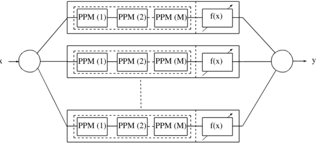
The main limitation of the ambiguity decomposition is that it can be applied only to linearly weighted regression problems and it needs to define in advance a set of optimal weights as well as a set of models that are both accurate and diverse. Depending on the type of the base predictors, whether they are similar or different, ensemble learning can be classified into: homogenous ensembles and heterogeneous ensembles (hybrid ensembles) (Whalen and Pandey (2013) and Wo´zniak et al. (2014)). In homogenous ensembles the base predictors are all of the same type, for example all the base predictors are Decision Trees (DTs) or Neural Networks (NN). An illustration of this type of ensemble architecture is shown in Figure 2.4. On the other hand, in heterogeneous ensembles, models of
> PPM (2) PPM (1) > PPM (2) PPM (1) > PPM (2) PPM (1) - - y x f(x) f(x) f(x) PPM (M) PPM (M) PPM (M)
Figure 2.4:An illustration for a homogeneous ensemble consisting of multiple predictors of the same type
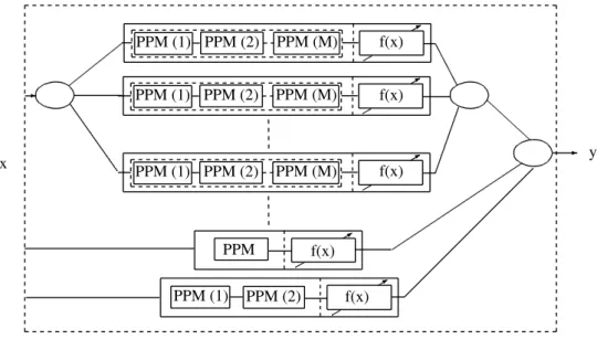
various types are combined to provide the final prediction of the system. There are a number of challenges associated with this type of predictive systems. These challenges include (Wo´zniak et al. (2014)): a) choosing the appropriate models to be combined, b) tuning the models parameters and understanding the effect these parameters have on the individual models performance as well as on the overall performance of the system, and c) choosing the appropriate combining method for the base predictors. The final prediction can be obtained using either selection or fusion methods (Woods et al. (1997) and Kuncheva (2004)). In classifier selection, the base predictors are trained on local regions of the feature space. The locality
of the data can be determined using a number of metrics such as distance metric, correlation or mutual information among others. Depending on the metric used, the final prediction of such ensemble can be obtained from one or more predictors (Bloch (1996) and Roli et al. (2001)). On the other hand, in classifier fusion, the outputs of all the base predictor ares considered in the final prediction, examples of this approach are bagging and boosting methods. Figure 2.5 shows a simple example of heterogeneous ensemble.
-* PPM (2) PPM (1) 3 PPM x * y PPM (2) PPM (1) PPM (M) * PPM (2) PPM (1) PPM (M) * PPM (2) PPM (1) PPM (M) f(x) f(x) f(x) f(x) f(x)
Figure 2.5: An illustration for a heterogeneous ensemble consisting of multiple predic-tors of different types
A more complex architecture of heterogeneous ensembles is to have a pool of com-peting, possibly complex predictors. In this case, multiple predictive systems of different complexities and types are organised in a pool of competing solutions. The predictors can have varying complexities from single predictors to MLMCPS systems. An illustration of this architecture is shown in Figure 2.6.
* 3 * * * P P Mj P P Mj P P Mj > > > P P Mj P P Mj P P Mj > ˆ Y X Predictor (1) Predictor (2) Predictor (M) ˆ fi(x) ˆ fi(x) P P M1 P P M1 P P M1 P P M1 P P M2 P P M2 P P M2 P P M2 ˆ f1(x) ˆ f2(x) ˆ f(x) ˆ f(x) ˆ f(x) P P M P P M ˆ f1(x) ˆ f2(x) P P M1 P P M2 P P M2 P P M2 P P M1 P P M1 Selector Combiner/
2.3
Predictive Systems Evaluation
The performance of both single model and ensemble architecture can be evaluated based on a number of criteria. These criteria include: accuracy, complexity, robustness, adaptation and transparency. This section considers these criteria and their most common well-known measures.
2.3.1
Accuracy
The accuracy of prediction can be calculated, depending on the prediction problem using one of the following measures.
• Numerical measures:
The following points summarise the main measures for calculating the error E (Hyndman and Koehler (2006)):
1. Mean Square Error (MSE):
M SE = 1 N N X i=1 (ˆyi−yi)2 (2.11)
2. Root Mean Square Error (RMSE):
RM SE = √2 M SE (2.12)
3. Sum of Square Regression (SSR):
SSR=
N
X
i=1
(ˆyi−yi)2 (2.13)
4. Mean Absolute Error (MAE):
M AE = 1 N N X i=1 |(ˆyi−yi)| (2.14)
5. Mean Absolute Percentage Error (MAPE): M AP E = 100% N N X i=1 | (ˆyi−yi) yi | (2.15)
6. Root Mean Square Percentage Error (RMSPA):
RM SP E = 2 v u u t[ 100% N N X i=1 (ˆyi−yi) yi ]2 (2.16)
Measures 1-4 are scale-dependent measures, since they depend on the scale of the data. They are mainly used to compare different algorithms applied to the same data set or to data sets of similar scales. Nevertheless, these measures should not be used when the predictive systems are compared across data-sets of different scales. On the other hand, measures 5 and 6 are scale-independent and often used to compare algorithms across different data-sets. However, both measures 5 and 6 are undefined or infinite when the actual output is zero, since the error will be divided by zero in this case.
• Confusion matrix:
Confusion matrix (or contingency table) is a table that illustrates the classification performance of the predictive system. Table 2.1 shows the confusion matrix of a binary classification problem (Alpaydin (2014)).
Table 2.1:Confusion matrix for binary classification problems actual positive actual negative
predicted positive True Positive (TP) False Negative (FN) predicted negative False positive (FP) True Negative (TN)
Assuming that there are two classes: positive class and negative class, the elements shown in the above matrix are (Alpaydin (2014) and Fawcett (2006)):
TN (True Negatives) is the number of examples correctly classified as negatives.
FP (False positives) is the number of negative examples incorrectly classified as positives.
FN (False negatives) is the number of positive examples incorrectly classified as negatives.
For this problem the classification error can be calculated using the following equa-tion:
E = F P +F N
F P +F N +T P +T N (2.17) Several metrics can be derived from the confusion matrix, such as:
Precision Also known as the positive predictive value (PPV). It measures the num-ber of the correctly classified positives divided by the total numnum-ber of positive examples.
P recision= T P
T P +F P (2.18)
Recall Also known as the sensitivity, it measures the proportion of the positive examples that are correctly identified.
Recall = T P
T P +F N (2.19)
Specificity It measures how well the classifier detects the negative examples.
Specif icity = T N
T N +F P (2.20)
F-measure (F-score) is an accuracy test that can be calculated using a weighted average of the precision and recall as shown in the following equation:
F −measure= 2× precision×recall
precision+recall (2.21)
The best value a classifier can achieve in this measure is1and the worst value is0.
When the number of classes (k) exceeds2; the confusion matrix becomes a(k×k)
matrix (Alpaydin (2014)). The main diagonal of the matrix contains the correctly classified examples and the off diagonal elements contain the examples that are
misclassified. Ideally all off-diagonal elements should be0.
• ROC and AUC:
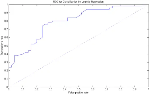
Receiver Operating Characteristic (ROC) is a 2-dimensional graph used to vi-sualise the classifier performance in binary classification problems (Kubat et al. (1998)). Figure 2.7 shows an example of the ROC curve, where the y-axis of this graph represent theT Prate (recall) and the x-axis of the graph represent theF Prate
(1−specif icity). This curve maintains a trade-off between the benefits (true
pos-itives) and the cost (false pospos-itives). An Ideal classifier will have a T Prate = 1
andF Prate = 0. The closer the classifier is to the upper-left corner the better is its
accuracy.
Figure 2.7: The ROC curve for classifying the Virginica class in the Fisher iris data set using logistic regression
The worst case in binary classification is when the classifier performance lies on the main diagonal. In such a case it will have an accuracy value of 50%. However, the performance of classifiers that go below the main diagonal can be improved by flipping their decision (Alpaydin (2014)). In order to obtain a single value that represents the accuracy of the classifier, the Area Under the Curve (AUC) is calculated. An ideal classifier will have an AUC=1.
• Weighted accuracy (cost sensitive) measures:
As explained before, the confusion matrix distinguishes different types of error. In some applications different costs are associated with misclassification errors. For instance, the cost of misclassifying a simple injury as deadly is much lower than the cost of misclassifying a deadly injury as a simple one (King et al. (1995)). For such applications a cost matrix is constructed. This matrix provides the cost of each type of error. For example, the cost matrix of a binary classification problem is given as:
actual positive actual negative predicted positive Cost(0,0) Cost(0,1)
predicted negative Cost(1,0) Cost(1,1)
The optimal prediction in this case can be calculated using the following equation (Elkan (2001)):
L(c, i) =X
j
P(j |c)Cost(i, j) (2.22) Where L is a function which calculates the loss, i is the index for the predicted class,j is the index of the true class,P(j|c)is the probability of the classj being the true classc, andCost(i, j)is the cost of the prediction.
2.3.2
Complexity
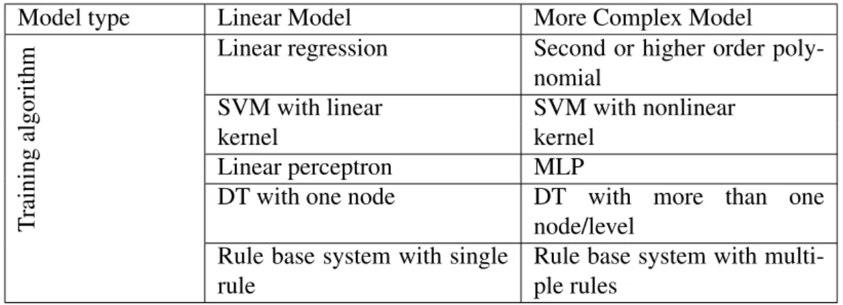
Complexity can be divided into two categories: model complexity and algorithmic com-plexity (Russell and Norvig (2010)). Model comcom-plexity is the comcom-plexity of the final trained model, which can be obtained using different training algorithms. On the other hand, the algorithmic complexity is the complexity of the algorithm used to train the model. The following discussion highlights the differences between these two concepts. Consider Table 2.2, the second column shows various types of predictive models that can be trained to fit a linearly separable classification problem. Though the generated models are all linear models, however, their complexities and the complexities of their training algorithms are widely varied. Increasing the complexity of the classification problem (as shown in the third column) will require changes in the complexities of the models as well as their training algorithms. The algorithmic complexity of the training model plays an
Table 2.2: Learning methods used to generate linear and quadratic predictive Models Model type Linear Model More Complex Model
T
raining
algorithm
Linear regression Second or higher order poly-nomial
SVM with linear SVM with nonlinear
kernel kernel
Linear perceptron MLP
DT with one node DT with more than one node/level
Rule base system with single rule
Rule base system with multi-ple rules
important role in dynamic environments, as the model may need to be retrained repeat-edly.
Meanwhile, the complexity of the developed model should be chosen such that a com-plex model is not chosen for a problem that can be solved using a simpler model (Blumer et al. (1987)).
Figure 2.8 shows an example where three functions of different complexities are used to model a given data set. The first function is a simple linear fit, and it represents the case where the model has lower complexity than what the application requires. The middle function shows a model with moderate complexity and it shows a good representation of the data. Finally the third function shows a model that has higher complexity level than what the application requires.
Figure 2.8: A data set fitted with three functions of increasing complexity. Adopted from Gunn (2012).
2.3.2.1 Algorithmic Complexity Measures
• Kolmogorov complexity
Though Kolmogorov complexity is a theoretically well-defined method for mea-suring the algorithmic complexity, it is not applicable in practise. This method defines the complexity of an algorithm as the length of the shortest Turing machine program that can represent this algorithm. The Kolmogorov complexity is given below (Jankowski and Grabczewski (2011)):
Ωk(P r) =minpr(l(P r) : program pr prints Pr) (2.23)
Where Ωk(P r) represents the Kolmogorov complexity and l(P r) represent the
length of the program. Nevertheless, the search space for this problem is unlimited and the program execution time is also unlimited, which makes finding the pro-gram with the shortest length an unsolvable problem. This is known as the halting problem and can be stated as (Reed (2005)):
”Given a description of an arbitrary computer program, decide whether the program finishes running or continues to run forever”
• Levin Universal Search (LUS)
LUS introduces a time-bound on the Kolmogorov complexity and by that it intro-duces a computable version of the Kolmogorov complexity, the LUS equation is (Jankowski and Grabczewski (2011)):
Ωl(P r) = minpr(l(P r) : program pr prints pr intpr) (2.24) Ωl(P r) =l(P r) +log(tpr) (2.25)
Wheretpris the time required to finish the program.
Nevertheless, solving the LUS is an NP-hard (Non-deterministic Polynomial-time hard) problem, where, an NP problem is a problem for which a solution can be verified in polynomial time using a deterministic Turing machine. Meanwhile, an NP-hard problem is a class of problems which are at least as hard as the hardest problem in NP. Due to this, in practise it is impossible to find the exact solution for this optimisation problem (Jankowski and Grabczewski (2011)).
• Asymptotic analysis and big O notation