w or k i ng pa p ers
14 | 2011
May 2011
The analyses, opinions and fi ndings of these papers
represent the views of the authors, they are not necessarily those of the Banco de Portugal or the Eurosystem
RATIONAL VS. PROFESSIONAL FORECASTS
João Valle e Azevedo João Tovar Jalles
Please address correspondence to João Valle e Azevedo Banco de Portugal, Economics and Research Department
Av. Almirante Reis 71, 1150-012 Lisboa, Portugal; Tel.: 351 21 313 0163, email: [email protected]
BANCO DE PORTUGAL Av. Almirante Reis, 71 1150-012 Lisboa www.bportugal.pt
Edition
Economics and Research Department Pre-press and Distribution Administrative Services Department Documentation, Editing and Museum Division Editing and Publishing Unit
Printing
Administrative Services Department Logistics Division Lisbon, May 2011 Number of copies 150 ISBN 978-989-678-083-8 ISSN 0870-0117 (print) ISSN 2182-0422 (online) Legal Deposit no. 3664/83
Rational vs. Professional Forecasts
∗
Jo˜
ao Valle e Azevedo
†Banco de Portugal Universidade NOVA de Lisboa
Jo˜
ao Tovar Jalles
‡University of Cambridge
May 2, 2011
Abstract
We compare theoretical and empirical forecasts computed by rational agents living in a model economy to those produced by professional forecasters. We focus on the variance of the prediction errors as a function of the forecast horizon and analyze the speed with which it converges to a constant (which can be seen as a measure of the speed of convergence of the economy to the steady state). We look at a standard sticky-prices-wages model, con-cluding that it delivers a strong theoretical forecastability of the variables under scrutiny, at odds with the data (professional forecasts). The flexible prices-wages version delivers a forecastability closer to the data and performs relatively better empirically (with actual data), but mainly because forecasts deviate little from the unconditional mean. These re-sults can be interpreted in at least two ways: first, actual deviations from the steady-state
∗Acknowledgements: The authors are grateful to Valerio Ercolani, Ant´onio Antunes, Nikolay Iskrev, Pedro
Teles, Isabel Correia, Bernardino Ad˜ao, Andrew C. Harvey, Petra Geraats, Mikhail Pranovich, Eva Ortega,
Gabriel Perez-Quiros, James Costain, Samuel Hurtado, Juan Francisco Jimeno, Javier Ortega and Michael Ben-Gad for insightful comments and suggestions as well as seminar participants at the University of Cambridge,
Banco de Portugal, Banco de Espa˜na, University of Birmingham, University of Liverpool and City University
London. The usual disclaimer applies. Most research was done while Jo˜ao Tovar Jalles was a Visiting Researcher
at the Banco de Portugal, whose hospitality is greatly appreciated. The views expressed are those of the authors and do not necessarily represent those of the Banco de Portugal or the Eurosystem.
†Corresponding author: Banco de Portugal, Research Department, Av. Almirante Reis, 71-6th floor,
1150-012 Lisboa, Portugal. E-mail: [email protected]
‡University of Cambridge, Faculty of Economics, Sidgwick Avenue, CB3 9DD, Cambridge UK. E-mail:
are not persistent, in which case the implications of the specific formulation of nominal rigidities for short-run dynamics are unrealistic; second, and still looking through the lens of a model, exogenous (or unmodelled) steady-state shifts attributable to, e.g., changes in monetary-policy, taxation, regulation or in the growth of the technological frontier, occur in such a way as to strongly limit the performance of professional forecasters.
JEL Classification: C32, C53, C68, E12, E13,E17
Keywords: Survey of Professional Forecasters, Green Book forecasts, DSGE models, Nom-inal rigidities
1
Introduction
Despite tremendous efforts over the past decades, macroeconomic forecasting seems as difficult as before. For most variables forecast accuracy is low, simple models prove hard to beat and sophisticated statistical methods provide marginal (if any) improvements at long horizons. This degree of uncertainty should perhaps be considered a feature of the economy, as the same difficulty characterizes professional forecasts (say, from the Philadelphia Survey of Professional Forecasters, henceforth Phil-SPF, the Federal Reserve Green Book, Fed Green-Book, or the European Central Bank Survey of Professional Forecasters, ECB-SPF). Still, there is clear evidence they rank very well in comparison with various statistical methods, being less prone to the structural instabilities of macroeconomic time series (e.g., Faust and Wright, 2007 and Bernanke and Boivin, 2003 for evidence on Green-Book forecasts or Ang, Bakeart and Wei, 2007 for Phil-SPF inflation forecasts). Moreover, professional forecasts can be seen as a fortunate aggregation of various individual forecasts that probably adapt fast to changes in the economy, each using different data, different methods and even some judgment. The question we address is whether the behavior of these forecasts shares characteristics of theoretical and empirical forecasts produced by typical dynamic stochastic general equilibrium (DSGE) models. We will call the first set of forecasts “Professional” and the latter “Rational”.
We view Professional forecasts as the best publicly available proxy for the forecasts pro-duced by well-informed agents in the economy, providing a natural benchmark against which to confront the forecasts produced by rational agents living in a model economy that is taken seriously. Departing from the common practice of comparing moments and impulse response functions, we assess the fit of models to data by analyzing the differences in the relative per-formance of Rational vs. Professional forecasts, paying special attention to the variance of the forecast errors as a function of the forecast horizon as well as to the speed with which it converges to a constant (the speed with which the forecasts converge to the unconditional mean of the variables under scrutiny). Under the strong assumption that unmodelled features of the economy affecting the steady-state are unimportant for the analysis of short-run dynamics, we
can view this exercise as useful to understand in which dimensions (or for which variables) theoretical models provide a reasonable description of the process (or speed) of convergence of the economy to the steady-state. We will interpret small differences in forecast accuracy (as a function of the forecast horizon) in the two worlds (Rational and Professional) as sign that the model is able to replicate an important dimension of actual data.
Our benchmark model economy will be the one discussed in Smets and Wouters (2007) in its New-Keynesian (NK) and Real Business Cycle (RBC) versions (i.e., with and without nominal rigidities). The comparison of the two paradigms is instructive. In fact, nominal rigidities (along with real features adding persistence such as habit formation and investment adjustment costs) are often incorporated with the justification that they enable the models to replicate the persistence of the response to various shocks identified with VAR’s, i.e., impulse response functions that are still “alive” after two or even three years horizons. This translates into theoretical forecastability of the corresponding variables at very long horizons. However, we conclude that for the growth of real variables such as consumption, investment or output, Professional forecasters don’t do better than the mean at horizons greater than 3 or 4 quarters. The notable exception occurs with the unemployment rate (which we take as a proxy for hours worked in the theoretical model). For nominal interest rates both forecasters and agents that live in a sticky-prices-wages economy can form forecasts that are superior to the mean at very long horizons (in practice, simple time series models also can do that due to the very high persistence of nominal rates). For inflation, forecasters still add to the mean after 5 quarters, but little, whereas the standard sticky-price-wage model (under standard parametrizations) is still far from the mean of the process at long horizons, clearly at odds with the data. The RBC version is silent with respect to nominal interest rates and inflation but delivers forecasts of real variables that are closer (in terms of relative performance with respect to the unconditional mean and speed of convergence) to Professional forecasts. The notable exception relates to hours. Once we use these models to forecast actual data, the performance is extremely weak but less so with the RBC version (mainly because forecasts converge to the unconditional mean more rapidly). Again, the exception to this pattern is found with hours/unemployment.
The remainder of the paper is organized as follows: Section 2 shows that, for a host of variables, the predictive power of Professional forecasts vanishes fast as the forecast horizon increases, i.e., the gains (if any) that one obtains by using these forecasts instead of a (real-time) estimate of the unconditional mean of the variables are small. Section 3 confronts these facts with the theoretical and empirical performance of a standard DSGE model, whereas section 4 pays special attention to what occurs during recessions. Section 5 concludes.
2
Professional Forecasts: how much they deliver
Here we assess the predictive power of U.S. Professional forecasts, measuring simply their performance relative to an estimate of the unconditional mean of the variables analyzed.1 In this way we investigate how informative these forecasts are and until when (in terms of forecast horizon) they provide relevant signal relative to what can be viewed as a steady-state forecast.
2.1
Data
We analyze 15 macroeconomic indicators from the Phil-SPF,2 namely: Nominal GNP/GDP (NOUTPUT), Real GNP/GDP (ROUTPUT), Industrial Production Index - Total (IPT), Real Personal Consumption Expenditures - Total (RCON), Net Exports (NETEXP), GDP deflator (GDPDEF), Consumer Price Index (CPI), Real Gross Private Domestic Investment – Resi-dential (RINVRESID), Real Gross Private Domestic Investment – NonresiResi-dential (RINVBF), Real Government Consumption and Gross Investment – State and Local (RGLS), Real Gov-ernment Consumption and Gross Investment – Federal (RGF), Housing Starts (HSTARTS), unemployment (UNRATE), T-bill (TB3MS), T-bond (GS10). We look only at point forecasts and define these as the median forecast in every release of the survey (results with the mean
1Analysis of the forecast performance of Phil-SPF is routinely conducted at the Federal Reserve Bank of
Philadelphia, see Stark (2010) for a recent discussion.
2For complete information on the survey’s background see
http://www.philadelphiafed.org/research-and-data/real-time-center/survey-of-professional-forecasters/spf-documentation.pdf as well as Zarnowitz (1969), Zarnowitz and Braun (1993) and Croushore (1993).
forecast are very similar). The individual respondent’s point forecasts are generally close to the central tendencies of their subjective distributions (e.g., Engelberg et al. 2009) while there is clear evidence that this aggregation produces forecasts that are in general superior to individual forecasts. Obviously, a not so straightforward aggregation can result in forecast improvements, and this can be achieved even when there is (as in Phil-SPF) entry and exit of forecasters, see Capistr´an and Timmerman (2009).
Regarding the Fed Green-Book, we analyze predictions for real GDP (ROUTPUT) and GDP deflator (GDPDEF) only, and only those constructed with approximately the same information set as Phil-SPF’s (i.e., presented at the FOMC meeting closest to the middle of the second month of a given quarter). The sample periods are as follows: Phil-SPF, 1981q3-2009q2; Fed Green-Book, 1981q3-2003q4.3 All data is firstly aggregated quarterly when necessary (to be
consistent with the variables forecasted in the Phil-SPF) and except for unemployment and interest rates, all data is in growth rates. For a more detailed description of data treatment and transformations please refer to Appendix A.
2.2
Methodology
We begin our analysis by taking the real-time vintage data from 1968q4 through 1981q3 -h
quarters, for h = 1, ...,5.4 We then estimate the unconditional mean of the variables under scrutiny by simply computing the average of each variable for this vintage, which is our bench-mark forecast for 1981q3. As a reference, we also compute forecasts from an estimated Direct Autoregression (AR) using data through 1981q3 -h. We repeat this procedure using the vintage from 1968q4 through 1981q4 -h, h= 1, ...,5 and so forth until 2009q2. It should be noted that most variables are available with a delay of one quarter. Hence, to properly compare these benchmark forecasts with Phil-SPF and the Fed-Green Book forecasts we re-label the forecast horizon so that the information sets with each method approximately coincide (so, the h step
3The Fed Green-Book only releases forecasts every five years and 2003 is the latest available year with data.
4These series were retrieved from the Philadelphia Fed website.
http://www.phil.frb.org/research-and-data/real-time-center/real-time-data/data-files/. See, e.g., Croushore and Stark (2001, 2003) for a discussion of real-time data.
ahead, with 0 ≤ h ≤ 4, Phil-SPF and Green-Book forecasts will be considered as h+ 1 step ahead forecasts since the latest observation of the variable to be forecasted does not in general refer to the forecast moment,5 which is approximately the middle of the quarter since at least
1990q3).6
We then compare the forecast accuracy of the Professional predictions, AR and also real-time average by computing the ratio of Root Mean Square Forecast Error (RMSFE) of both the AR and Professional forecasts relative to that of the benchmark forecast (real-time average). It should be noted that the forecast error is defined as the difference between the forecast and the corresponding observation of the latest vintage of data available (considering the h
quarters ahead vintage alters little the results, at least in relative terms, see also Stark 2010 for a thorough analysis of this issue). Following Fair and Shiller (1989) we also run the following forecast encompassing regression:
yt+h =α+β0ftreal+h +β1ftx+h+εt+h (1)
where yt+h is the observation of the variable forecasted, freal is the forecast from the real-time
average,fx is the forecast from the candidate modelx, in our case either the AR process or the Professional forecasts andεt+h is a (most likely serially correlated) regression error. Obviously,
if β1 ̸= 0, then forecasts from candidate model x add information relative to the real-time
average. Both the RMSFE ratios and the β1 coefficients are computed and presented for the
full sample as well as for an aggregation of recession quarters as defined by the NBER (results for each decade, that is, the 1980s, 1990s and the period 2000q1-2009q2 are available upon request).
Additionally, we will take a closer look at Phil-SPF and Fed-Green Book forecasts for real GDP (ROUTPUT) and the GDP deflator (GDPDEF), to understand if Phil-SPF forecasts represent best practice, or close to best practice, within professional forecasts. In fact, using
5This does not apply, e.g., to interest rates, whose quarterly average is to be forecasted but are obviously
available in the middle of the quarter, when the forecast is made.
6The timing of the previous American Statistical Association/NBER survey (that was taken by the
data until 1991, Romer and Romer (2000) show that the Fed-Green Book forecasts of inflation and real GDP are statistically unbiased and dominate private sector forecasts (i.e., suggesting that the Federal Reserve has considerably more information beyond what is known to the private sector). The period of “Great Moderation”7 between 1982-2007 has affected the
time-series properties of many variables as well as the forecasting performance of different models. In particular, D’Agostino and Whelan (2008) show that the superior forecasting performance of the Fed-Green Book forecasts deteriorated considerably after 1991. Similarly, Gamber and Smith (2008) find that the Fed’s relative forecasting superiority has declined relative to Phil-SPF forecasts for both inflation and real GDP growth after 1994. Thus, and in line with Chong and Hendry (1986) and Granger and Newbold (1986), we will conduct efficiency-type encompassing tests based on the estimation of the following equations:
eftx+h =γ0+γ1(eftB+h−ef x t+h) +εt+h (2) eftB+h =δ0+δ1(eftx+h−ef B t+h) +εt+h (3)
where eftx+h(= yt+h − ftx+h) is a general representation for the alternative x forecast error
(Fed-Green Book or Phil-SPF) whereas efB
t+h(= yt+h −ftB+h) is the benchmark forecast error
(respectively Phil-SPF or Fed-Green Book). Under the null hypothesis that γ1 = 0(δ1 = 0),
fx
t+h(ftB+h) encompasses ftB+h(ftx+h).
It is important to note that a forecast performing as well as an estimate of the unconditional mean in terms of RMSFE (or encompassed by it) may nonetheless be useful if it can more often accurately predict the direction of change in the actual series (Joutz and Stekler, 2000). With this in mind we will examine the sign forecast accuracy of the forecasts by constructing the following two-by-two contingency table in which the actual and forecast data for each quarter are classified (i) by whether the actual change in a given variable is positive (+) or negative/zero (-,0), and (ii) whether the forecast correctly or incorrectly predicted the sign:
7See, e.g., McConnell and Perez-Quiros (2000), Stock and Watson (2003) and Giannone, Lenza and Reichlin
Contingency Table
n11 : ∆yt+h(+),∆ftx+h(+) n12 : ∆yt+h(−,0),∆ftx+h(+) n21: ∆yt+h(+),∆ftx+h(−,0) n22: ∆yt+h(−,0),∆ftx+h(−,0)
where the actual change is ∆yt+h =yt+h−yt and the predicted change is ∆ftx+h = f x
t+h −yt.
Note thatytis the most recent (quarterly) value known at the time of the forecast. The diagonal
cells include numbers of correct sign forecasts and the off-diagonal cells include the numbers of incorrect sign forecasts. In testing the null hypothesis of no association between the frequency of actual and predicted changes we use Fisher’s exact test.
2.3
Results and Discussion
2.3.1 Forecast Accuracy
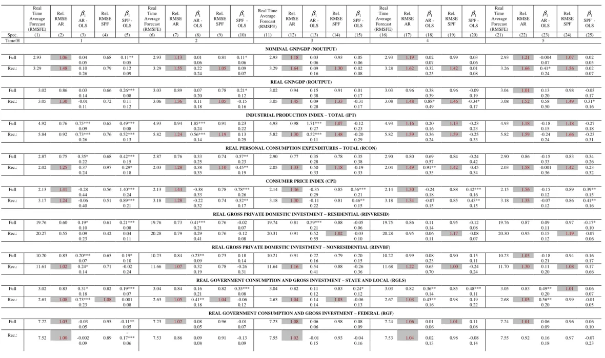
Our main empirical results regarding forecast accuracy are presented in Tables 1.1 and 1.2 for the Phil-SPF and the Fed-Green Book, respectively.8 Table 1.1 presents the forecast perfor-mance with respect to the 15 macroeconomic variables defined before. It contains the ratio of the Root Mean Square Forecast Error (RMSFE) of both the AR and Professional forecasts rel-ative to the benchmark forecast (real-time average) as well as the estimate of β1 resulting from
OLS estimation of Eq. (1) at different forecast horizons (robust standard errors are reported below the estimated coefficient).9 The main conclusions from Table 1.1 follow:
- considering the full sample, Phil-SPF forecasts add signal relative to the benchmark (real-time average) only up to h= 2 when looking at the significance of the β1 coefficients for
most variables under scrutiny. The exceptions are Phil-SPF’s CPI inflation, GDP deflator, unemployment and interest rates (both T-bond and T-bill rates) predictions throughout
8For reasons of parsimony, these are condensed tables that focus solely on the full sample and recession
periods that result from simple aggregation of all periods corresponding to the 4 recessions identified by the NBER. Versions of these tables with sub-samples are available from the authors upon request.
9It is advisable to use Newey-West standard errors since the error terms are generally serially correlated
and heteroskedastic. For further details see Harding and Pagan (2006). Other estimators could have been used instead, e.g., the method outlined in Kiefer and Vogelsang (2002) and Phillips et al. (2003).
the different forecast horizons and Phil-SPF’s RGLS (State and Local Government Con-sumption and Gross investment growth) up to h= 4.
- considering the full sample, the relative (to the real-time average) RMSFE for Phil-SPF’s forecasts is clearly less than one for all horizons only in the case of unemployment, interest rates and, in a lesser extent, inflation (CPI and GDP deflator). In the case of 10 year bond interest rates the AR outperforms Phil-SPF whereas for the 3-month T-bill rate the opposite is true. For output (nominal and real) and specially industrial production, housing starts and net exports this ratio indicates mostly useless Phil-SPF forecasts at horizons greater than or equal to h = 3. For consumption, investment (residential and non-residential) and Government expenditures (federal and local) there is still some supe-riority on average (relative to the real-time average) at horizonsh= 3,4,5. In these cases however, it would in general suffice to use a simple autoregression as the rel. RMSFE compares favorably with Phil-SPF’s.10
- for all variables except (again) interest rates, inflation (CPI and GDP deflator) and un-employment, Phil-SPF (and AR) forecasts that correspond to recession periods have a quite poor performance relative to the real-time average except at h= 1 (for many vari-ables). Afterwards the rel. RMSFEs are higher than those obtained with the full sample and more frequently well above 1. This evidence is in line with e.g. Zarnowitz (1992) , Zarnowitz and Braun (1992), McNees (1992) and McNees and Ries (1983) who reported a number of systematic errors made by forecasters regarding recession periods. For h= 2,
β1 is nonetheless still significant for Phil-SPF in the case of consumption and for AR
forecasts in the cases of state and local government expenditures, non-residential private investment and industrial production, despite the fact that rel. RMSFE is above 1 in two of the three cases.
10One should bear in mind that regressions including only recession periods contain solely 28 observations
and this fact may be the underlying cause of some marginally significant coefficient estimates for longer forecast horizons in some variables (e.g. nominal and real GDP or residential investment).
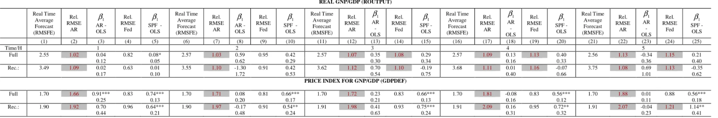
We now focus on Table 1.2 which is organized similarly to Table 1.1 but refers to Fed-Green Book’s predictions instead, computed using the same information set as Phil-SPF forecasts (i.e., we focus on the four quarterly forecasts produced before the FOMC meetings occurring in the middle of a given quarter). In this case the sample size is shorter, going up to 2003q4. We look only at Fed-Green Book’s forecasts of real output and GDP deflator inflation, the ones available from the Federal Reserve Bank of Philadelphia. For real output, the overall performance is worse than the Phil-SPF counterpart in terms of rel. RMSFE,11in accordance with Gavin and Mandal (2003) whose evaluation of real output growth forecasts finds no evidence of the Fed’s superior information about the economy. As for GDP deflator-based inflation, we find relative RMSFEs smaller than unity together with highly significantβ1 coefficients at all forecast horizons for the
full sample. We will later compare in more detail Green book and Phil-SPF forecasts for these variables, to see if Phil-SPF forecasts can be considered best practice among well-informed agents in the economy.
Putting it simply, this exercise shows that for most variables a real-time estimate of the con-ditional mean seems a hard to beat forecast (even) at short horizons. Regarding unemployment, nominal interest rates and inflation, Professional forecasts do contain relevant information be-yond that of our crude benchmark forecast. In these cases, however, it is more clear that the distance between these forecasts and the real-time average forecast is surely overstated, in the sense that the latter is supposed to measure a steady-sate value that may be varying over time (e.g., due to changes in monetary policy or labor market institutions). This is not damaging for our purposes as it allows us to refer to this distance as an upper bound on what a theoretical model (without regime shifts in monetary policy or labor market institutions) ought to deliver in terms of forecast accuracy relative to the steady state forecast.
2.3.2 Sign forecast accuracy
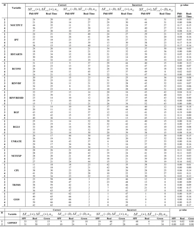
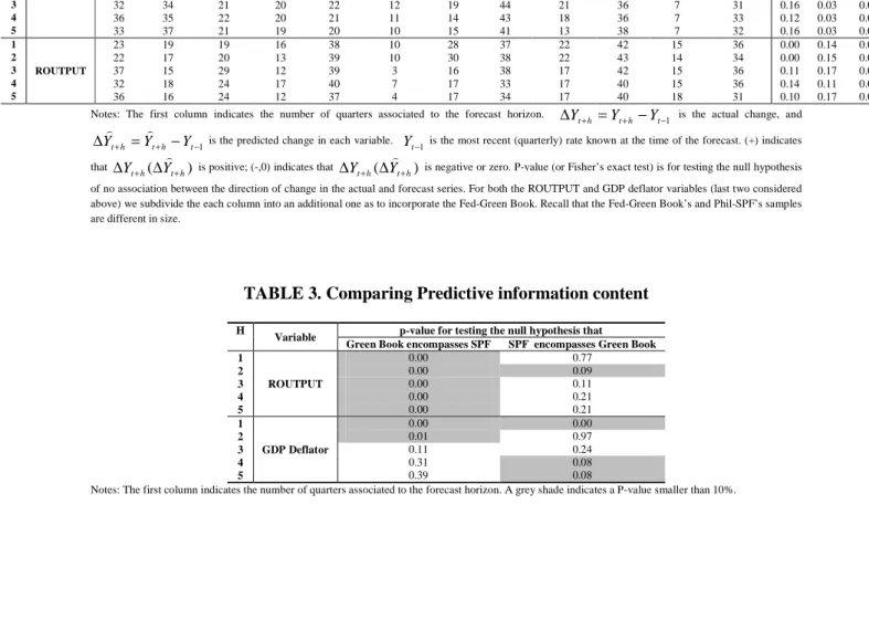
Table 2.1 reports the cell counts for the contingency table described in section 2.2 and p-values for the null of no association between actual and predicted changes for the Phil-SPF,
time average and Fed-Green Book forecasts. First, it is clear that most p-values for Phil-SPF and Green-book forecasts are less than 0.1, or the null hypothesis of no association between actual and predicted changes is rejected, indicating that, in general, these forecasts accurately predict the direction of change in the actual series. What is more interesting for our purposes is to compare the behavior of Professional’s forecasts to that of the benchmark (real-time average) forecast. In fact, it is perfectly possible that this rough benchmark forecast accurately predicts the direction of change at long horizons. First, we observe that for h= 1,2 Phil-SPF and Green Book forecasts are, in general, clearly more informative than the real-time average (lower associated p-values), according to this criterion. Second, for real output Green-book (not Phil-SPF) forecasts clearly look more useful than the benchmark even at h = 3,4,5 .12
But the main result emerging from Table 2.1 is that at horizons greater than h = 2 and for all other variables except interest rates, CPI inflation, unemployment and to a lesser extent State and local Government spending, the null of no association (no valuable prediction of the direction of change) is either rejected for both Phil-SPF, Green-Book and real-time average forecasts or, when the null is not rejected for Phil-SPF and Green-Book forecasts, it is often rejected in the case of real-time average forecasts. All in all, the main message is that (with the exceptions mentioned) Professional forecasts certainly loose marginal informational content when compared to the benchmark after 2/3 quarters, in line with the previous subsection.
2.3.3 Phil-SPF vs. Fed Green-Book
We now compare more carefully Phil-SPF and Green book forecasts to assess wether the former can be recognized as best practice, or close to best practice among professional forecasts. Table 3 reports the p-values for testing γ1 = 0 and δ1 = 0 in Eqs. (4) and (5) with Phil-SPF as the
benchmark, that is, to assess wether Phil-SPF forecasts encompass Fed-Green Book forecasts or vice-versa (with a common sample up to 2003q4). For every forecast horizon in the case of real output, we reject γ1 = 0 but we cannot reject δ1 = 0, indicating that Phil-SPF forecasts
12Recall however that the Fed-Green Book sample is different from he Phil-SPF one. We are still postponing
for this variable embody useful predictive information above that contained in Fed-Green Book forecasts. In the case of GDP deflator inflation the evidence is not clear cut but favors the conclusion that Green book forecasts encompass Phil-SPF forecasts at h= 4,5.
We proceed to an alternative way of comparing the forecast performance of these Professional forecasts by constructing a table with the ratio of MSFEs (Fed-Green Book’s to Phil-SPF’s) for different sample periods with and without recessions. Table 4 reports MSFE ratios for the full sample, an aggregation of recession periods, the sample up to 2001q4 and the sample up to 1991q4 for forecast horizons ranging from h= 1 through h= 5 both for real output growth and GDP deflator inflation.
Focusing on real GDP growth first, we observe that the MSFE ratios are above 1 for short forecast horizons in the various sub-samples that include recessions, implying that Phil-SPF’s forecasts perform superiorly on average. For h= 4,5 the reverse is true, as a result of relatively large Phil-SPF forecast errors in the very beginning of the evaluation period, coinciding with the 1981/82 recession, see below. More generally, if recession periods are excluded from the full sample and both sub-samples, the MSE ratio increases (in general). As for GDP deflator inflation, we observe that Fed-Green Book’s forecasts only perform superiorly when his above 1 and for the samples (that include recessions) ending in 1991q4 and (less so) 2001q4 (the exception occurs with h = 5, due to Fed-Green Book’s substantially larger errors from 1983 through 1989, see below). The general superiority observed in these earlier sub-samples clearly vanishes with the inclusion of more recent data. To test the significance of superior predictive ability, each MSFE ratio entry is matched with the p-value from a modified Diebold-Mariano (1995) test. The null hypothesis is that Fed-Green Book’s and Phil-SPF’s forecasts have equal predictive accuracy. Now, for both variables most p-values are above 10% when h = 3,4,5, suggesting that even though the MSFE is more often lower for Phil-SPF, the differences in forecast accuracy are not significant. More frequent exceptions to this pattern are found at very short horizons (h= 1,2) and favoring Phil-SPF’s predictions.
We now move to a graphical comparison of the performance of Fed-Green Book’s and Phil-SPF’s predictions of real output growth and GDP deflator inflation. Figures 1.a-i show in the
upper panel 1-year (4 quarters) moving averages of squared forecast errors (Rolling-SFEs, with the last observation of the moving average in thexaxis) and also (bottom panel) the cumulative squared forecast errors (from 1981Q1 trough the date in the x-axis) for the two variables. The grey-shaded regions identify NBER recession periods. First, one can conclude that Rolling-SFE’s rise during business cycle turning points and recessions. Second, for both variables and most forecast horizons we conclude that Fed-Green Book’s forecast errors are generally lower than Phil-SPF’s (albeit similar) up until the early 1990s (the exceptions occurs with output growth when h= 1,2 and GDP deflator inflation when h= 1); in general, after this point we observe that the series of accumulated squared forecast errors get close and eventually cross (whenever the Phil-SPF series is above that of the Fed-Green book initially; when this did not occur, as with GDP growth with h = 1,2 and GDP deflator inflation when h = 1, the series drift farther apart). All this clearly indicates an overall relative deterioration of Fed-Green book’s forecasts.
All in all, it seems fair to conclude that at least for these two variables Phil-SPF’s forecasts are not inferior to Fed-Green Book’s. In the remainder of the paper we will focus almost exclusively on Phil-SPF forecasts, regarding them as a good proxy of the forecasts produced by well-informed agents in the economy.
3
How does a Standard DSGE model forecast?
3.1
The model
We move now towards the core of the paper, comparing previous results with the theoretical and empirical forecast performance of the medium-scale model analyzed and estimated in Smets and Wouters (2007) (henceforth SW07), based on Smets and Wouters (2003) and Christiano et al. (2005). The model has many of the features now popular in the growing so-called DSGE literature13 including monopolistic competition in the goods and labour markets, ingredients
aimed at improving the fit of the model to observables such as habit formation in consumption, investment adjustment costs, variable capacity utilization (all of these implying amplification of the effects of shocks) and crucially, nominal frictions such as Calvo sticky prices and wages along with partial backward-looking indexation. Monetary policy follows a Taylor rule and has real effects when nominal frictions are important. Seven shocks are included (total factor productivity, investment productivity, monetary policy, government spending and risk premium following an AR(1) process along with price and wage markup shocks following an ARMA(1, 1) process) as well as seven observables: output, investment, consumption, wages (all in log differences) as well as inflation, nominal interest rates and (log of) hours. Further details can be found in Appendix B.
We start by solving a first order log-linear approximation of the model using the algorithm of Swanson et al. (2004). We then build the state space representation of the solution, including measurement equations linking deviations from the steady-state (or first differences of deviations from the steady-state whenever observed data is non-stationary) to the (quarterly) observables: (log differences of) output, consumption, investment, wages , (log of) hours and (levels of) nominal interest rate and inflation. We use exactly the same data treatment as in SW07, implying that the match between the model’s variables and Phil-SPF’s counterparts is not perfect. Specifically, SW07 observables for output, consumption, investment and wages are expressed in per capita (working age population) terms and nominal interest rates are measured with the Federal funds rate (quite close to the 3-month T-bill rate from Phil-SPF nonetheless). The inflation measure in the model is GDP deflator inflation (i.e., perfect match with Phil-SPF) whereas (minus) Phil-SPF’s unemployment, while following closely hours, surely drifts somehow from the concept in the model.
We analyze the forecast performance of two versions of SW07: the original one featuring nominal rigidities, or New-Keynesian (NK) version, and another where we shut down these rigidities (i.e., flexible prices or RBC version, where we further reduce the observables by eliminating inflation and nominal interest rates while keeping the wage markup shock). We use Smets and Wouters’s estimated parameters (mode of the posterior distribution, obtained from
combining the likelihood function with a set of independent priors for 36 of the 41 structural parameters included in the model. The other 5 parameters are fixed) using data from 1984q1 through 2004q2 (see details in Appendix B14). We choose this sample to avoid quibbles regarding
the onset of the “Great Moderation” and likely changes in monetary policy within the period starting in 1966q1 (SW07’s beginning of the sample). We arguably go against the RBC version by not re-estimating the model, i.e., we keep fixed the structural parameters not related to nominal rigidities. Forecasts of the observables are just conditional expectations given the state-space model and are obtained with the Kalman filter, which is also used to derive the theoretical covariance matrix of the forecast errors for various horizons.15
We start with a theoretical analysis of the forecastability of the various variables implied by the model , i.e., we assume the model is the economy and derive analytically the standard deviation of the forecast errors at various horizons.16 The (artificial) sample size is set at
T = 160 (thinking in 40 years of post war quarterly data), although it could be lower given the fact that the Kalman filter converges fast. Figure 2 presents the theoretical relative (to the standard deviation of the variables) root mean squared forecast error (RMSFE) for output, consumption, investment, inflation, hours, nominal interest rate and wages of the original SW07 (NK version). As easily seen, for nominal interest rates, inflation but also hours, there is a very strong predictability at short horizons, the relative RMSFE converges slowly and after 20 quarters this ratio is still around 0.4 for inflation and nominal interest rates and 0.7 for hours. For consumption, output and investment the initial level lies around 0.45-0.55 but convergence is fast except for investment. Wages is the least predictable variable, with a relative RMSFE starting around 0.8. All this means that a rational agent understanding this economy should
14Results for the empirical and theoretical forecast performance across all the variations considered in SW07
(i.e., shutting off, individually, the various real and nominal frictions) are available upon request. The main conclusions in this paper are robust to these different parametrizations.
15For the theoretical analysis this only implies that agents would be using a minimum mean square criterion
if they were to pick this as a point forecast, i.e., they know the parameters of the model and produce conditional expectations given the state space model. Regarding the empirical analysis in the paper, it is fair to say that Bayesian estimation of the models would make natural using as point forecasts the mean of the predictive density of future observations, see e.g., Adolfson, Lind´e, and Villani (2007).
16Here and in the rest of the paper, we could have looked as well at the correlation of the forecast errors for
be able to forecast in such a way as to clearly outperform the unconditional mean in the case of hours, inflation, nominal interest rates even at very long horizons. For consumption, output and specially investment, he would clearly beat the mean even at 6 quarters ahead.
In the case of the RBC version (Figure 3) the conclusions are naturally quite different. The model becomes silent with respect to inflation and nominal interest rates but for the remaining variables the convergence of the RMSFE towards the standard deviation of the variables is much faster. For output, the relative RMSFE is around 0.8 for 1-step ahead forecasts and above 0.9 afterwards. For consumption and investment the speed of convergence is lower but clearly higher than that of the sticky prices/wages version. For wages, there is only significant predictability at 1-step ahead whereas for hours convergence of the RMSFE towards the standard deviation is slow but at a level clearly above that of the NK version. Now, it is important to note that this feature of the specific NK model analyzed here is certainly common to any model featuring price and wage setting frictions along with an important indexation mechanism (to target or current inflation or a combination of the two) aimed at rationalizing the observed persistence of inflation, see e.g., the models in Christiano et al. (2005), Adolfson et al. (2007), Ireland (2007) or Schorfheide (2005). This occurs because indexation generates high persistence in inflation and in other variables (and thus strong forecastability). In other way, any deviation of inflation from target in this kind of world represents a persistent (forecastable) deviation of the economy from its steady-state.
3.2
Model vs. Data
Here we confront the results in section 2, regarding Phil-SPF’s forecasts, with the theoretical and empirical forecast accuracy of the NK and RBC versions of SW07 analyzed above. To be clear, we view the relative (to the standard deviation) RMSFE of well-informed agents in the economy (Professional forecasters), as a statistic that should be matched by a realistic DSGE model, just as it should deliver steady-state ratios, volatilities and correlations that are close to what is observed in the data. E.g., if this relative RMSFE for output growth at 1 quarter
horizon is 0.3 in the model and 0.8 in the case of Professional forecasters (data), we view this as an indication that the model delivers a forecastability that is at odds with the data. And similarly if after 10 quarters the Rational agent living in the model economy is still able to clearly outperform the mean whereas Professional forecasters don’t. Comparison of Professional and Rational (given the model) forecasts can thus inform theory or at least show the limitations of the theoretical models, even though the mapping from Rational to Professional forecasts may be considered loose.
If nothing else, we believe Professional forecasts allow us to measure how fast (from the perspective of the forecasters) the economy is moving towards the steady-state. Specifically, we can measure this convergence to the steady-state through the speed with which the RMSFE converges to the standard deviation of the variables. In fact, if after some time (horizon) the forecast is (on average) very close to the unconditional mean of the variable under scrutiny, this means the forecaster believes the economy (or at least that variable) takes that much time to reach the steady-state (in the absence of unpredictable shocks). With rational expectations this must be a characteristic of the process generating the data.17
Now, results in the previous section suggest that for most real variables (and in particular output, investment and consumption) Professional forecasts lose grip after 2 quarters, meaning that using as forecast an estimate of the unconditional mean of the variables does not imply losing valuable information. Professional forecasts of unemployment and nominal interest rates are still clearly superior to the mean after one year whereas for inflation (CPI and GDP) there is forecastability but in a lesser extent. Notice further that we are using as benchmark a real-time estimate of the mean. If this mean is time-varying or shifts occasionally, e.g., if the steady-state changes due to permanent changes in taxation or in monetary policy (that changes for instance target inflation), the real-time average will not be efficient whereas professional forecasters are probably aware of these shifts. This is useful for our purposes as it allows us to interpret the relative RMSFE of Professional forecasts (which is thus deflated) as a lower bound on what
17We are certainly aware of the difficulty of characterizing as rational a consensus (mean or median) forecast,
see e.g., Bonham and Cohen (2001). Rationality should arguably be analysed at the individual level but exit and entry of forecasters in the surveys makes this a difficult task.
a realistic theoretical model (without steady-state shifts) ought to deliver in terms of forecast accuracy relative to the steady-state forecast. Similarly then, in the mapping from Professional forecasts to the theoretical performance of SW07, we must see the model as corrected for regime changes, hence we cannot be as demanding when using the models in a pseudo out-of sample forecasting exercise with actual data.
Table 5 compares the results, for the theoretical and empirical (with actual data) relative (to the standard deviation) RMSFE of the NK and RBC versions of SW07, vis-a-vis that obtained with Phil-SPF forecasts. In the analysis of the empirical performance we focus on the sample 1981q3- 2009q2 (coinciding with the previous SPF’s evaluation sample). If we take first the theoretical rel. RMSFE for output and investment, it is clear that the distance between the rel. RMSFE of Phil-SPF and that of the theoretical model is in general smaller for the RBC model, clearly so for all h in the case of investment and for h = 3,4,5 in the case of output. At h = 1,2 in the case of output, the RBC has a clearly lower forecastability. This result for output and investment contrasts to what obtains with the NK version, where the strong predictability at h = 1 and even at long horizons is at odds with Phil-SPF. In the case of consumption the RBC is more successful at matching the data when h= 1,2, whereas for h = 3,4,5 the evidence favors the NK version (notice however that it may well be the case that the rel. RMSFE obtained with Phil-SPF may not be statistically different from 1). With respect to hours/unemployment (we recall that Phil-SPF forecasts unemployment, which explains nonetheless around 80% of the variation in hours), the RBC is closer to Phil-SPF at all horizons, although the rel. RMSFE is consistently above that of Phil-SPF for h >2. This is in clear contrast with the strong predictability implied by the NK model. The RBC version is silent with respect to the nominal interest rate and inflation but for the NK model it is clear that while the behavior of the rel. RMSFE function is very close to that of Phil-SPF in the case of nominal interest rates, for inflation the very high forecastability of the NK model does not match data from Phil-SPF forecasts. We notice also that even if the rational agent uses the forecasts produced by the univariate representation of inflation given the model (NK univariate, i.e, using only past inflation to produce the forecast), the strong forecastability of
inflation is almost unchanged. This is a consequence of the degree of backward-looking behavior (indexation) of inflation in the NK model. Once the rational agent observes current inflation and its history, information on other shocks is almost irrelevant to form a close to efficient conditional expectation of inflation at some point in the future. If the model is realistic, this implies that a forecaster would only need to nail the univariate representation of inflation in order to obtain a close to efficient forecast.
Now, demanding from the models forecasts of actual (observed) data changes radically, in absolute terms, the picture above, with a clear deterioration of the empirical counterpart of the statistics above.18 Nonetheless, Table 5 (bottom panel) shows that for real output and investment the RBC is close to Phil-SPF (and dramatically superior to the NK version). For wages (no data for Phil-SPF) the performance of both models is very similar whereas for consumption both the RBC and NK versions have a very weak performance (although the latter performs relatively better at horizons greater than 5 quarters, despite the fact that forecasts are close to the mean). For nominal interest rates the NK model is close to Phil-SPF ath= 1,2 but it drifts quite fast afterwards, becoming useless after 6 quarters (in clear contrast with the theoretical result). For inflation, the empirical performance of the NK model is beyond terrible, a qualification also deserved for the behavior of the RBC version with respect to hours (in this case the NK version is clearly more informative but not much compared to Phil-SPF at h >2). As far as we are aware, only Rubaszek and Skrzypczynski (2008) compared forecasts from a (3 equations prototypical) DSGE model to SPF forecasts while using real-time data for estimation and forecasting (instead of the latest vintage of data and a fixed set of parameters, useful for our purposes). Their sample size is also larger than usual, spanning 1994:q1–2006:q2. The main conclusions are that while for a few horizons in the case of GDP growth the DSGE model seems to outperform SPF (not statistically significant difference in accuracy), in the case of inflation and short-term nominal interest rate SPF clearly outperforms the DSGE model.19
18Again, it is fair to recognize that the literature aknowledges the likely misspecification of DSGE models.
E.g., Del Negro et al. (2007) approximate a DSGE model by a vector autoregression (VAR) and then relax the implied cross-equation restrictions in order to improve fit. It is possible to optimally relax these restrictions and it is found that forecast accuracy improvements obtain.
All in all, the results above suggest that the nominal rigidities apparatus of the NK model, which greatly amplifies the effects of shocks, tended to produce an excessively large theoretical forecastability, extending over long horizons. This seems clearly at odds with the data. The stripped down flexible prices version (RBC) delivers a forecastability resembling more that of the Phil-SPF while performing relatively better empirically (the important exception relates to hours/unemployment). This is due to the fact that deviations from the steady-state tend not to be persistent, hence forecasts (conditional expectations) are closer to the mean of the variables. Thus, not taking risks (or not assuming a detailed knowledge of short-run dynamics) compensated in this context. The RBC model seemed more immune to misspecification (notice also that the RBC version was not even re-estimated, it keeps all the parameters from the estimated NK model).
Next we repeat the analysis for recession periods.
4
How do Rational and Professional Forecasts behave
during Recessions?
There is clear evidence that macroeconomic forecasts fail to predict business-cycle’s turning points and, moreover, forecasting the beginning of a recession one or two quarters in advance never occurred. In this aspect data (professional forecasts) are in line with standard models, where recessions must be seen as the result of large exogenous shocks (or at least unpredictable shocks in size and moment). Hence, one should not demand (or expect) accurate forecasts referred to the first period (quarter) of a recession. Afterwards, the theoretical mechanisms embodied in the models should be helpful in determining the path of observed variables.
Here we show that the conclusions above seem to carry over to recession20 periods, and are certainly magnified. That is, the performance of the NK version of SW07 is quite poor
forecasts from 1996 through 2004, arguing for a positive contribution of the model in some instances (specially for output growth).
20As identified by the NBER dates. For the purposes of this section we include a quarter before and a quarter
compared to that of the RBC version. First, we recall that Professional forecasts (from the Fed-Green Book or SPF) have a poorer (relative to an estimate of the unconditional mean) performance during recession periods (Tables 1.1 and 1.2), specially at horizons greater or equal to 3 quarters. The exceptions occur with inflation and nominal interest rates as well as with housing market variables for short horizons (housing starts and residential investment). Despite this, they are clearly more accurate than model forecasts. To analyze this we simply plot the various forecasts (Fed-Green Book, Phil-SPF, NK and RBC) for h = 1, ...,5 for real GDP growth, inflation and interest rates21(see Figures 4.a-i). Analysis of other real variables conveys a very similar message. As easily seen, Professional forecasts of real GDP have no clue about the beginning and dynamics of recessions with an anticipation of 2 or more quarters (h ≥ 3) whereas 1 quarter earlier they have some signal and for the current quarter they are accurate (h = 1, we recall that one step ahead forecasts in the case of Professional forecasts is really a nowcast). Now, although the RBC model performs poorly relative to professional forecasts, the characterization is very similar. The RBC obviously does not anticipate the recessions but provides signal about subsequent developments when h = 1,2. The performance of the NK model is clearly disastrous, specially during the last recession, where observed deflation and very low nominal interest rates contribute to forecasts that never consider consecutive negative growth (but instead a quick way out of the recession). This is clearly not the case in the 1991 and 2001 recessions. Again, the “defensive” (or not implying persistent deviations from the steady -state) dynamics implicit in the RBC version seems to at least produce forecasts that have some signal (although definitely close to the steady-state, or unconditional mean). For inflation and nominal interest rates we observe that professional forecasts are very accurate at short horizons and convey some signal at longer horizons. For nominal interest rates, the NK model does not produce out of bounds forecasts, but they are weak compared to those of Professionals. For inflation, NK forecasts are very poor and do seem out of bounds, except during the last recession.
5
Concluding remarks
It seems unwise to expect too much from macroeconomic forecasts. For what really matters (real variables, but except for unemployment) best practice has little to say at horizons greater than 2, 3 quarters. If statistics derived from these facts inform general equilibrium modelling, in the sense that a rational agent living in the economy should deduce similar statistics, they probably say the economy has not been deviating persistently from the steady-state. In the theoretical models, this should translate into low forecastability (relative to a naive, or steady-state forecast and, again, except for unemployment - hours) of most variables. This occurs with the RBC version of the model analyzed here but clearly not with the NK version. Furthermore, even recognizing limitations in a model without nominal frictions and (or) limited (not persistent) departures from the steady-state, the fact is that empirical forecasts seem to indicate that the model minimizing type II errors (or less prone to misspecification) is the RBC version. Forecasts are closer to naive (or to steady-state values) but provide some signal. The alternative (relying on a particular description of nominal rigidities) is not reliable. In our view, and given the effects of the inclusion of nominal frictions on forecast performance (theoretical and empirical), care should be taken at least on the way trend inflation (or varying central bank target) is modeled. In the model analyzed here and many others, the central bank target (steady-state inflation) is fixed, which implies that any deviation of inflation from target is necessarily interpreted by the model as a deviation from the steady-state (inflation gap). We are persuaded by Cogley and Sbordone’s (2008) analysis that once movements in trend inflation are taken into account, the (backward-looking) indexation component of a general new-Keynesian Phillips curve is not needed to fit the data well. If indexation is incorrectly assumed, it implies a supposedly high theoretical forecastability of inflation (even if a rational agent only looks past inflation) as we have shown. This is clearly at odds with the data (Professional forecasts) and does not survive a forecast evaluation with actual data. Another interpretation of the results rests on the observation that theoretical models used to fit several decades of data are likely missing relevant changes in monetary policy, product and labor market regulation, taxation or in the
trend growth of technology. If these changes are reasonably unpredictable, there is potential compatibility between professional forecasters having a hard time and the NK model becoming seriously misspecified only along those dimensions, i.e., nominal rigidities can play an important role which is hidden due to lack of control for what can be seen as steady-state shifts.
References
[1] Adolfson, M., J. Lind´e and M. Villani (2007). “Forecasting Performance of an Open Economy DSGE Model”, Econometric Reviews, 26: 289–328.
[2] Adolfson, M., S. Las´een, J. Lind´e and M. Villani (2007). “Bayesian Estimation of an Open Economy DSGE Model with Incomplete Pass-Through”, Journal of International Economics, 72:481–511.
[3] Adolfson, M., S. Las´een, J. Lind´e and M. Villani (2008). “Evaluating an Estimated New Keynesian Small Open Economy Model”, Journal of Economic Dynamics and Control, 32: 2690–2721.
[4] Ang, A., Bekaer, G. and M. Wei. (2007). “Do Macro Variables, Asset Markets, or Surveys Forecast Inflation Better?”, Journal of Monetary Economics, 54(4): 1163-1212.
[5] Bernanke, B.S. and J. Boivin (2003). “Monetary Policy in a Data-Rich Environment”, Journal of Monetary Economics, 50: 525-546.
[6] Bonham, C. and R. H. Cohen (2001). “To Aggregate, Pool, or Neither: Testing the Rational Expectations Hypothesis Using Survey Forecasts,” Journal of Business and Economic Statistics, 19(3): 278-91.
[7] Capistr´an, C. and A. Timmermann (2009). “Forecast Combination with Entry and Exit of Ex-perts.” Journal of Business and Economic Statistics, 27: 428-440.
[8] Chong, Y. Y. and D. F. Hendry (1986). “Econometric evaluation of linear macroeconometric models”. Review of Economic Studies, 53, 671–690.
[9] Christiano, L., Eichenbaum, M. and C. Evans (2005). “Nominal rigidities and the dynamic effects of a shock to monetary policy.” Journal of Political Economy, 113 (1): 1-45.
[10] Christiano, L. J., Trabandt, M. and K. Walentin (2009). “Introducing Financial Frictions and Unemployment into a Small Open Economy Model”, Sveriges Riksbank Working Paper Series No. 214.
[11] Cogley, T. and Sbordone, A. M. (2008). ”Trend Inflation, Indexation, and Inflation Persistence in the New Keynesian Phillips Curve”, American Economic Review, 98(5): 2101-26.
[12] Croushore, D. and T. Stark (2001). “A Real-Time Data Set for Macroeconomists”, Journal of Econometrics, 105:111-130.
[13] Croushore, D. and T. Stark (2003). “A Real-Time Data Set for Macroeconomists: Does the Data Vintage Matter?” Review of Economics and Statistics 85:605–617.
[14] Croushore, D. (1993). “The Survey of Professional Forecasters”, Business Review, Federal Reserve Bank of Philadelphia, November/December, 3-15.
[15] Croushore, D. (2006). “An evaluation of inflation forecasts from surveys using real-time data”, Working Paper No. 06-19, Federal Reserve Bank of Philadelphia.
[16] D’Agostino, A. and K. Whelan (2008). “Federal Reserve information during the Great Modera-tion”, Journal of the European Economic Association, 6(2-3): 609-620.
[17] Del Negro, M., Schorfheide, F., Smets, F. and R. Wouters (2007). “On the Fit of New Keynesian Models”, Journal of Business and Economic Statistics, 25: 123-143
[18] Diebold, F. X. and R. S. Mariano (1995). “Comparing predictive accuracy”, Journal of Business and Economic Statistics, 13:252-263.
[19] Edge, R. M., Kiley, M. T. and J. P. Laforte (2010). “A comparison of forecast performance be-tween Federal Reserve staff forecasts, simple reduced-form models, and a DSGE model”, Journal of Applied Econometrics, 25(4): 720-754
[20] Engelberg, J., Manski, C. F. and J. Williams (2009). “Comparing the Point Predictions and Sub-jective Probability Distributions of Professional Forecasters”, Journal of Business and Economic Statistics, 27: 30-41.
[21] Fair, R. C. and R. J. Shiller (1989). “The Informational Context of Ex Ante Forecasts”, The Review of Economics and Statistics, 71(2): 325-31
[22] Faust, J. and J. H. Wright (2007). “Comparing Greenbook and Reduced Form Forecasts using a Large Realtime Dataset”, NBER Working Papers 13397
[23] Faust, J. and J. H. Wright (2008). “Efficient forecast tests for conditional policy forecasts”, Journal of Econometrics, 146(2), 293-303.
[24] Gamber, E. and J. Smith (2009). “Are the Fed’s inflation forecasts still superior to the the Private Sector’s?”, Journal of Macroeconomics, 31(2): 240-251.
[25] Garcia, J. (2003). “An introduction to the ECB’s Survey of Professional Forecasters”, ECB Occasional Paper, No.8, September.
[26] Gavin, W. T. and R. J. Mandal, (2003). “Evaluating FOMC forecasts”, International Journal of Forecasting, 19: 655–667.
[27] Giannone, D., Lenza, M. and L. Reichlin (2008). “Explaining The Great Moderation: It Is Not The Shocks”, Journal of the European Economic Association, 6(2-3), pp. 621-633
[28] Harding, D. and A. Pagan (2006). “Synchronization of cycles”, Journal of Econometrics, 132(1), 59-79.
[29] Ireland, Peter N. (2007). “Changes in the Federal Reserve’s Inflation Target:Causes and Conse-quences” Journal of Money, Credit and Banking, 39(8): 1851-2110.
[30] Granger, C. W. J. and P. Newbold (1986). Forecasting economic time series (2nd ed.). London: Academic Press.
[31] Joutz, F. and H. O. Stekler, (2000). “An evaluation of the predictions of the Federal Reserve”, International Journal of Forecasting, 16, 17–38.
[32] Kiefer, N. and T. Vogelsang (2002). “Heteroskedasticity autocorrelation robust standard errors using the Bartlett kernel without truncation”, Econometrica 70: 2093–2095.
[33] McConnell, M. and G. Perez-Quiros (2000).“Output Fluctuations in the United States: What Has Changed Since the Early 1980’s?”, American Economic Review, 90 (5): 1464-1476
[34] McNees, S.K., (1992), “How large are economic forecast errors?” New England Economic Review, Jul/Aug 25–33.
[35] McNees, S.K. and J. Ries (1983). “The track record of macroeconomic forecasts”. New England Economic Review, Nov/Dec 5–18.
[36] Phillips, P.C.B., Sun, Y. and S. Jin (2003). “Consistent HAC Estimation and Robust Regression Testing when using Sharp Original Kernels with no Truncation”, Cowles Foundation for Economic Research, Yale University.
[37] Romer, C. and D. Romer (2000), “Federal Reserve information and the behaviour of interest rates”, American Economic Review, 90: 429-457.
[38] Rubaszek, M., and P. Skrzypczynski (2008). “On the Forecasting Performance of a Small-Scale DSGE Model,” International Journal of Forecasting, 24: 498-512.
[39] Schorfheide, F. (2005). “Learning and monetary policy shifts.” Review of Economic Dynamics, 8(2): 392-419.
[40] Smets, F. and R. Wouters (2003). “An Estimated Dynamic Stochastic General Equilibrium Model of the Euro Area”, Journal of the European Economic Association, 1(5): 1123-1175.
[41] Smets, F. and R. Wouters. (2007). “Shocks and Frictions in US Business Cycles: A Bayesian DSGE Approach”, American Economic Review, 97(3): 586-606.
[42] Stark, T. (2010). “Realistic evaluation of real-time forecasts in the Survey of Professional Fore-casters”, Federal Reserve Bank of Philadelphia, Research Rap Special Report, May 2010
[43] Stock, J.H. and M.W. Watson (2003). “Has the Business Cycle Changed and Why?,” NBER Chapters, in: NBER Macroeconomics Annual 2002, Vol17, pp 159-230, National Bureau of Eco-nomic Research
[44] Stock, J.H., and M.W. Watson (2007). “Why Has U.S. Inflation Become Harder to. Forecast?”, Journal of Money, Credit, and Banking, 39:3-34
[45] Swanson, E., Anderson, G. and A. Levin (2005). “Higher-Order Perturbation Solutions to Dy-namic, Discrete-Time Rational Expectations Models”, mimeo, Federal Reserve Bank of San Fran-sisco.
[46] Zarnowitz, V. (1969). “The new ASA-NBER Survey of Forecasts by Economic Statisticians”, American Statistitican, 23: 12-16.
[47] Zarnowitz, V., (1992). Business cycles: Theory, history, indicators and forecasting. In: National Bureau of Economic Research Studies in Business Cycles, vol. 27. University of Chicago Press, Chicago.
[48] Zarnowitz, V., Braun, P., (1992). Twenty two years of the NBER-ASA Quarterly Outlook Sur-veys: Aspects and comparisons of forecasting performance. NBER Working Paper 3965, New York.
[49] Zarnowtiz, V. and Braun, P. (1993). Twenty-Two years of the NBER-ASA Quarterly Economic Outlook Surveys: Aspects and comparisons of forecasting performance, in J.H. Stock and M.W. Watson (eds.), Business Cycles, Indicators and Forecasting (NBER Studies in Business Cycles, Volume 28), 11-84, Chicago: University of Chicago Press.
Appendix A - Variables’ definitions and sources
Our data for both the Phil-SPF and Green-Book predictions comes directly from the Fed-eral Reserve Bank of Philadelphia website and covers the period 1968:q4-2009:q222; The latest vintage of all series (against which forecasts are compared) was downloaded from the FRED database (Federal Reserve Bank of St. Louis). Data is converted to quarterly whenever the series are available at a higher frequency (by averaging the observations within each quarter ). Except for unemployment and interest rates, all data is in growth rates. Except for interest rates, all published data is seasonally adjusted, in accordance with the targets of Professional’s forecasts. Prior to 1992, nominal and real output forecasts refer to nominal GNP. GDP deflator forecasts refer to GNP deflator prior to 1992, to GDP deflator from 1992 through 1995 and to chain-weighted price index for GDP since 1996.
The following table shows the definition of all series, Phil-SPF’s andFRED’s id code, and observation range.
Definition FRED code SPF code
Gross Domestic Product (Nominal) GDP NOUTPUT
Gross Domestic Product (Real) GDPC1 ROUTPUT
Real Personal Consumption Expenditures PCECC96 RCONS
Real Private Nonresidential Fixed Investment PNFIC96 RINVBF
Real Private Residential Fixed Investment PRFIC96 RINVRESID
Housing Starts Total: New Privately Owned Housing Units HOUST HSTARTS
Industrial Production Index INDPRO IPT
Real Federal Cons. Exp. & Gross Investment FGCEC1 RGF
Real State & LocalCons. Exp. & Gross Investment SLCEC1 RGLS
Net Exports of Goods & Services NETEXP NETEXP
Civilian Unemployment Rate UNRATE UNRATE
Consumer Price Index: All Items CPIAUCSL CPI
Gross Domestic Product Deflator GDPDEF GDPDEF
10-Year Treasury Constant Maturity Rate GS10 GS10
3-Month Treasury Bill: Secondary Market Rate TB3MS TB3MS
As for data used in SW07, we note that the latest available vintage of the following series is used: FRED’s GDPC1 (real output), PCECC96 (consumption) and PNFIC96 (investment),
22http://www.phil.frb.org/econ/spf/spfpage.html. For a recent discussion about the Phil-SPF see Croushore
(2006). For a recent discussion on differences between surveys, do refer to Engelberg et al. (2007) and Clements (2008).
which are divided by the Bureau of Labor Statistics (BLS) series LNU00000000Q (Civilian noninstitutional population, 16 years and over). Short term nominal interest rate is the Fed-eral funds rate (FRED’s FEDFUNDS), inflation is measured with FRED’s GDPDEF (perfect match with SPF), hours worked is obtained as average weekly hours (nonfarm business, BLS’s PRS8500602) multiplied by civilian employment (16 and over, FRED’s CE16OV) and then di-vided by BLS’s series LNU00000000Q (Civilian noninstitutional population, 16 years and over)
Appendix B - Smets and Wouters (2007) model
Table 1
Log-linearized equations of the SW07 model (sticky-price-wage economy) (1) yt=cyct+iyit+rksskyzt+εgt (2) ct= λ/γ 1 +λ/γct−1+ 1 1 +λ/γ Etct+1+ wsslss(σ c−1) cssσ c(1 +λ/γ) (lt−Etlt+1) − 1−λ/γ (1+λ/γ)σc(rt−Etπt+1)− 1−λ/γ (1+λλ/γ)σcε b t (3) it = 1+βγ1(1−σc)it−1+ βγ (1−σc) 1+βγ(1−σc) Etit+1+ φγ2(1+βγ1(1−σc))qt+εit (4) qt=β(1−δ)γ−σcEtqt+1−rt+ Etπt+1+ (1−β(1−δ)γ−σc) Etrtk+1−εbt (5) yt=ϕp(αkst + (1−α)lt+εat) (6) ks t =kt−1+zt (7) zt = 1−ψψrkt (8) kt = (1−δ)/γkt−1+ (1−(1−δ)/γ)it+ (1−(1−δ)/γ)φγ2(1 +βγ(1−σc))εit (9) µpt =α(ks t −lt)−wt+εat (10) πt= βγ (1−σc) 1+ιpβγ(1−σc) Etπt+1+ ιp 1+βγ1−σcιpπt−1− (1−βγ(1−σc)ξ p)(1−ξp) (1+ιpβγ(1−σc))(1+(ϕp−1)εp)ξpµ p t +ε p t (11) rk t =lt+wt−kt (12) µwt =wt−σllt−1−1λ/γ(ct−λ/γct−1) (13) wt= βγ (1−σc) 1+βγ(1−σc)(Etwt+1+ Etπt+1) + 1 1+βγ(1−σc)(wt−1+ιwπt−1)− 1+βγ(1−σc)ι w 1+βγ(1−σc) πt − (1−βγ(1−σc)ξ w)(1−ξw) (1+βγ(1−σc))(1+(ϕ w−1)εw)ξwµ w t +εwt (14) rt=ρrt−1+ (1−ρ)(rππt+ry(yt−yt∗)) +r△y((yt−yt∗)−(yt−1 −yt∗−1)) +εrt (15) εa t =ρaεat−1+ηta (16) εbt =ρaεbt−1 +ηbt (17) εgt =ρgεat−1+ρgaηat +η g t (18) εi t =ρIεIt−1+ηIt (19) εrt =ρrεrt−1 +ηrt (20) εpt =ρpεpt−1+η p t −µpηpt−1 (21) εw t =ρwεwt−1+ηwt −µwηwt−1
Note: The model variables are: output (yt), consumption (ct), investment (it), utilized and
installed capital (ks
t, kt), capacity utilization (zt), rental rate of capital (rkt), Tobin’sq(qt),
price and wage markup (µpt, µw
t), inflation rate(πt), real wage (wt), total hours worked (lt),
and nominal interest rate (rt). The shocks are: total factor productivity (εat),
investment-specific technology (εi
t), government purchases (ε g
t), risk premium (εbt), monetary
policy (εr
t), wage markup (εwt) and price markup (ε p t).