Using dry and wet year hydroclimatic extremes to guide future hydrologic projections

(1)

www.hydrol-earth-syst-sci.net/20/2811/2016/ doi:10.5194/hess-20-2811-2016

Using dry and wet year hydroclimatic extremes to guide future

hydrologic projections

Stephen Oni1,5, Martyn Futter2, Jose Ledesma2, Claudia Teutschbein3, Jim Buttle4, and Hjalmar Laudon1

1_{Department of Forest Ecol. Manage., Swedish University of Agricultural Sciences, 901 83, Umeå, Sweden}

2_{Department of Aquatic Sciences and Assessment, Swedish University of Agricultural Sciences, 750 07, Uppsala, Sweden} 3_{Department of Earth Sciences, Uppsala University, Villavagen 16, 752 36, Uppsala, Sweden}

4_{Department of Geography, Trent University, 1600 West Bank Drive, Peterborough, ON, K9J 7B8, Canada} 5_{Department of Biology, Trent University, 1600 West Bank Drive, Peterborough, ON, K9J 7B8, Canada} Correspondence to:Stephen Oni ([email protected])

Received: 7 January 2016 – Published in Hydrol. Earth Syst. Sci. Discuss.: 20 January 2016 Revised: 21 June 2016 – Accepted: 22 June 2016 – Published: 13 July 2016

Abstract.There are growing numbers of studies on climate change impacts on forest hydrology, but limited attempts have been made to use current hydroclimatic variabilities to constrain projections of future climatic conditions. Here we used historical wet and dry years as a proxy for ex-pected future extreme conditions in a boreal catchment. We showed that runoff could be underestimated by at least 35 % when dry year parameterizations were used for wet year con-ditions. Uncertainty analysis showed that behavioural pa-rameter sets from wet and dry years separated mainly on precipitation-related parameters and to a lesser extent on pa-rameters related to landscape processes, while uncertainties inherent in climate models (as opposed to differences in cali-bration or performance metrics) appeared to drive the overall uncertainty in runoff projections under dry and wet hydrocli-matic conditions. Hydrologic model calibration for climate impact studies could be based on years that closely approx-imate anticipated conditions to better constrain uncertainty in projecting extreme conditions in boreal and temperate re-gions.

1 Introduction

There are growing numbers of studies on climate change im-pacts on watershed hydrology, but these are usually based on long-time series that depict average system behaviour (Bo-nan, 2008; Lindner et al., 2010: Tetzlaff et al., 2013). As a re-sult, limited attempts have been made to use extreme dry and

wet conditions to assess plausible future conditions. Increas-ing numbers of studies are showIncreas-ing the importance of ensem-ble projections to create a matrix of possiensem-ble futures, where the mean provides a statistically more reliable estimate than can be obtained from a single realization of possible future conditions (Bosshard et al., 2013; Dosio and Paruolo, 2011; Oni et al., 2014a; Räty et al., 2014). However, the predic-tive uncertainty of precipitation projections is still larger than that for temperature (Teutschbein and Siebert, 2012). This inherent uncertainty might further increase in the warmer fu-ture as precipitation dynamics become less consistent due to a shift in winter precipitation patterns toward rainfall domi-nance (Berghuijs et al., 2014; Dore, 2005).

It is unequivocally believed that climate is a first-order control on watershed hydrology (Oni et al., 2015a, b; Vörös-marty et al., 2000). Although climate change is a global phe-nomenon (IPCC, 2007), it will likely also alter local catch-ment water balances (Oni et al., 2014b; Porporato et al., 2004). Prolongation of drought regimes or increasing fre-quency of storm events observed in different parts of the world (Dai, 2011; Trenberth, 2012) calls for greater attention on how to constrain uncertainty in predicting extreme dry and wet conditions. While the frequency of hydroclimatic extremes might be low under present-day conditions (Wellen et al., 2014), there could be intensification of precipitation events globally as climate changes (Chou et al., 2013). Oth-erwise, preparations for the future could be undermined by our inability to properly simulate or project new conditions outside our current modelling conditions.

(2)

Models are useful tools in hydrology and runoff has be-come a central feature in the modelling community to as-sess cumulative impacts (Futter et al., 2014; Lindström et al., 2010). Hydrological modelling has benefitted immensely from the use of long-term runoff series from monitoring pro-grammes to gain insights into change in fundamental sys-tem behaviour (Karlsson et al., 2014) and to aid our under-standing of watershed responses to both short- and long-term environmental changes (Wellen et al., 2014). While con-ceptualization of many of these hydrologic models is based on average natural rainfall–runoff processes derived from long-term series, both simple and complex models still per-formed well in simulating long-term dynamics at the water-shed scale (Breuer et al., 2009; Li et al., 2015; Vansteenkiste et al., 2014a). Growing complexity in hydrologic models has led to increasing equifinality (Beven, 2006) due to multi-dimensionality of compensatory parameter spaces. However, extensive explorations of parameter spaces in complex mod-els have also helped to gain further insights into system be-haviour beyond simple models.

Uncertainty in model predictions depends on the length of time series used for calibration and validation (Larssen et al., 2007). Despite strong arguments against the use of the term “validation” (Oreskes et al., 1994), it is still a norm in the hydrologic modelling community to calibrate to one condi-tion and reevaluate the model in different condicondi-tions (Cao et al., 2006; Donigian, 2002; Wilby, 2005). This has made split-sample testing a popular way of assessing the internal working process of a model in hydrologic study (Klemeš, 1986) to ensure that the model is not tuned or over-parameterized before embarking on future projections. While modelling staged under this framework is usually based on average system conditions depicted by long-term series, it may not fully reflect processes operating under very dry and wet hydroclimatic conditions. This can also be due in part to inherent structural uncertainties in models (Butts et al., 2004; Refsgaard et al., 2006; Vansteenkiste et al., 2014b) that can stem from conceptualization, scaling and connectivity of processes between the landscape mosaic patches of a water-shed that the models are representing (Tetzlaff et al., 2008; Ren and Henderson-Seller, 2006). This is the case in Karls-son et al. (2014) that showed increasingly large predictive uncertainty when their model was tested on over a century long record due to non-stationarity of the historical series. It is therefore inevitable that this level of uncertainty will be amplified when projected into the unknown future where, unlike at present, we have no data to confirm our findings (Refsgaard et al., 2014). However, no consensus has yet been reached regarding whether the uncertainty due to differences in hydrologic model structures and/or calibration strategies would be greater than the unresolved uncertainty inherent in climate models when projecting hydrologic conditions in bo-real or temperate ecozones.

One way to constrain the uncertainty in hydroclimatic pro-jections is to utilize historical wet and dry years as a proxy

for the future conditions expected as climate changes. This is analogous to differential split-sample test previously used (Coron et al., 2012; Klemeš, 1986; Seibert, 2003; Refsgaard and Knudsen, 1996), but is less commonly used in hydrol-ogy (Andréassian et al., 2014; Refsgaard et al., 2014). Here we used hydrological and meteorological observations in dry and wet years in a long-term monitored headwater catchment in northern Sweden. The objectives of this study were to (1) utilize long-term field observations in Svartberget to gain insights into hydroclimatic behaviour in dry and wet years as a proxy to future climate extremes and (2) quantify the un-certainty in our current predictive practices that is based on such long-term series. Such uncertainty quantification will allow us to assess the limitations and uncertainties in hydro-logical model-based climate change impact analysis related to the hydrological model calibration strategies and to com-pare these with the uncertainty related to the climate models.

2 Data and method 2.1 Study site

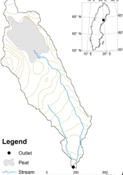
This modelling exercise was carried out in Svartberget (64◦160N, 19◦460E), a 50 ha headwater boreal catchment within the Krycklan experimental research infrastructure in northern Sweden (Fig. 1) (Laudon et al., 2013). Modelling results presented here were based on the long-time series of precipitation, air temperature and runoff (1981–2012) from a weather and flow monitoring station at the outlet of Svart-berget. Svartberget has two headwater streams, one of which drains a completely forest landscape, while the other drains a headwater mire. The catchment has a long-term mean an-nual temperature of about 1.8◦_{C with minimum (January)}

and maximum (July) mean monthly temperatures of −9.5 and 14.5◦C. The catchment receives a mean annual precipi-tation of 610±109 mm with more than 30 % falling as snow (Laudon and Ottosson-Löfvenius, 2015). Snow cover usually lasts from November to May (Oni et al., 2013). The catch-ment has a long-term mean annual runoff of 320±97 mm with subsurface pathways dominating runoff delivery to streams. Spring melt represents the dominant runoff event in the catchment and lasts 4 to 6 weeks. Forest cover includes a century old Norway spruce (Picea abies) and Scots pine (Pinus sylvestris) with some deciduous birch species (Betula spp.). Sphagnum sp.dominates the mire landscape and ri-parian zones (Ledesma et al., 2016). Svartberget has gneis-sic bedrock overlain by compact till of about 30 m thickness to the bedrock. The catchment elevation ranges from 114 to 405 m above sea level and was delineated using a digital ele-vation model (DEM) and lidar (Laudon et al., 2013). 2.2 Climate models

We used 15 different regional climate models (RCMs) from the ENSEMBLES project (Van der Linden and Mitchell,

(3)

Table 1.List of RCMs from the EU ENSEMBLES project used in this study and their respective driving GCMs.

No. Institute RCM Driving GCM

1 C4I RCA3 HadCM3Q16

2 CNRM Aladin ARPEGE

3 DMI HIRHAM5 ARPEGE

4 DMI HIRHAM5 BCM

5 DMI HIRHAM5 ECHAM5

6 ETHZ CLM HadCM3Q0

7 HC HadRM3Q0 HadCM3Q0

10 ICTP RegCM ECHAM5

11 KNMI RACMO ECHAM5

12 MPI REMO ECHAM5

13 SMHI RCA BCM

14 SMHI RCA ECHAM5

15 SMHI RCA HadCM3Q3

2009, Table 1). All RCMs had a resolution of 25 km and were based on Special Report on Emission Scenario (SRES) A1B emission scenarios. The SRES A1B represents a balanced growth of economy and greenhouse gas emission in the fu-ture (IPCC, 2007). The old greenhouse gas scenario (SRES based) became outdated in the meantime; the new Represen-tative Concentration Pathway (RCP) based scenarios could have been used in current climate change impact studies. However, because the focus of this paper lies on the method-ology rather than on the impact results, it is acceptable to rely on an old SRES scenario in line with our other recent studies in this region (Jungqvist et al., 2014; Oni et al., 2014, 2015b). Precipitation and temperature values (2061–2090) were ob-tained by averaging the values of the RCM grid cell with centre coordinates closest to the centre of the catchment and of its eight neighbouring grid cells. Due to systematic biases in RCM data and the spatial disparity between the RCM grid cell and a small catchment like Svartberget, post-processing of RCM data is required (Teutschbein and Seibert, 2012; Ehret et al., 2012; Muerth et al., 2013). The distribution map-ping method (Ines and Hansen, 2006; Boe et al., 2007) was used for bias correction of the 15 RCM-simulated precip-itation and air temperature series on monthly bases using data from a weather station (1981–2010) located within the Svartberget catchment. This was achieved by adjusting the theoretical cumulative distribution function (CDF) of RCM-simulated control runs (1981–2010) to match the observed CDF. The same transformation was then applied to adjust the RCM-simulated scenario runs for the future (2061–2090). As some RCMs tend to simulate a large number of days with low precipitation (e.g. drizzle) instead of dry conditions, we applied a specific precipitation threshold to prevent consid-erable alteration of the distribution. RCM bias corrections

Figure 1.Svartberget, a long-term monitored headwater catchment in the northern boreal ecozone of Sweden. The catchment (50 ha) drains terrestrial area consisting of forest (82 %) and upland mire (18 %). Streamflow measurements were taken at the downstream confluence point.

presented here were fully described in Jungqvist et al. (2014) and Oni et al. (2014, 2015b).

2.3 Modelling and analysis

The Precipitation, Evapotranspiraton and Runoff Simulator for Solute Transport (PERSiST) is a semi-distributed bucket-type rainfall–runoff model with a flexibility that allows mod-ellers to specify the routing of water following the percep-tual understanding of their landscapes (Futter et al., 2014). This feature makes PERSiST a useful tool for simulating streamflow from landscape mosaic patches at a watershed scale. The model operates on a daily timescale with inputs of precipitation and air temperature. The spatial interface re-quires an estimate of area, land cover proportion and reach length/width of the hydrologic response units. In the PER-SiST application presented here, we used three buckets to represent the hydrology of Svartberget. These include snow, upper soil and lower soil buckets. In the snow routine bucket, the model utilized a simple degree day evapotranspiration and degree day melt factor (Futter et al., 2014). Although the maximum rate of evapotranspiration could be independent of wet and dry years as used in this study, the actual rate of evap-otranspiration could be influenced by the amount of water in the soil and by an evapotranspiration (ET) adjustment param-eter. The latter is an exponent for limiting evapotranspiration that adjusts the rate of evapotranspiration (depending on

(4)

wa-0 100 200 300 400 500 600 700 800 1 91 181 271 361

Pr

ec

ip

ita

tio

n

(m

m

)

Dry year Wet year 0 100 200 300 400 500 600 700 800 1 91 181 271 361

Ru

no

ff

(m

m

)

Dry year Wet year (a) ( b )

Figure 2.Cumulative plots of(a)precipitation and(b)runoff in dry (1995, 2002, 2005 and 2010) and wet (1987, 1992, 2000 and 2001) hydrologic years. The hydrologic year is 1 September (day 1) to August 31 of the following year (day 365). The cumulative plots shown here represent the average for all the dry and wet years noted above.

ter depth in the bucket or how much is evapotranspired). The snow threshold partitions precipitation as either rain or snow. The model also simulates canopy interception for snowfall and rainfall to the uppermost bucket. In the modelling anal-ysis presented here, we used three buckets to generate runoff processes in Svartberget. The quick flow bucket simulates surface or direct runoff in response to the inputs of rainfall or snowfall depending on antecedent soil moisture status. The runoff generation process was partitioned between the quick flow and lower soil buckets (upper and lower) following the square matrix described in Table 2.

We utilized Monte Carlo analysis to explore parameter spaces using a range of parameter values listed in Table 3. The evapotranspiration adjustment parameter sets the rate at which ET can occur when the soil is no longer able to generate runoff, and this was set to 1 in the upper soil box. Maximum capacity is the field capacity of the soil that deter-mines the maximum soil water content held. The time

con-Table 2.Square matrix used to partition runoff generation between buckets in the PERSiST application presented here. For example, we conceptualized that 40 % of the precipitation inputs are retained in the upper box, 60 % are transferred to the lower box and 0 % are transferred to the groundwater (row 1).

Upper box Lower box Groundwater

Upper box 0.4 0.6 0

Lower box 0 0.5 0.5

Groundwater 0 0 1

stant specifies the rate of water drainage from a bucket and requires a value of at least 1 in PERSiST. The relative area index determines the fraction of area covered by the bucket and is also set to 1 for our simulations. Infiltration parameters in each bucket determine the rate of water movement through the soil matrix. The model is based on series of first-order dif-ferential equations that are solved sequentially following the bucket order in the square matrix. More detailed information about PERSiST parameterization and equations is provided in Futter et al. (2014).

The model was calibrated against streamflow to generate present-day runoff conditions. Initial manual calibration was performed on the entire time series to minimize the differ-ence between the simulated and observed runoff based on Nash–Sutcliffe (NS) statistics. The manual calibration also helped to identify a suite of parameter ranges to be used in the Monte Carlo analysis by varying each parameter value following steps listed in Futter et al. (2014). The Monte Carlo tool works in such a way that the model was calibrated on NS-1 in line with other works (Senatore et al., 2011; Mas-caro et al., 2013), so that the NS value for the overall period of simulation tends toward 1. This helped to determine the ranges to use in the subsequent Monte Carlo analysis for the wet and dry year simulations. Starting from a random point, we sampled each parameter space 500 times before jumping to the next space (depending on whether the model perfor-mance was better or worse). We specified 100 iterations dur-ing the initialization of the Monte Carlo tool so that 100 en-sembles of credible parameter sets could be generated. This resulted in 50 000 (500×100) runs. In addition to Nash– Sutcliffe statistics, the Monte Carlo tool also takes note of other metrics during sampling. The Monte Carlo tool utilizes the Metropolis–Hastings algorithm and its mode of operation was described in Futter et al. (2014).

The best parameter sets (100 in this case) were selected based on the highest NS statistics from untransformed/log-transformed data. The parameter sets were also analysed for other metrics such as variance of modelled/observed series (Var), absolute volume difference (AD), root mean square er-ror (RMSE) and coefficient of determination (R2). These top parameter sets derived from the Monte Carlo tool are referred to as behavioural parameters henceforth. The behavioural

(5)

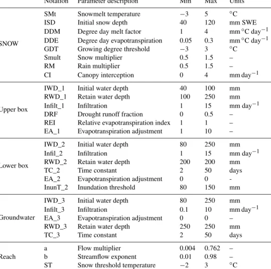
pa-Table 3.Parameter notations, descriptions and ranges used in the Monte Carlo analyses in this study.

Notation Parameter description Min Max Units

SNOW

SMt Snowmelt temperature −3 5 ◦C

ISD Initial snow depth 40 120 mm SWE

DDM Degree day melt factor 1 4 mm◦C day−1

DDE Degree day evapotranspiration 0.05 0.3 mm◦C day−1

GDT Growing degree threshold −3 3 ◦C

Smult Snow multiplier 0.5 1.5 –

RM Rain multiplier 0.5 1.5 –

CI Canopy interception 0 4 mm day−1

Upper box

IWD_1 Initial water depth 40 100 mm

RWD_1 Retain water depth 100 250 mm

Infilt_1 Infiltration 1 15 mm day−1

DRF Drought runoff fraction 0 0.5 –

REI Relative evapotranspiration index 1 1 –

EA_1 Evapotranspiration adjustment 1 10 –

Lower box

Infil_2 Infiltration 1 15 mm day−1

TC_2 Time constant 2 50 days

EA_2 Evapotranspiration adjustment 0 0

-InunT_2 Inundation threshold 80 150 mm

Groundwater

Infilt_3 Infiltration 0.1 10 mm day−1

EA_3 Evapotranspiration adjustment 0 0 –

TC_3 Time constant 2 50 days

Reach

a Flow multiplier 0.004 0.762 –

b Streamflow exponent 0.01 0.98 –

ST Snow threshold temperature −2 3 ◦C

rameters were subjected to further analyses to determine hy-drologic behaviour in dry and wet years. These include the cumulative distribution function (CDF) of behavioural pa-rameters to determine the sensitive papa-rameters and discrimi-nant function analysis (DFA) to determine the domidiscrimi-nant pa-rameter(s) that separate the hydrology of wet from dry years. Wet years were defined as hydrologic years with runoff ex-ceeding 430 mm yr−1 _{or 40 % higher than average annual}

runoff (1995, 2002, 2005 and 2010). Dry years were defined as hydrologic years with runoff less than 150 mm yr−1or less than 50 % of average annual runoff (1987, 1992, 2000 and 2001). The hydrologic year was September 1 of a year to 31 August of the following calendar year. The bias-corrected future climate series from the ensemble of climate models (Table 1) were used to drive PERSiST so as to project future hydrologic conditions under the long term, as well as dry and wet year conditions.

3 Results

3.1 Long-term climate and hydrology series

Preliminary analysis showed that the Svartberget hydrocli-mate was highly variable and thus helped partition the long-term series into dry and wet years as shown in Supple-ment Fig. 1. As a result, dry and wet year conditions dif-fered in terms of climate and cumulative runoff patterns. The cumulative distribution of the dry/wet year series (Fig. 2a) showed that dry year precipitation (462±102 mm) was only 64 % of precipitation observed in wet years (716±56 mm). Similar patterns were observed in runoff dynamics (Fig. 2b), where total runoff in dry years (129±35 mm) was 29 % of total runoff observed in wet years (449±19 mm). Runoff re-sponse was 63 % of total precipitation in wet years and 28 % of precipitation in the dry year regime (Table 4). Mean an-nual temperature was 2.4◦C in wet vs. 1.8◦C in dry years.

When assessed on a seasonal scale, both precipitation and runoff were higher in almost all months in wet compared to dry year conditions (Fig. 3), but differed in terms of seasonal

(6)

patterns. While runoff peaked in May in both wet and dry years reflecting spring snowmelt dynamics that characterize Svartberget, runoff magnitude differed. Peak precipitation events occurred in summer months with additional autumn peaks in wet years. However, there was a shift in precipi-tation patterns, with lowest precipiprecipi-tation in February/March in dry years compared to April in wet years. Winter months were generally slightly warmer during wet years and sum-mers slightly warmer in dry years (Fig. 3c).

3.2 Future climate projections

There was less agreement between the observed series and uncorrected individual RCMs (Supplement Fig. 2a, b). How-ever, bias correction helped to reduce the uncertainty on the historical timescale by providing a better match for the ensemble mean of the air temperature and precipita-tion with their corresponding observed series (Supplement Fig. 2c, d). The ensemble mean performed better in fitting observed air temperature than precipitation. There is also a possible increase in air temperature by 2.8–5◦C (median of 3.7◦C) and possible increase in precipitation by 2–27 % (me-dian of 17 %). Although precipitation and temperature were projected to increase throughout the year, the temperature changes would be more pronounced during winter months irrespective of whether it was a dry or wet year (Fig. 3c). However, projected changes in precipitation followed similar patterns to historical wet years, with more precipitation ex-pected between late winter months through spring (Fig. 3a). The result also showed that the winter period with tempera-tures below 0◦_{C could be shortened as climate warms in the}

future (Supplement Fig. 2).

3.3 Model calibrations and performance statistics Model behavioural performance followed similar patterns when metrics such asR2, NS and log NS were used (Supple-ment Fig. 3a–c) and metrics could be used interchangeably to measure model performances. The model performed bet-ter when calibrated to wet and dry conditions (compared to the long term) using NS metrics (Supplement Fig. 3b, c). It may be clarified that this is logical because otherwise (using the NS) too much weight is given to the central part of the distribution (due to many more values in that part). Although no major improvements to model efficiency above NS values of 0.79 and 0.81 were obtained in dry and wet years, respec-tively, we obtained a wider range of model performances in wet relative to dry years. The patterns of other performance metrics were different as we observed the highest RMSE in dry years and lowest RMSE in wet year conditions (Supple-ment Fig. 3d). There was a minimum AD range in the long-term record and a maximum range in dry years (Supplement Fig. 3e). Model performances based on the Var metric also showed the largest variability in dry years compared to the

0 20 40 60 80 100 120

Jan Feb Mar Apr Maj Jun Jul Aug Sep Oct Nov Dec

Ru no ff ( mm) Dry year Wet year 0 20 40 60 80 100 120

Pr ec ip ita tio n ( m m ) Dry year Wet year Ensemble mean -15 -10 -5 0 5 10 15 20

Tem per at ur e ( oC) Dry year Wet year Ensemble mean (a) ( b ) ( c )

Figure 3.Seasonal patterns of(a)present-day precipitation in dry and wet years vs. the ensemble mean (bias-corrected) of future

pre-cipitation projections,(b)present-day runoff dynamics in dry and

wet years and(c)present-day temperature in dry and wet years

rel-ative to the ensemble mean (bias-corrected) of future temperature projections. Note that the dry and wet years in these plots represent the average of all the individual dry and wet years, respectively.

long-term record and least Var in the wet year (Supplement Fig. 3f).

3.4 Runoff simulations and behavioural prediction range

Using the best performing parameter sets based on the NS statistic as an example, the model performed well in sim-ulating interannual runoff patterns but underestimated the peaks (Supplement Fig. 4). When resolved to their respec-tive dry and wet year components, the model performed bet-ter in simulating runoff conditions in wet years despite its larger data spread and higher spring peaks than the dry year regime (Supplement Fig. 5). When parameterization for dry

(7)

Table 4.Quantification of runoff and precipitation dynamics in wet and dry years using the observed series and simulated series from PERSiST.

Observed series (%) Simulated series (%)

Precipitation proportion (dry:wet year) 64

Runoff proportion (dry:wet year) 29 29

Runoff response to precipitation events

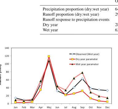
Dry year 28 30 Wet year 63 66 0 20 40 60 80 100 120 140

Ru

no

ff

(mm)

Observed (Wet year) Dry year parameter Wet year parameter

Figure 4.Quantification of predictive uncertainty in runoff simula-tions when the best parameter set (based on NS) calibrated for dry years was used for wet year observed series.

years was used for runoff prediction in wet years, runoff was underestimated by 35 % due to significant uncertainty that stemmed from the growing season months (Fig. 4). Mod-elling analysis also showed that no single metric can be an effective measure of model performance under dry and wet year conditions (Fig. 5a–c). However, utilizing a behavioural mean of these different performance metrics (Fig. 5d–f) ap-peared to be a more effective way of calibrating to extremely dry and wet hydroclimatic conditions. While the behavioural mean performed better in simulating runoff dynamics in win-ter through spring in the long-win-term record and significantly reduced the uncertainty in dry and wet years, larger uncer-tainty existed in summer through autumn months in dry and wet years compared to the long-term record.

3.5 Parameter uncertainty assessments

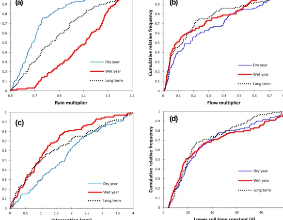
While we observed a wide prediction range from behavioural parameter sets (Fig. 5), we have limited information on the underlining processes. Therefore, we subjected the be-havioural parameter sets to further analysis to identify sen-sitive parameters and plausible patterns of hydrologic pro-cesses that differentiate dry and wet years (Fig. 6). The cu-mulative distribution function (CDF) of behavioural parame-ter sets showed that both rain and flow multipliers were sen-sitive parameters in dry years. The rain multiplier was less sensitive in wet years, unlike the flow multiplier. Long-term

simulations showed no sensitivity to the rain multiplier, but were sensitive to the flow multiplier. We observed similar patterns of response to the flow multiplier in all three hydro-logic regimes (Fig. 6b). The result also pointed to the sen-sitivity of interception in wet years, but all three hydrologic regimes showed similar patterns for the time constant (water residence time) in lower soil.

We subjected the pool of behavioural parameters in dry and wet year regimes to discriminant function analysis (DFA) to identify the key parameters that separate the ex-treme hydroclimatic conditions (Fig. 7). Results showed that both dry and wet years separated well in canonical space. However, the separation was driven mainly on quantitative parameters related to precipitation, interception and evapo-transpiration on canonical axis 1 (Rmult, Int and DDE). The parameters separated to a lesser extent on processes related to snow parameters on canonical axis 2 (Smult, SM and DDM). 3.6 Quantification of uncertainty in hydrologic

projections

We compared the effects of different performance metrics in wet and dry year regimes to constrain uncertainty in runoff projections under future hydroclimatic extremes in the Svart-berget catchment (Supplement Fig. 6). Results showed that differences in model representation of present-day conditions might be minimal (compared to the observed conditions), but a wide range of runoff regimes were projected in the future. We also observed a small difference in the range of runoff projections (derived from the minimum and maximum of behavioural parameter sets) using different model perfor-mance metrics. Uncertainties inherent in climate models (as opposed to differences in calibration or performance metrics) appeared to drive the overall uncertainty in runoff projections under dry and wet hydroclimatic conditions. The wet year is the closest to plausible projections of future conditions ex-pected in the boreal ecozone. However, model results sug-gested that the uncertainty in present-day long-term simula-tions is mostly driven by dry years. We compared the runoff predictions using dry year parameterization to parameteriza-tion based on wet years to quantify our current predictive uncertainty. Results showed that future runoff could be un-derpredicted by up to 40 % (relative to the wet year ensemble mean) if the projections are based on dry year

(8)

parameteriza-0 5 10 15 20 25 30 35 40 45

Ru no ff (mm)

Dry year

NS min NS max RMSE min RMSE max VAR min VAR max AD min AD max Observed 0 5 10 15 20 25 30 35 40 45

Ru no ff (mm)

Dry year

Observed Mean 0 20 40 60 80 100 120

Ru no ff (mm)

Wet year

NS min NS max RMSE min RMSE max VAR min VAR max AD min AD max Observed 0 20 40 60 80 100 120

Ru no ff (mm)

Wet year

Observed Mean 0 20 40 60 80 100 120

Ru no ff (mm)

Long term

Observed NS min NS max RMSE min RMSE max VAR min VAR max AD min AD max ₀ 20 40 60 80 100 120

Ru no ff (mm)

Long term

Observed Mean

(a)

(b)

( c )

(d)

(e)

(f)

Figure 5.Summary plots showing the prediction ranges of seasonal runoff dynamics of behavioural parameter sets using different

per-formance metrics in(a)dry years,(b)wet years and the(c)long term.(d)to(f)show the corresponding model performances using the

behavioural means of the metrics in(a)to(c).

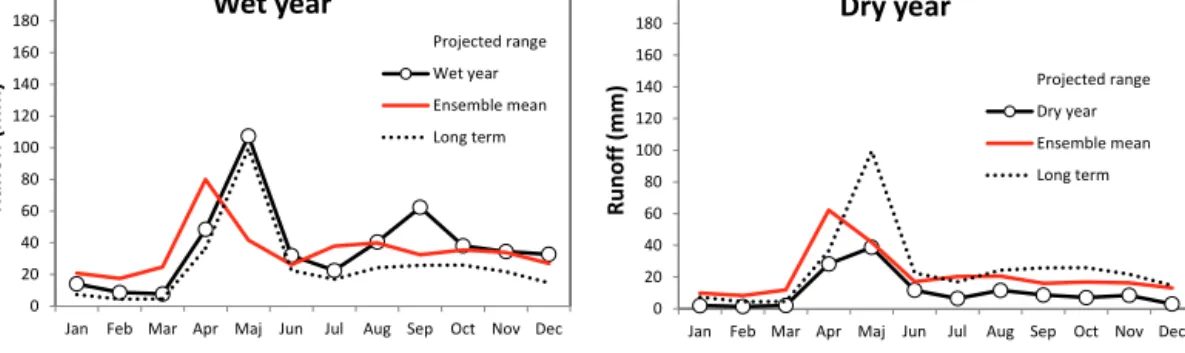
tion alone (Fig. 8). Both parameterizations projected a shift in spring melt from May to April in the future. However, en-semble projections showed that summer months could be a lot wetter (based on wet year parameterization compared to dry years) and the wet year spring peak could be up to 43 % more compared to projections based on the wet year ensem-ble mean.

4 Discussion

4.1 Insights from long-term hydroclimatic series Several studies have evaluated the impact of climate change on surface water resources (Berghuijs et al., 2014; Chou et al., 2013; Dore, 2005, among others), but most of these were

based on long-term series that depict mean system behaviour. However, present-day hydroclimatic extremes, such as those derived from historical wet and dry years, can be used as sim-ple proxies to gain insights that will aid our understanding of future hydroclimatic conditions. Using this approach we found that standard calibrations can result in underestimation of runoff by up to 35 % due to high variability of hydrocli-mate series in northern boreal catchments. Several explana-tions can be offered for the high variability in the long-term hydroclimate series at the study site. First, snowmelt hydrol-ogy is important in understanding the boreal water balances due to their location in the Northern Hemisphere (Euskirchen et al., 2007; Dore, 2005; Tetzlaff et al., 2011, 2013). As a re-sult, northern headwater catchments tend to show high vari-ability (Brown and Robinson, 2011; Burn, 2008).

(9)

0 0.1 0.2 0.3 0.4 0.5 0.6 0.7 0.8 0.9 1 0.5 0.7 0.9 1.1 1.3 1.5 Cu m ul at iv e r el at iv e fr eq uen cy Rain multiplier Dry year Wet year Long term 0 0.1 0.2 0.3 0.4 0.5 0.6 0.7 0.8 0.9 1 0 0.1 0.2 0.3 0.4 0.5 0.6 0.7 0.8 Cu m ul at iv e r el at iv e fr eq uen cy Flow multiplier Dry year Wet year Long term 0 0.1 0.2 0.3 0.4 0.5 0.6 0.7 0.8 0.9 1 0 0.5 1 1.5 2 2.5 3 3.5 4 Cu m ul at iv e r el at iv e fr eq uen cy Interception (mm) Dry year Wet year Long term 0 0.1 0.2 0.3 0.4 0.5 0.6 0.7 0.8 0.9 1 0 10 20 30 40 50 Cu m ul at iv e r el at iv e fr eq uen cy

Lower soil time constant (d)

Dry year Wet year Long term

(a) (b)

( c ) (d)

Figure 6.Cumulative distribution function (CDF) of behavioural parameters (top 100 iterations from the Monte Carlo runs) in wet and

dry years vs. the long-term record.(a)is the rain multiplier,(b)is the flow multiplier,(c)is the interception and(d)is the lower soil time

constant in the lower soil box. A rectangular distribution (straight line plot) defines parameter behaviours that were not sensitive (not left- or right-skewed).

Figure 7.Separation of the behavioural parameter sets (top 100 iter-ations from MCMC) in the dry and wet year hydrologic regimes us-ing discriminant function analysis (DFA). Wet and dry year hydrol-ogy separated mainly on parameters related to evapotranspiration (DDE), interception (Int) and rain multiplier (Rmult) on canonical 1. Parameters were separated on snow multiplier (Smult), snowmelt (SM) and degree day melt factor (DDM) on canonical 2. The circles represent normal 50 % contours. Parameters are defined in Table 3.

We observed annual runoff yield to be 63 % of total pre-cipitation in the wet years compared to 28 % of total precipi-tation in dry years. More runoff yield in the wet year regime could be seen as a result of near field capacity of the soils throughout the year, leading to greater propensity for runoff generation because hydrological conductivity increases to-wards the soil surface in the catchment (Nyberg et al., 2001). This can also imply more winter snow accumulation during the long winter period, resulting in higher spring melt that drives the overall water fluxes (Laudon et al., 2004). Less runoff yield in dry years could be attributed to higher soil moisture deficit and relatively more important evapotranspi-ration rates (Dai, 2013).

We also observed differences in dry/wet year peak sum-mer precipitation and a shift in the lowest precipitation in late winter/early spring. Despite the differences in precipi-tation, we observed similar patterns of runoff responses that only differ in terms of magnitude. This suggested that there was more effective rainfall (net available water) available to infiltrate, continuously recharge groundwater systems and generate runoff from upstream sources in wet years. Slightly warmer temperatures in summer months could drive more of

(10)

0 20 40 60 80 100 120 140 160 180 200

Ru no ff ( mm) Dry year Projected range Dry year Ensemble mean Long term 0 20 40 60 80 100 120 140 160 180 200

Ru no ff ( mm) Wet year Projected range Wet year Ensemble mean Long term

Figure 8.Example of the range of runoff projection using wet year parameterization that closely depicts the future vs. projected range based on dry year parameterization. The projected range was simulated to constrain uncertainty in extreme wet and dry conditions in the future

using the behavioural parameter sets (top 100 iterations from MCMC) for each of the 15 RCM scenarios (100 parameters by 15 RCMs=1500

runs each for dry and wet years). The ensemble mean represents the mean of the 1500 realizations, while long term depicts the mean of the long-term series.

growing season evapotranspiration in dry years. Small dif-ferences in temperature regime between wet and dry years, unlike precipitation, also explained why larger uncertainty and biases still exist during post-processing of precipitation series in using any scenario-based GCMs as observed in Sup-plement Fig. 2.

4.2 Multi-criteria calibration of hydrological models There has been considerable discussion about the calibrat-ing procedure in the hydrological modellcalibrat-ing community (An-dréassian et al., 2012; Booij and Krol, 2010; Efstratiadis and Koutsoyiannis, 2010; Oreskes et al., 1994; Price et al., 2012). One of the key reasons for this is the difference in goodness-of-fit measures utilized in each model (Krause et al., 2005; Pushpathala et al., 2012). The most common strategy is to calibrate hydrologic models using the NS statistic (Nash and Sutcliffe, 1970). However, many modellers believe that the NS-based method alone tends to underestimate variance in modelled time series as this metric could be biased toward high or low flow periods (Futter et al., 2014; Jain and Sud-heer, 2008; Pushpalatha et al., 2012; Willens, 2009). This promotes our use of multi-criteria statistics in model calibra-tions to constrain predictive uncertainty in hydrologic pro-jections to extreme dry and wet hydroclimatic conditions. Therefore, multi-criteria calibration objectives that assessed model performances using different goodness-of-fit metrics could aid our understanding of hydrologic behaviour in bo-real catchments. Our observation of differences in model performances in terms of NS and other metrics presented here is expected as a three box model proposed by Seib-ert and McDonnell (2002) similarly showed good fit for NS but poor fit using other metrics. However, none of these fo-cus on the extremes. Another way to evaluate a model for its performance in describing extremes is the approach pre-sented in Willems (2009) or the one by Van Steenberger and Willems (2012). However, lower model performance (based

on NS) for the long-term record is explainable as most hy-drologic models are based on mean system behaviour repre-sented by long-term rainfall–runoff processes (Futter et al., 2014; Oni et al., 2014b; Wellen et al., 2014).

The lower range of model performances in calibrating to the observed runoff in dry years is an indication of vari-able runoff generation processes associated with this wet-ness regime. Dry years cause drought-like conditions (Dai, 2011; Mishra and Singh, 2010) as a result of less water avail-ability that reduces hydrologic connectivity within the catch-ment. However, the model performed better when applied to wet and dry years individually compared to the long-term record based on NS statistics. This suggested that the mech-anisms driving hydrologic processes in dry and wet years might be similar, but their relative magnitude differs from long-term average conditions (Grayson et al., 1997). Better performance under dry conditions (compared to the average long term) can also be attributed to the bias of NS towards baseflow (Futter et al., 2014; Jain and Sudheer, 2008; Push-palatha et al., 2012). Durations of high flows associated with wet years are typically shorter than the low flow durations; as a result, higher flows receive lower weight because of the squared flow terms in the NS computation. Therefore the un-certainty is higher in extrapolating low flows (compared to high flows) and was also shown by others (Bae et al., 2011; Najafi et al., 2011; Maurer et al., 2010; Vansteenkiste et al., 2014b; Vélazquez et al., 2013).

However, NS statistics alone are not enough to assess model performances in climate-sensitive boreal headwater streams such as Svartberget. Other metrics such as the RMSE showed that dry years could be a major driver of the un-certainty we observed in simulating the long-term record. A possible explanation could be that the soil moisture deficit is larger in dry years, leading to soil matrix or vertical flow (Grayson et al., 1997) that can only generate runoff after fill-ing soil pore spaces (McDonnell, 1990). For example, soil pore spaces are usually not close to saturation under dry

(11)

con-ditions due to (1) intermittent precipitation events throughout the year and (2) several patchy source areas of high water convergence that are characterized by local landscape terrain or soil properties (Fang and Pomeroy, 2008; Jencso et al., 2009). Also, higher rates of evapotranspiration coupled with low precipitation can contribute to more spatially decoupled antecedent soil moisture conditions and thus lower runoff in dry years (Dai, 2013; Vicente-Serrano et al., 2010). There-fore, no single model performance metric can be effective in simulating the hydrology of dry and wet year conditions, as our results showed that the mean of behavioural metrics out-performed any individual metric in dry and wet years under present-day conditions.

4.3 Parameter sensitivity in dry and wet year regimes The robust uncertainty assessment conducted here showed that extensive exploration of model parameter spaces sug-gests how hydrologic behaviour differs between wet and dry year regimes. A possible explanation for the non-sensitivity of the rain multiplier in wet years could be attributed to (1) a more consistent or stable precipitation feeding the system throughout the year compared to intermittent precipitation in dry years (Fang and Pomeroy, 2008; McNamara et al., 2005) or (2) the effect of rainwater collector missing proportionally more rain in dry than wet years. This can explain the smaller spring peak that characterizes the dry year regime or its non-sensitivity to interception, unlike its role in wet year regimes. We observed that sensitivity of the lower soil time constant followed similar patterns in dry and wet years, unlike the up-per soil box. Therefore, we could expect a faster flow and higher runoff ratio in the wet years due to rapid response to precipitation events and more macropore flow (Peralta-Tapia et al., 2015). This can lead to steady runoff generation due to (1) near saturation of soils and (2) greater connectivity between stream channels and upland areas (Bracken et al., 2013; Ocampo et al., 2006) that become disconnected in dry years. The patterns of the flow multiplier parameter showed that both dry and wet year conditions followed similar runoff generation processes. These suggested that the main physi-cal mechanisms to explain parameter sensitivity and hydro-climatic behaviour to dry/wet conditions were related to dif-ferences in their precipitation patterns rather than landscape-driven hydrologic processes.

4.4 Drivers of hydrologic behaviour in dry and wet year regimes

Even though equifinality limits the use of CDFs alone in identifying all sensitive parameters, DFA of behavioural pa-rameters gave further holistic insights into plausible differ-ences in wet/dry hydrologic behaviour when projected on canonical space. This suggested that hydrological model pa-rameterizations calibrated to high flow associated with wet years differ from parameterizations for long-term or dry

con-ditions. Therefore, parameter separation primarily on quanti-tative parameters (Rmult, Int and DDE) related to rainfall and evapotranspiration on canonical axis 1 suggested that climate is still a first-order control of dry and wet year hydroclimatic regimes in the boreal forest. This is consistent with Wellen et al. (2014), who showed that extreme conditions could be triggered in a watershed when precipitation reaches a thresh-old that can initiate saturation overland flow. This is because soils are always near saturation capacity under prolonged wet conditions (Grayson et al., 1997). This can explain the in-crease in hydrologic model uncertainty in capturing the peak runoff events in wet years unless parameter ranges that com-bined different performance metrics are considered. Unfor-tunately, we might face a new challenge of increased precip-itation ranges in the future as climate changes (Chou et al., 2013; Dore, 2005). The separations of wet and dry years on snow process-related parameters (Smult, SM and DDM) and to a lesser extent on canonical axis 2 suggested that indirect landscape influences on snow processes could be important but are a second-order control on runoff response to dry and wet conditions. This agrees with Jencso et al. (2009), who showed that landscape mosaic structures with their unique source contribution areas control the overall watershed re-sponse.

4.5 Implications for future climate projections

Climate change in many places of the world leads to more extremes, both high and low flows. This study is not an ex-ception, as all 15 RCMs considered here projected a range of plausible futures in the Swedish boreal forest. Irrespective of the model performance metrics, results suggested that the future could be substantially wetter and could make drought conditions less severe in boreal ecozones. This could explain the large uncertainty in projecting runoff under wet condi-tions. For example, dry year and long-term parameterizations were similar and runoff was underpredicted by 35 % under the present-day condition when parameterization in dry years was used for wet years. This was due to large predictive un-certainty in runoff dynamics (Fig. 4) that resulted from high evapotranspiration rates during the snow-free growing sea-sons in dry years. This suggests that wet year calibration could give more credible projections of the future in the bo-real ecozone as the distribution of precipitation in wet years is closer to the precipitation pattern expected in the future. While our modelling results suggested negligible differences in runoff projections based on either dry year or long-term parameterization, wetter conditions could become a more dominant feature in the boreal ecozone.

These have implications for future climate change as both dry and wet year parametrization showed a consistent shift in spring melt patterns from May to April (Fig. 8). This temporal advance in spring melt patterns could result from altered distribution of snowfall and rainfall patterns in the winter (Berghuijs et al., 2014; Dore, 2005), and may likely

(12)

have effects on soil frost in the upper layer (Jungkvist et al., 2014) or change in evapotranspiration rates (Jung et al., 2010; Vicente-Serrano et al., 2010). Therefore, intensifica-tion of hydroclimatic regimes as climate changes in the fu-ture (Kunkel et al., 2013) could drive water quality issues to a new level in the boreal forest due to changes in the flux of organic carbon and aquatic pollutants. Furthermore, precip-itation has been shown to have much larger biogeochemical implications for the boreal carbon balance than previously anticipated (Öquist et al., 2014).

The large spread of mean annual runoff projected by each RCM in wet years is an indication of less agreement be-tween RCMs when predicting future conditions. This sug-gested that inherent uncertainty in climate models, rather than differences in model calibrations, drives the overall un-certainty in runoff projections. However, hydrologic model calibration for climate impact studies should be based on years that closely approximate anticipated conditions to bet-ter constrain uncertainty in projecting extremely dry and wet conditions in boreal and temperate regions.

The Supplement related to this article is available online at doi:10.5194/hess-20-2811-2016-supplement.

Acknowledgements. This project was funded by two larger

projects, ForWater and Future Forest, studying the effect of climate and forest management on boreal water resources. Funding for KCS came from the Swedish Science Council, Formas, SKB, MISTRA and the Kempe Foundation. The ENSEMBLES data used in this work were funded by EU FP6 Integrated Project EN-SEMBLES (contract number 505539), whose support is gratefully acknowledged. We also thank Patrick Willems of KU Leuven, Belgium and an anonymous reviewer for their insightful comments that greatly improved the manuscript.

Edited by: N. Verhoest

References

Andréassian, V., Le Moine, N., Perrin, C., Ramos, M. H., Oudin, L., Mathevet, T., Lerat, J., and Berthet, L.: All that glitters is not gold: the case of calibrating hydrological models, Hydrol. Process., 26, 2206–2210, 2012.

Andréassian, V., Bourgin, F., Oudin, L., Mathevet, T., Perrin, C., Lerat, J., Coron, L., and Berthet, L.: Seeking genericity in the selection of parameter sets: Impact on hydrological model effi-ciency, Water Resour. Res., 50, 8356–8366, 2014.

Bae, D. H., Jung, I. W., and Lettenmaier, D. P.: Hydrologic uncer-tainties in climate change from IPCC AR4 GCM simulations of the Chungju Basin, Korea, J. Hydrol., 401, 90–105, 2011. Berghuijs, W., Woods, R., and Hrachowitz, M.: A precipitation shift

from snow towards rain leads to a decrease in streamflow, Nature Clim. Change, 4, 583–586, 2014.

Beven, K.: A manifesto for the equifinality thesis, J. Hydrol., 320, 18–36, 2006.

Boe, J., Terray, L., Habets, F., and Martin, E.: Statistical and dynamical downscaling of the Seine basin climate for hydro-meteorological studies, Int. J. Climatol., 27, 1643–1655, doi:10.1002/joc.1602, 2007.

Bonan, G. B.: Forests and climate change: forcings, feedbacks, and the climate benefits of forests, Science, 320, 1444–1449, 2008. Booij, M. J. and Krol, M. S.: Balance between calibration objectives

in a conceptual hydrological model, Hydrol. Sci. J., 55, 1017– 1032, 2010.

Bosshard, T., Carambia, M., Goergen, K., Kotlarski, S., Krahe, P., Zappa, M., and Schär, C.: Quantifying uncertainty sources in an ensemble of hydrological climate-impact projections, Water Re-sour. Res., 49, 1523–1536, 2013.

Breuer, L., Huisman, J. A., Willems, P., Bormann, H., Bronstert, A., Croke, B. F. W., Frede, H. G., Gräff, T., Hubrechts, L., Jakeman, A. J., and Kite, G.: Assessing the impact of land use change on hydrology by ensemble modeling (LUCHEM). I: Model inter-comparison with current land use, Adv. Water Resour., 32, 129– 146, 2009.

Bracken, L., Wainwright, J., Ali, G., Tetzlaff, D., Smith, M., Re-aney, S., and Roy, A.: Concepts of hydrological connectivity: Research approaches, pathways and future agendas, Earth-Sci. Rev., 119, 17–34, 2013.

Brown, R. D. and Robinson, D. A.: Northern Hemisphere spring snow cover variability and change over 1922–2010 including an assessment of uncertainty, The Cryosphere, 5, 219–229, doi:10.5194/tc-5-219-2011, 2011.

Burn, D. H.: Climatic influences on streamflow timing in the head-waters of the Mackenzie River Basin, J. Hydrol., 352, 225–238, 2008.

Butts, M. B., Payne, J. T., Kristensen, M., and Madsen, H.: An eval-uation of the impact of model structure on hydrological mod-elling uncertainty for streamflow simulation, J. Hydrol., 298, 242–266, 2004.

Cao, W., Bowden, W. B., Davie, T., and Fenemor, A.: Multi-variable and multi-site calibration and validation of SWAT in a large mountainous catchment with high spatial variability, Hydrol. Process., 20, 1057–1073, 2006.

Chou, C., Chiang, J. C., Lan, C.-W., Chung, C.-H., Liao, Y.-C., and Lee, C.-J.: Increase in the range between wet and dry season pre-cipitation, Nature Geosci., 6, 263–267, 2013.

Coron, L., Andreassian, V., Perrin, C., Lerat, J., Vaze, J., Bourqui, M. and Hendrickx, F.: Crash testing hydrological models in con-trasted climate conditions: An experiment on 216 Australian catchments, Water Resour. Res., 48, W05552, 2012.

Dai, A.: Drought under global warming: a review, Wiley Interdisci-plinary Reviews: Climate Change, 2, 45–65, 2011.

Dai, A.: Increasing drought under global warming in observations and models, Nature Clim. Change, 3, 52–58, 2013.

Dore, M. H.: Climate change and changes in global precipitation patterns: what do we know?, Environ. Int., 31, 1167–1181, 2005. Donigian, A. S.: Watershed model calibration and validation: The HSPF experience, Proceedings of the Water Environment Feder-ation, 2002, 44–73, 2002.

Dosio, A. and Paruolo, P.: Bias correction of the ENSEMBLES high-resolution climate change projections for use by impact

(13)

models: Evaluation on the present climate, J. Geophys. Res.-Atmos., 116, D16106, 2011.

Efstratiadis, A. and Koutsoyiannis, D.: One decade of multi-objective calibration approaches in hydrological modelling: a re-view, Hydrol. Sci. J., 55, 58–78, 2010.

Ehret, U., Zehe, E., Wulfmeyer, V., Warrach-Sagi, K., and Liebert, J.: HESS Opinions “Should we apply bias correction to global and regional climate model data?,” Hydrol. Earth Syst. Sci., 16, 3391–3404, doi:10.5194/hess-16-3391-2012, 2012.

Euskirchen, E., McGuire, A., and Chapin, F. S.: Energy feedbacks of northern high-latitude ecosystems to the climate system due to reduced snow cover during 20th century warming, Global Change Biol., 13, 2425–2438, 2007.

Fang, X. and Pomeroy, J. W.: Drought impacts on Canadian prairie wetland snow hydrology, Hydrol. Process., 22, 2858–2873, 2008. Futter, M. N., Erlandsson, M. A., Butterfield, D., Whitehead, P. G., Oni, S. K., and Wade, A. J.: PERSiST: a flexible rainfall-runoff modelling toolkit for use with the INCA family of models, Hydrol. Earth Syst. Sci., 18, 855–873, doi:10.5194/hess-18-855-2014, 2014.

Grayson, R. B., Western, A. W., Chiew, F. H., and Blöschl, G.: Pre-ferred states in spatial soil moisture patterns: Local and nonlocal controls, Water Resour. Res., 33, 2897–2908, 1997.

Ines, A. V. M. and Hansen, J. W.: Bias correction of daily GCM rainfall for crop simulation studies, Agr. Forest Meteorol., 138, 44–53, doi:10.1016/j.agrformet.2006.03.009, 2006.

IPCC: The physical science basis. contribution of working group I to the fourth assessment report of the intergovernmental panel on climate change, in: Climate Change 2007: The Physical Sci-ence Basis, edited by: Solomon, S., Qin, D., Manning, M., Chen, Z., Marquis, M., Averyt, K. B., Tignor, M., and Miller, H. L., Cambridge University Press, Cambridge, UK and New York, NY, USA, 996 pp., 2007.

Jain, S. K. and Sudheer, K.: Fitting of hydrologic models: a close look at the Nash–Sutcliffe index, J. Hydrol. Eng., 13, 981–986, 2008.

Jencso, K. G., McGlynn, B. L., Gooseff, M. N., Wondzell, S. M., Bencala, K. E., and Marshall, L. A.: Hydrologic connectivity be-tween landscapes and streams: Transferring reach-and plot-scale understanding to the catchment scale, Water Resour. Res., 45, W04428, 2009.

Jung, M., Reichstein, M., Ciais, P., Seneviratne, S. I., Sheffield, J., Goulden, M. L., Bonan, G., Cescatti, A., Chen, J., and De Jeu, R.: Recent decline in the global land evapotranspiration trend due to limited moisture supply, Nature, 467, 951–954, 2010.

Jungqvist, G., Oni, S. K., Teutschbein, C., and Futter, M.

N.: Effect of climate change on soil temperature in

Swedish boreal forests, PLoS ONE, 10, 1371, e93957, doi:10.1371/journal.pone.0093957, 2014.

Karlsson, I. B., Sonnenborg, T. O., Jensen, K. H., and Refsgaard, J. C.: Historical trends in precipitation and stream discharge at the Skjern River catchment, Denmark, Hydrol. Earth Syst. Sci., 18, 595–610, doi:10.5194/hess-18-595-2014, 2014.

Klemeš, V.: Operational testing of hydrological simulation models, Hydrol. Sci. J., 31, 13–24, 1986.

Krause, P., Boyle, D., and Bäse, F.: Comparison of different effi-ciency criteria for hydrological model assessment, Adv. Geosci., 5, 89–97, 2005.

Kunkel, K. E., Karl, T. R., Easterling, D. R., Redmond, K., Young, J., Yin, X., and Hennon, P.: Probable maximum precipitation and climate change, Geophys. Res. Lett., 40, 1402–1408, 2013. Larssen, T., Høgåsen, T., and Cosby, B. J.: Impact of time series

data on calibration and prediction uncertainty for a deterministic hydrogeochemical model, Ecol. Model., 207, 22–33, 2007. Laudon, H. and Ottosson Löfvenius, M.: Adding snow to the

picture–providing complementary winter precipitation data to

the Krycklan catchment study database, Hydrol. Process.,Doi:

10.1002/hyp.10753, 2015.

Laudon, H., Seibert, J., Köhler, S., and Bishop, K.: Hydro-logical flow paths during snowmelt: Congruence between hydrometric measurements and oxygen 18 in meltwater, soil water, and runoff, Water Resour. Res., 40, W03102, doi:10.1029/2003WR002455, 2004.

Laudon, H., Taberman, I., Ågren, A., Futter, M., Ottosson-Löfvenius, M., and Bishop, K.: The Krycklan Catchment Study—a flagship infrastructure for hydrology, biogeochemistry, and climate research in the boreal landscape, Water Resour. Res., 49, 7154–7158, 2013.

Ledesma, J. L. J., Futter, M. N., Laudon, H., Evans, C. D., and Köhler, S. J: Boreal forest riparian zones regulate stream sul-fate and dissolved organic carbon, Sci. Total Environ., 560–561, 110–122, doi:10.1016/j.scitotenv.2016.03.230, 2016.

Li, H., Xu, C.-Y., and Beldring, S.: How much can we gain with increasing model complexity with the same model concepts?, J. Hydrol., 527, 858–871, 2015.

Lindner, M., Maroschek, M., Netherer, S., Kremer, A., Barbati, A., Garcia-Gonzalo, J., Seidl, R., Delzon, S., Corona, P., and Kol-ström, M.: Climate change impacts, adaptive capacity, and vul-nerability of European forest ecosystems, Forest Ecol. Manage., 259, 698–709, 2010.

Lindstrom, G., Pers, C., Rosberg, J., Stromqvist, J., and Arheimer, B.: Development and testing of the HYPE (Hydrological Pre-dictions for the Environment) water quality model for different spatial scales, Hydrol. Res., 41, 295–319, 2010.

Mascaro, G., Piras, M., Deidda, R. and Vivoni, E. R.: Distributed hydrologic modeling of a sparsely monitored basin in Sardinia, Italy, through hydrometeorological downscaling, Hydrology and Earth System Sciences, 17(10), 4143-4158, 2013.

Maurer, E. P., Brekke, L. D., and Pruitt, T.: Contrasting lumped and distributed hydrology models for estimating climate change im-pacts on California Watersheds, J. Am. Water Resour. Assoc., 4685, 1024–1035, 2010.

McDonnell, J. J.: A rationale for old water discharge through macropores in a steep, humid catchment, Water Resour. Res, 26, 2821–2832, 1990.

McNamara, J. P., Chandler, D., Seyfried, M., and Achet, S.: Soil moisture states, lateral flow, and streamflow generation in a semi-arid, snowmelt-driven catchment, Hydrol. Process., 19, 4023– 4038, 2005.

Mishra, A. K. and Singh, V. P.: A review of drought concepts, J. Hydrol., 391, 202–216, 2010.

Muerth, M. J., Gauvin St-Denis, B., Ricard, S., Velázquez, J. A., Schmid, J., Minville, M., Caya, D., Chaumont, D., Ludwig, R., and Turcotte, R.: On the need for bias correction in regional cli-mate scenarios to assess clicli-mate change impacts on river runoff, Hydrol. Earth Syst. Sci., 17, 1189–1204, doi:10.5194/hess-17-1189-2013, 2013.

(14)

Najafi, M. R., Moradkhani, H., and Jung, I. W.: Assessing the uncer-tainties of hydrologic model selection in climate change impact studies, Hydrol. Process., 25, 2814–2826, 2011.

Nash, J. E. and Sutcliffe, J.: River flow forecasting through concep-tual models part I—A discussion of principles, J. Hydrol., 10, 282–290, 1970.

Nyberg, L., Stähli, M., Mellander, P. E., and Bishop, K. H.: Soil frost effects on soil water and runoff dynamics along a boreal forest transect: 1. Field investigations, Hydrol. Process. 15, 909– 926, 2001.

Ocampo, C. J., Sivapalan, M., and Oldham, C.: Hydrological con-nectivity of upland-riparian zones in agricultural catchments: Im-plications for runoff generation and nitrate transport, J. Hydrol., 331, 643–658, 2006.

Oni, S. K., Futter, M. N., Bishop, K., Köhler, S. J., Ottosson-Löfvenius, M., and Laudon, H.: Long-term patterns in dis-solved organic carbon, major elements and trace metals in boreal headwater catchments: trends, mechanisms and heterogeneity, Biogeosciences, 10, 2315–2330, doi:10.5194/bg-10-2315-2013, 2013.

Oni, S., Futter, M., Teutschbein, C., and Laudon, H.: Cross-scale ensemble projections of dissolved organic carbon dynam-ics in boreal forest streams, Clim. Dynam., 42, 2305–2321, doi:10.1007/s00382-014-2124-6, 2014a.

Oni, S., Futter, M., Molot, L., Dillon, P., and Crossman, J.: Un-certainty assessments and hydrological implications of climate change in two adjacent agricultural catchments of a rapidly ur-banizing watershed, Sci. Total Environ., 473, 326–337, 2014b. Oni, S. K., Futter, M. N., Buttle, J., and Dillon, P. J.:

Hydrolog-ical footprints of urban developments in the Lake Simcoe wa-tershed, Canada: a combined paired-catchment and change de-tection modelling approach, Hydrol. Process., 29, 1829–1843, 2015a.

Oni, S. K., Tiwari, T., Ledesma, J. L., Ågren, A. M., Teutschbein, C., Schelker, J., Laudon, H., and Futter, M. N.: Local-and landscape-scale impacts of clear-cuts and climate change on sur-face water dissolved organic carbon in boreal forests, J. Geophys. Res.-Biogeosci., 120, 2402–2426, 2015b.

Oreskes, N., Shrader-Frechette, K., and Belitz, K.: Verification, val-idation, and confirmation of numerical models in the earth sci-ences, Science, 263, 641–646, 1994.

Öquist, M., Bishop, K., Grelle, A., Klemedtsson, L., Köhler, S., Laudon, H., Lindroth, A., Ottosson Löfvenius, M., Wallin, M. B., and Nilsson, M. B.: The full annual carbon balance of boreal forests is highly sensitive to precipitation, Environ. Sci. Technol. Lett., 1, 315–319, 2014.

Peralta-Tapia, A., Sponseller, R. A., Tetzlaff, D., Soulsby, C., and Laudon, H.: Connecting precipitation inputs and soil flow path-ways to stream water in contrasting boreal catchments, Hydrol. Process., 29, 3546–3555, 2015.

Porporato, A., Daly, E., and Rodriguez-Iturbe, I.: Soil water balance and ecosystem response to climate change, Am. Natural., 164, 625–632, 2004.

Price, K., Purucker, S. T., Kraemer, S. R., and Babendreier, J. E.: Tradeoffs among watershed model calibration targets for parameter estimation, Water Resour. Res., 48, W10542, doi:10.1029/2012WR012005, 2012.

Pushpalatha, R., Perrin, C., Le Moine, N., and Andréassian, V.: A review of efficiency criteria suitable for evaluating low-flow sim-ulations, J. Hydrol., 420, 171–182, 2012.

Räty, O., Räisänen, J., and Ylhäisi, J. S.: Evaluation of delta change and bias correction methods for future daily precipitation: in-termodel cross-validation using ENSEMBLES simulations, Cli-mate dynamics, 42, 2287–2303, 2014.

Refsgaard, J. C. and Knudsen, J.: Operational validation and inter-comparison of different types of hydrological models, Water Re-sour. Res., 32, 2189–2202, 1996.

Refsgaard, J. C., Van der Sluijs, J. P., Brown, J., and Van der Keur, P.: A framework for dealing with uncertainty due to model struc-ture error, Adv. Water Resour., 29, 1586-1597, 2006.

Refsgaard, J. C., Madsen, H., Andréassian, V., Arnbjerg-Nielsen, K., Davidson, T. A., Drews, M., Hamilton, D. P., Jeppesen, E., Kjellström, E., Olesen, J. E. and Sonnenborg, T. O.: A framework for testing the ability of models to project climate change and its impacts, Clim. Change, 122, 271–282, 2014.

Ren, D. and Henderson-Sellers, A.: An analytical hydrological model for the study of scaling issues in land surface modeling, Earth Interact., 10, 1–24, 2006.

Seibert, J. and McDonnell, J. J.: On the dialog between experimen-talist and modeler in catchment hydrology: Use of soft data for multicriteria model calibration, Water Resour. Res., 38, 23-21– 23-14, 2002.

Seibert, J.: Reliability of model predictions outside calibration con-ditions, Hydrol. Res., 34, 477–492, 2003.

Senatore, A., Mendicino, G., Smiatek, G., and Kunstmann, H.: Re-gional climate change projections and hydrological impact anal-ysis for a Mediterranean basin in Southern Italy, J. Hydrol., 399, 70–92, 2011.

Tetzlaff, D., McDonnell, J., Uhlenbrook, S., McGuire, K., Bogaart, P., Naef, F., Baird, A., Dunn, S., and Soulsby, C.: Conceptualiz-ing catchment processes: simply too complex?, Hydrol. Process., 22, 1727, doi:10.1002/hyp.7069, 2008.

Tetzlaff, D., Soulsby, C., Hrachowitz, M., and Speed, M.: Relative influence of upland and lowland headwaters on the isotope hy-drology and transit times of larger catchments, J. Hydrol., 400, 438–447, 2011.

Tetzlaff, D., Soulsby, C., Buttle, J., Capell, R., Carey, S., Laudon, H., McDonnell, J., McGuire, K., Seibert, S., and Shanley, J.: Catchments on the cusp? Structural and functional change in northern ecohydrology, Hydrol. Process., 27, 766–774, doi:10.1002/hyp.9700, 2013.

Teutschbein, C. and Seibert, J.: Bias correction of regional climate model simulations for hydrological climate-change impact stud-ies: Review and evaluation of different methods, J. Hydrol., 456– 457, 12–29, 2012.

Trenberth, K. E.: Framing the way to relate climate extremes to cli-mate change, Climatic Change, 115, 283–290, 2012.

Van der Linden, P. and Mitchell, J. F. B.: ENSEMBLE: Climate change and its impacts: Summary of research and results from the ENSEMBLES project: http://ensembles-eu.metoffice.com/ docs/Ensembles_final_report_Nov09.pdf, 2009.

Van Steenbergen, N. and Willems, P.: Method for testing the accu-racy of rainfall–runoff models in predicting peak flow changes due to rainfall changes, in a climate changing context, J. Hydrol., 414, 425–434, 2012.

(15)

Vansteenkiste, T., Tavakoli, M., Van Steenbergen, N., De Smedt, F., Batelaan, O., Pereira, F., and Willems, P.: Intercomparison of five lumped and distributed models for catchment runoff and extreme flow simulation, J. Hydrol., 511, 335–349, 2014a.

Vansteenkiste, T., Tavakoli, M., Ntegeka, V., De Smedt, F., Bate-laan, O., Pereira, F., and Willems, P.: Intercomparison of hydro-logical model structures and calibration approaches in climate scenario impact projections, J. Hydrol., 519, 743–755, 2014b. Velázquez, J. A., Schmid, J., Ricard, S., Muerth, M. J., Gauvin

St-Denis, B., Minville, M., Chaumont, D., Caya, D., Ludwig, R., and Turcotte, R.: An ensemble approach to assess hydrological models’ contribution to uncertainties in the analysis of climate change impact on water resources, Hydrology and Earth System Sciences, 17, 565–578, 2013.

Vicente-Serrano, S. M., Beguería, S., and López-Moreno, J. I.: A multiscalar drought index sensitive to global warming: the stan-dardized precipitation evapotranspiration index, J. Climate, 23, 1696–1718, 2010.

Vörösmarty, C. J., Green, P., Salisbury, J., and Lammers, R. B.: Global water resources: vulnerability from climate change and population growth, Science, 289, 284–288, 2000.

Wellen, C., Arhonditsis, G. B., Long, T., and Boyd, D.: Accommo-dating environmental thresholds and extreme events in hydrolog-ical models: a Bayesian approach, J. Great Lakes Res., 40, 102– 116, 2014.

Wilby, R. L.: Uncertainty in water resource model parameters used for climate change impact assessment, Hydrol. Process., 19, 3201–3219, 2005. Willems, P.: A time series tool to support the multi-criteria performance evaluation of rainfall-runoff models, Environ. Model. Softw., 24, 311–321, 2009.