A Tutorial on Machine Learning and Data Science Tools with Python

and Data Science Tools with Python

{marcus.bloice,andreas.holzinger}@medunigraz.at

Abstract. In this tutorial, we will provide an introduction to the main Python software tools used for applying machine learning techniques to medical data. The focus will be on open-source software that is freely available and is cross platform. To aid the learning experience, a com-panion GitHub repository is available so that you can follow the examples contained in this paper interactively using Jupyter notebooks. The note-books will be more exhaustive than what is contained in this chapter, and will focus on medical datasets and healthcare problems. Briefly, this tutorial will first introduce Python as a language, and then describe some of the lower level, general matrix and data structure packages that are popular in the machine learning and data science communities, such as NumPy and Pandas. From there, we will move to dedicated machine learning software, such as SciKit-Learn. Finally we will introduce the Keras deep learning and neural networks library. The emphasis of this paper is readability, with as little jargon used as possible. No previous experience with machine learning is assumed. We will use openly avail-able medical datasets throughout.

Keywords: Machine learning

·

·

·

Tools

·

·

1

Introduction

The target audience for this tutorial paper are those who wish to quickly get started in the area of data science and machine learning. We will provide an overview of the current and most popular libraries with a focus on Python, however we will mention alternatives in other languages where appropriate. All tools presented here are free and open source, and many are licensed under very flexible terms (including, for example, commercial use). Each library will be introduced, code will be shown, and typical use cases will be described. Medical datasets will be used to demonstrate several of the algorithms.

Machine learning itself is a fast growing technical field [1] and is highly rele-vant topic in both academia and in the industry. It is therefore a relerele-vant skill to have in both academia and in the private sector. It is a field at the intersection of informatics and statistics, tightly connected with data science and knowledge

c

Springer International Publishing AG 2016

A. Holzinger (Ed.): ML for Health Informatics, LNAI 9605, pp. 435–480, 2016. DOI: 10.1007/978-3-319-50478-0 22

discovery [2,3]. The prerequisites for this tutorial are therefore a basic under-standing of statistics, as well as some experience in any C-style language. Some knowledge of Python is useful but not a must.

An accompanying GitHub repository is provided to aid the tutorial: https://github.com/mdbloice/MLDS

It contains a number of notebooks, one for each main section. The notebooks will be referred to where relevant.

2

Glossary and Key Terms

This section provides a quick reference for several algorithms that are not explic-ity mentioned in this chapter, but may be of interest to the reader. This should provide the reader with some keywords or useful points of reference for other similar libraries to those discussed in this chapter.

BIDMach GPU accelerated machine learning library for algorithms that are not necessarily neural network based.

Caretprovides a standardised API for many of the most useful machine learn-ing packages for R. Seehttp://topepo.github.io/caret/index.html. For read-ers who are more comfortable with R, Caret provides a good substitute for Python’s SciKit-Learn.

Mathematica is a commercial symbolic mathematical computation system, developed since 1988 by Wolfram, Inc. It provides powerful machine learning techniques “out of the box” such as image classification [4].

MATLAB is short for MATrix LABoratory, which is a commercial numeri-cal computing environment, and is a proprietary programming language by MathWorks. It is very popular at universities where it is often licensed. It was originally built on the idea that most computing applications in some way rely on storage and manipulations of one fundamental object—the matrix, and this is still a popular approach [5].

Ris used extensively by the statistics community. The software package Caret provides a standardised API for many of R’s machine learning libraries.

WEKAis short for the Waikato Environment for Knowledge Analysis [6] and has been a very popular open source tool since its inception in 1993. In 2005 Weka received the SIGKDD Data Mining and Knowledge Discovery Service Award: it is easy to learn and simple to use, and provides a GUI to many machine learning algorithms [7].

Vowpal Wabbit Microsoft’s machine learning library. Mature and actively developed, with an emphasis on performance.

3

Requirements and Installation

The most convenient way of installing the Python requirements for this tutorial is by using the Anaconda scientific Python distribution. Anaconda is a collection

of the most commonly used Python packages preconfigured and ready to use. Approximately 150 scientific packages are included in the Anaconda installation.

To install Anaconda, visit

https://www.continuum.io/downloads

and install the version of Anaconda for your operating system.

All Python software described here is available for Windows, Linux, and Macintosh. All code samples presented in this tutorial were tested under Ubuntu Linux 14.04 using Python 2.7. Some code examples may not work on Windows without slight modification (e.g. file paths in Windows use \ and not / as in UNIX type systems).

The main software used in a typical Python machine learning pipeline can consist of almost any combination of the following tools:

1. NumPy, for matrix and vector manipulation

2. Pandas for time series and R-like DataFrame data structures 3. The 2D plotting library matplotlib

4. SciKit-Learn as a source for many machine learning algorithms and utilities 5. Keras for neural networks and deep learning

Each will be covered in this book chapter.

3.1 Managing Packages

Anaconda comes with its own built in package manager, known as Conda. Using the conda command from the terminal, you can download, update, and delete Python packages. Conda takes care of all dependencies and ensures that packages are preconfigured to work with all other packages you may have installed.

First, ensure you have installed Anaconda, as per the instructions under https://www.continuum.io/downloads.

Keeping your Python distribution up to date and well maintained is essential in this fast moving field. However, Anaconda makes it particularly easy to man-age and keep your scientific stack up to date. Once Anaconda is installed you can manage your Python distribution, and all the scientific packages installed by Anaconda using the conda application from the command line. To list all packages currently installed, useconda list. This will output all packages and their version numbers. Updating all Anaconda packages in your system is per-formed using the conda update -all command. Conda itself can be updated using the conda update condacommand, while Python can be updated using the conda update python command. To search for packages, use the search

parameter, e.g.conda search stats wherestatsis the name or partial name of the package you are searching for.

4

Interactive Development Environments

4.1 IPython

IPython is a REPL that is commonly used for Python development. It is included in the Anaconda distribution. To start IPython, run:

1 $ i p y t h o n

Listing 1.Starting IPython

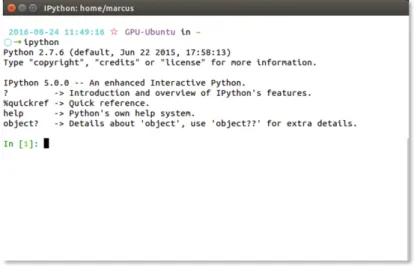
Some informational data will be displayed, similar to what is seen in Fig.1, and you will then be presented with a command prompt.

Fig. 1.The IPython Shell.

IPython is what is known as a REPL: a Read Evaluate Print Loop. The interpreter allows you to type in commands which are evaluated as soon as you press the Enter key. Any returned output is immediately shown in the console. For example, we may type the following:

1 In [1]: 1 + 1 2 Out [1]: 2 3 In [2]: i m p o r t math 4 In [3]: math . r a d i a n s (90) 5 Out [3]: 1 . 5 7 0 7 9 6 3 2 6 7 9 4 8 9 6 6 6 In [4]:

Listing 2.Examining the Read Evaluate Print Loop (REPL)

After pressing return (Line 1 in Listing2), Python immediately interprets the line and responds with the returned result (Line 2 in Listing2). The interpreter then awaits the next command, hence Read Evaluate Print Loop.

Using IPython to experiment with code allows you to test ideas without needing to create a file (e.g.fibonacci.py) and running this file from the com-mand line (by typing python fibonacci.py at the command prompt). Using the IPython REPL, this entire process can be made much easier. Of course, creating permanent files is essential for larger projects.

A useful feature of IPython are the so-called magic functions. These com-mands are not interpreted as Python code by the REPL, instead they are special commands that IPython understands. For example, to run a Python script you can use the%run magic function:

1 > > > % run f i b o n a c c i . py 30 2 F i b o n a c c i n u m b e r 30 is 8 3 2 0 4 0 .

Listing 3.Using the%runmagic function to execute a file.

In the code above, we have executed the Python code contained in the file

fibonacci.pyand passed the value 30 as an argument to the file.

The file is executed as a Python script, and its output is displayed in the shell. Other magic functions include%timeitfor timing code execution: 1 > > > def f i b o n a c c i ( n ) :

2 ... if n == 0: r e t u r n 0 3 ... if n == 1: r e t u r n 1

4 ... r e t u r n f i b o n a c c i ( n -1) + f i b o n a c c i ( n -2) 5 > > > % t i m e i t f i b o n a c c i (25)

6 10 loops , best of 3: 30.9 ms per loop

Listing 4. The %timeit magic function can be used to check execution times of functions or any other piece of code.

As can be seen, executing the fibonacci(25) function takes on average 30.9 ms. The%timeitmagic function is clever in how many loops it performs to create an average result, this can be as few as 1 loop or as many as 10 million loops.

Other useful magic functions include%lsfor listing files in the current work-ing directory, %cdfor printing or changing the current directory, and %cpaste

for pasting in longer pieces of code that span multiple lines. A full list of magic functions can be displayed using, unsurprisingly, a magic function: type%magic

to view all magic functions along with documentation for each one. A summary of useful magic functions is shown in Table1.

Last, you can use the ? operator to display in-line help at any time. For example, typing 1 > > > abs ? 2 D o c s t r i n g : 3 abs ( n u m b e r ) -> n u m b e r 4 5 R e t u r n the a b s o l u t e v a l u e of the a r g u m e n t . 6 Type : b u i l t i n _ f u n c t i o n _ o r _ m e t h o d

Listing 5.Accessing help within the IPython console.

For larger projects, or for projects that you may want to share, IPython may not be ideal. In Sect.4.2we discuss the web-based notebook IDE known as Jupyter, which is more suited to larger projects or projects you might want to share.

Table 1.A non-comprehensive list of IPython magic functions. Magic Command Description

%lsmagic Lists all the magic functions

%magic Shows descriptive magic function documentation

%ls Lists files in the current directory

%cd Shows or changes the current directory

%who Shows variables in scope

%whos Shows variables in scope along with type information %cpaste Pastes code that spans several lines

%reset Resets the session, removing all imports and deleting all variables %debug Starts a debuggerpost mortem

4.2 Jupyter

Jupyter, previously known as IPython Notebook, is a web-based, interac-tive development environment. Originally developed for Python, it has since expanded to support over 40 other programming languages including Julia and R.

Jupyter allows fornotebooksto be written that contain text, live code, images, and equations. These notebooks can be shared, and can even be hosted on GitHub for free.

For each section of this tutorial, you can download a Juypter notebook that allows you to edit and experiment with the code and examples for each topic. Jupyter is part of the Anaconda distribution, it can be started from the command line using using thejupytercommand:

1 $ j u p y t e r n o t e b o o k

Listing 6.Starting Jupyter

Upon typing this command the Jupyter server will start, and you will briefly see some information messages, including, for example, the URL and port at which the server is running (by default http://localhost:8888/). Once the server has started, it will then open your default browser and point it to this address. This browser window will display the contents of the directory where you ran the command.

To create a notebook and begin writing, click the New button and select Python. A new notebook will appear in a new tab in the browser. A Jupyter notebook allows you to run code blocks and immediately see the output of these blocks of code, much like the IPython REPL discussed in Sect.4.1.

Jupyter has a number of short-cuts to make navigating the notebook and entering code or text quickly and easily. For a list of short-cuts, use the menu Help→Keyboard Shortcuts.

4.3 Spyder

For larger projects, often a fully fledged IDE is more useful than Juypter’s notebook-based IDE. For such purposes, the Spyder IDE is often used. Spyder stands for Scientific PYthon Development EnviRonment, and is included in the Anaconda distribution. It can be started by typing spyder in the com-mand line.

5

Requirements and Conventions

This tutorial makes use of a number of packages which are used extensively in the Python machine learning community. In this chapter, the NumPy, Pandas, and Matplotlib are used throughout. Therefore, for the Python code samples shown in each section, we will presume that the following packages are available and have been loaded before each script is run:

1 > > > i m p o r t n u m p y as np 2 > > > i m p o r t p a n d a s as pd

3 > > > i m p o r t m a t p l o t l i b . p y p l o t as plt

Listing 7.Standard libraries used throughout this chapter. Throughout this chapter we will assume these libraries have been imported before each script.

Any further packages will be explicitly loaded in each code sample. However, in general you should probably follow each section’s Jupyter notebook as you are reading.

In Python code blocks, lines that begin with >>> represent Python code that should be entered into a Python interpreter (See Listing7 for an example). Output from any Python code is shownwithoutany preceding>>>characters. Commands which need to be entered into the terminal (e.g. bash or the MS-DOS command prompt) begin with$, such as:

1 $ l s −lAh

2 t o t a l 299K

3−rw−rw−r−− 1 b l o i c e admin 73K Sep 1 1 4 : 1 1 C l u s t e r i n g . ipynb

4−rw−rw−r−− 1 b l o i c e admin 57K Aug 25 1 6 : 0 4 Pandas . ipynb

5 . . .

Listing 8.Commands for the terminal are preceded by a$sign.

Output from the console is shownwithouta preceding$ sign. Some of the commands in this chapter may only work under Linux (such as the example usage of the lscommand in the code listing above, the equivalent in Windows is the

dir command). Most commands will, however, work under Linux, Macintosh, and Windows—if this is not the case, we will explicitly say so.

5.1 Data

For the Introduction to Python, NumPy, and Pandas sections we will work with either generated data or with a toy dataset. Later in the chapter, we will move

on to medical examples, including a breast cancer dataset, a diabetes dataset, and a high-dimensional gene expression dataset. All medical datasets used in this chapter are freely available and we will describe how to get the data in each relevant section. In earlier sections, generated data will suffice in order to demonstrate example usage, while later we will see that analysing more involved medical data using the same open-source tools is equally possible.

6

Introduction to Python

Python is a general purpose programming language that is used for anything from web-development to deep learning. According to several metrics, it is ranked as one of the top three most popular languages. It is now the most frequently taught introductory language at top U.S. universities according to a recent ACM blog article [8]. Due to its popularity, Python has a thriving open source commu-nity, and there are over 80,000 free software packages available for the language on the official Python Package Index (PyPI).

In this section we will give a very short crash course on using Python. These code samples will work best with a Python REPL interpreter, such as IPython or Jupyter (Sects.4.1and 4.2respectively). In the code below we introduce the some simple arithmetic syntax:

1 > > > 2 + 6 + (8 * 9) 2 80 3 > > > 3 / 2 4 1 5 > > > 3.0 / 2 6 1.5 7 > > > 4 ** 4 # To the p o w e r of 8 256

Listing 9.Simple arithmetic with Python in the IPython shell.

Python is a dynamically typed language, so you do not define the type of variable you are creating, it is inferred:

1 > > > n = 5 2 > > > f = 5.5 3 > > > s =" 5 " 4 > > > type ( s ) 5 str 6 > > > type ( f ) 7 f l o a t 8 > > > " 5 " * 5 9 " 5 5 5 5 5 " 10 > > > int (" 5 ") * 5 11 25

You can check types using the built-in type function. Python does away with much of the verbosity of languages such as Java, you do not even need to surround code blocks with brackets or braces:

1 > > > if " 5 " == 5:

2 ... p r i n t(" Will not get here ") 3 > > > elif int (" 5 ") == 5:

4 ... p r i n t(" Got here ") 5 Got here

Listing 11.Statement blocks in Python are indicated using indentation. As you can see, we use indentation to define our statement blocks. This is the number one source of confusion among those new to Python, so it is important you are aware of it. Also, whereas assignment uses=, we check equality using==(and inversely!=). Control of flow is handled byif,elif,while,for, and so on.

While there are several basic data structures, here we will concentrate on lists and dictionaries (we will cover much more on data structures in Sect.7.1). Other types of data structures are, for example, tuples, which are immutable—their contents cannot be changed after they are created—and sets, where repetition is not permitted. We will not cover tuples or sets in this tutorial chapter, however. Below we first define a list and then perform a number of operations on this list: 1 > > > p o w e r s = [1 , 2 , 4 , 8 , 16 , 32] 2 > > > p o w e r s 3 [1 , 2 , 4 , 8 , 16 , 32] 4 > > > p o w e r s [0] 5 1 6 > > > p o w e r s . a p p e n d ( 6 4 ) 7 > > > p o w e r s 8 [1 , 2 , 4 , 8 , 16 , 32 , 64] 9 > > > p o w e r s . i n s e r t (0 , 0) 10 > > > p o w e r s 11 [0 , 1 , 2 , 4 , 8 , 16 , 32 , 64] 12 > > > del p o w e r s [0] 13 > > > p o w e r s 14 [1 , 2 , 4 , 8 , 16 , 32 , 64] 15 > > > 1 in p o w e r s 16 True 17 > > > 100 not in p o w e r s 18 True

Listing 12.Operations on lists.

Lists are defined using square [] brackets. You can index a list using its numerical, zero-based index, as seen on Line 4. Adding values is performed using theappend andinsertfunctions. Theinsert function allows you to define in which position you would like the item to be inserted—on Line 9 of Listing12 we insert the number 0 at position 0. On Lines 15 and 17, you can see how we can use theinkeyword to check for membership.

You just saw that lists are indexed using zero-based numbering, we will now introduce dictionaries which are key-based. Data in dictionaries are stored using key-value pairs, and are indexed by the keys that you define:

1 > > > n u m b e r s = {" b i n g o ": 3458080 , " t u p p y ": 3 4 5 9 0 9 0 } 2 > > > n u m b e r s 3 {" b i n g o ": 3458080 , " t u p p y ": 3 4 5 9 0 9 0 } 4 > > > n u m b e r s [" b i n g o "] 5 3 4 5 8 0 8 0 6 > > > n u m b e r s [" m o n t y "] = 3 4 5 6 0 6 0 7 > > > n u m b e r s 8 {" b i n g o ": 3458080 , " m o n t y ": 3456060 , " t u p p y ": 3 4 5 9 0 9 0 } 9 > > > " t u p p y " in n u m b e r s 10 True

Listing 13.Dictionaries in Python.

We use curly{}braces to define dictionaries, and we must define both their values and their indices (Line 1). We can access elements of a dictionary using their keys, as in Line 4. On Line 6 we insert a new key-value pair. Notice that dictionaries are not ordered. On Line 9 we can also use theinkeyword to check for membership.

To traverse through a dictionary, we use aforstatement in conjunction with a function depending on what data we wish to access from the dictionary:

1 > > > for name , n u m b e r in n u m b e r s . i t e r i t e m s () : 2 ... p r i n t(" Name : " + name + " , n u m b e r : " + str ( n u m b e r ) ) 3 Name : bingo , n u m b e r : 3 4 5 8 0 8 0 4 Name : monty , n u m b e r : 3 4 5 6 0 6 0 5 Name : tuppy , n u m b e r : 3 4 5 9 0 9 0 6

7 > > > for key in n u m b e r s . keys () : 8 ... p r i n t( key ) 9 b i n g o 10 m o n t y 11 t u p p y 12 13 > > > for val in n u m b e r s . v a l u e s () : 14 ... p r i n t( val ) 15 3 4 5 8 0 8 0 16 3 4 5 6 0 6 0 17 3 4 5 9 0 9 0

Listing 14.Iterating through dictionaries.

First, the code above traverses through each key-value pair using

iteritems() (Line 1). When doing so, you can specify a variable name for each key and value (in that order). In other words, on Line 1, we have stated that we wish to store each key in the variable nameand each value in the vari-ablenumber as we go through theforloop. You can also access only the keys or values using thekeysandvaluesfunctions respectively (Lines 7 and 13).

As mentioned previously, many packages are available for Python. These need to be loaded into the current environment before they are used. For example, the code below uses theosmodule, which we must first import before using:

1 > > > i m p o r t os 2 > > > os . l i s t d i r (" ./ ") 3 [" B o o k C h a p t e r . i p y n b ", 4 " N u m P y . i p y n b ", 5 " P a n d a s . i p y n b ", 6 " f i b o n a c c i . py ", 7 " L i n e a r R e g r e s s i o n . i p y n b ", 8 " C l u s t e r i n g . i p y n b "] 9 > > > from os i m p o r t l i s t d i r # A l t e r n a t i v e l y 10 > > > l i s t d i r (" ./ ") 11 [" B o o k C h a p t e r . i p y n b ", 12 " N u m P y . i p y n b ", 13 ...

Listing 15.Importing packages using theimportkeyword.

Two ways of importing are shown here. On Line 1 we are importing the entire

os name space. This means we need to call functions using theos.listdir()

syntax. If you know that you only need one function or submodule you can import it individually using the method shown on Line 9. This is often the preferred method of importing in Python.

Lastly, we will briefly see how functions are defined using thedefkeyword: 1 > > > def a d d N u m b e r s ( x , y ) :

2 ... r e t u r n x + y 3 > > > a d d N u m b e r s (4 , 2) 4 6

Listing 16.Functions are defined using thedefkeyword.

Notice that you do not need to define the return type, or the arguments’ types. Classes are equally easy to define, and this is done using the class key-word. We will not cover classes in this tutorial. Classes are generally arranged into modules, and further into packages. Now that we have covered some of the basics of Python, we will move on to more advanced data structures such as 2-dimensional arrays and data frames.

7

Handling Data

7.1 Data Structures and Notation

In machine learning, more often than not the data that you analyse will be stored in matrices and vectors. Generally speaking, your data that you wish to analyse will be stored in the form of a matrix, often denoted using a bold upper case symbol, generallyX, and your label data will be stored in a vector, denoted with a lower case bold symbol, ofteny.

A data matrixXwithnsamples andmfeatures is denoted as follows: X∈Rn×m= ⎡ ⎢ ⎢ ⎢ ⎢ ⎢ ⎣ x1,1 x1,2 x1,3 . . . x1,m x2,1 x2,2 x2,3 . . . x2,m x3,1 x3,2 x3,3 . . . x3,m .. . ... ... . .. ... x_n,1xn,2xn,3. . . xn,m ⎤ ⎥ ⎥ ⎥ ⎥ ⎥ ⎦

Each column,m, of this matrix contains the features of your data and each row,n, is a sample of your data. A single sample of your data is denoted by its subscript, e.g.x_i= [x_i,1xi,2xi,3 · · · xi,m]

In supervised learning, your labels or targets are stored in a vector:

y∈Rn×1= ⎡ ⎢ ⎢ ⎢ ⎢ ⎢ ⎣ y1 y2 y3 .. . y_n ⎤ ⎥ ⎥ ⎥ ⎥ ⎥ ⎦

Note that number of elements in the vector y is equal to the number of samplesnin your data matrixX, hencey∈Rn×1_.

For a concrete example, let us look at the famous Iris dataset. The Iris flower dataset is a small toy dataset consisting ofn= 150samples or observations of three species of Iris flower (Iris setosa, Iris virginica, and Iris versicolor). Each sample, or row, has m = 4 features, which are measurements relating to that sample, such as the petal length and petal width. Therefore, the features of the Iris dataset correspond to the columns in Table2, namely sepal length, sepal width, petal length, and petal width. Each observation or sample corresponds to one row in the table. Table2shows a few rows of the Iris dataset so that you can become acquainted with how it is structured. As we will be using this dataset in several sections of this chapter, take a few moments to examine it.

Table 2.The Iris flower dataset.

Sepal length Sepal width Petal length Petal width Class

1 5.1 3.5 1.4 0.2 setosa 2 4.9 3.0 1.4 0.2 setosa 3 4.7 3.2 1.3 0.2 setosa .. . ... ... ... ... ... 150 5.9 3.0 5.1 1.8 virginica

In a machine learning task, you would store this table in a matrixX, where

with 150 rows and 4 columns (generally we will store such data in a variable named X). The 1st _{row in Table2 corresponds to 1}st _{row of X, namely x}

1 = [5.1 3.5 1.4 0.2]. See Listing17 for how to represent a vector as an array and a matrix as a two-dimensional array in Python. While the data is stored in a matrixX, the Class column in Table2, which represents the species of plant, is stored separately in a target vectory. This vector contains what are known as the

targets orlabels of your dataset. In the Iris dataset,y= [y1y2 · · · y150], yi∈ {setosa, versicolor, virginica}. The labels can either be nominal, as is the case in the Iris dataset, or continuous. In a supervised machine learning problem, the principle aim is to predict the label for a given sample. If the targets are nominal, this is a classification problem. If the targets are continuous this is a regression problem. In an unsupervised machine learning task you do not have the target vector y, and you only have access to the datasetX. In such a scenario, the aim is to find patterns in the dataset X and cluster observations together, for example.

We will see examples of both classification algorithms and regression algo-rithms in this chapter as well as supervised and unsupervised problems.

1 > > > v1 = [5.1 , 3.5 , 1.4 , 0.2] 2 > > > v2 = [

3 ... [5.1 , 3.5 , 1.4 , 0.2] , 4 ... [4.9 , 3.0 , 1.3 , 0.2]

5 .. ]

Listing 17. Creating 1-dimensional (v1) and 2-dimensional data structures (v2) in Python (Note that in Python these are called lists).

In situations where your data is split into subsets, such as a training set and a test set, you will see notation such asXtrainandXtest. Datasets are often split into a training set and a test set, where the training set is used to learn a model, and the test set is used to check how well the model fits to unseen data.

In a machine learning task, you will almost always be using a library known as NumPy to handle vectors and matrices. NumPy provides very use-ful matrix manipulation and data structure functionality and is optimised for speed. NumPy is the de facto standard for data input, storage, and output in the Python machine learning and data science community1_{. Another important} library which is frequently used is the Pandas library for time series and tabular data structures. These packages compliment each other, and are often used side by side in a typical data science stack. We will learn the basics of NumPy and Pandas in this chapter, starting with NumPy in Sect.7.2.

1 _{To speed up certain numerical operations, the numexprand bottleneckoptimised}

libraries for Python can be installed. These are included in the Anaconda distribu-tion, readers who are not using Anaconda are recommended to install them both.

7.2 NumPy

NumPy is a general data structures, linear algebra, and matrix manipulation library for Python. Its syntax, and how it handles data structures and matrices is comparable to that of MATLAB2.

To use NumPy, first import it (the convention is to import it asnp, to avoid having to type outnumpyeach time):

1 > > > i m p o r t n u m p y as np

Listing 18.Importing NumPy. It is convention to import NumPy asnp. Rather than repeat this line for each code listing, we will assume you have imported NumPy, as per the instructions in Sect.3. Any further imports that may be required for a code sample will be explicitly mentioned.

Listing19 describes some basic usage of NumPy by first creating a NumPy array and then retrieving some of the elements of this array using a technique calledarray slicing:

1 > > > v e c t o r = np . a r a n g e ( 1 0 ) # M a k e an a r r a y f r o m 0 - 9 2 > > > v e c t o r 3 [0 , 1 , 2 , 3 , 4 , 5 , 6 , 7 , 8 , 9] 4 > > > v e c t o r [1] 5 1 6 > > > v e c t o r [ 0 : 3 ] 7 [0 , 1 , 2] 8 > > > v e c t o r [0: -3] # E l e m e n t 0 to the 3 rd last e l e m e n t 9 [0 , 1 , 2 , 3 , 4 , 5 , 6] 10 > > > v e c t o r [ 3 : 7 ] # F r o m i n d e x 3 but not i n c l u d i n g 7 11 [3 , 4 , 5 , 6]

Listing 19.Array slicing in NumPy.

In Listing19, Line 1 we have created a vector (actually a NumPy array) with 10 elements from 0–9. On Line 2 we simply print the contents of the vector, the contents of which are shown on Line 3. Arrays in Python are 0-indexed, that means to retrieve the first element you must use the number 0. On Line 4 we retrieve the 2nd element which is 1, using the square bracket index-ing syntax: array[i], where i is the index of the value you wish to retrieve fromarray. To retrieve subsets of arrays we use a method known asarray slic-ing, a powerful technique that you will use constantly, so it is worthwhile to study its usage carefully! For example, on Line 9 we are retrieving all elements beginning with element 0 to the 3rd last element. Slicing 1D arrays takes the form array[<startpos>:<endpos>], where the start position<startpos> and end position<endpos>are separated with a:character. Line 11 shows another example of array slicing. Array slicing includes the element indexed by the

<startpos> up to butnot includingthe element indexed by<endpos>.

2 _{Users of MATLAB may want to view this excellent guide to NumPy for MATLAB}

A very similar syntax is used for indexing 2-dimensional arrays, but now we must index first the rows we wish to retrieve followed by the columns we wish to retrieve. Some examples are shown below:

1 > > > m = np . a r a n g e (9) . r e s h a p e (3 ,3) 2 > > > m 3 a r r a y ([[0 , 1 , 2] , 4 [3 , 4 , 5] , 5 [6 , 7 , 8]]) 6 > > > m [0] # Row 0 7 a r r a y ([0 , 1 , 2]) 8 > > > m [0 , 1] # Row 0 , c o l u m n 1 9 1 10 > > > m [: , 0] # All rows , 0 th c o l u m n 11 a r r a y ([0 , 3 , 6])

12 > > > m [: ,:] # All rows , all c o l u m n s 13 a r r a y ([[0 , 1 , 2] , 14 [3 , 4 , 5] , 15 [6 , 7 , 8]]) 16 > > > m [ -2: , -2:] # L o w e r r i g h t c o r n e r of m a t r i x 17 a r r a y ([[4 , 5] , 18 [7 , 8]]) 19 > > > m [:2 , :2] # U p p e r l e f t c o r n e r of m a t r i x 20 a r r a y ([[0 , 1] , 21 [3 , 4]])

Listing 20.2D array slicing.

As can be seen, indexing 2-dimensional arrays is very similar to the 1-dimensional arrays shown previously. In the case of 2-dimensional arrays, you first specify your row indices, follow this with a comma (,) and then specify your column indices. These indices can be ranges, as with 1-dimensional arrays. See Fig.2 for a graphical representation of a number of array slicing operations in NumPy.

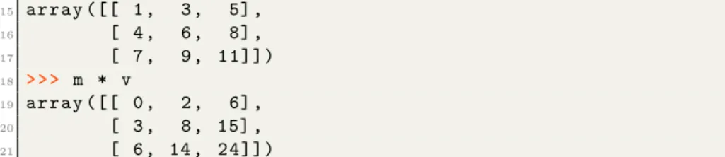
With element wise operations, you can apply an operation (very efficiently) to every element of ann-dimensional array:

1 > > > m + 1 2 a r r a y ([[1 , 2 , 3] , 3 [4 , 5 , 6] , 4 [7 , 8 , 9]]) 5 > > > m **2 # S q u a r e e v e r y e l e m e n t 6 a r r a y ([[ 0 , 1 , 4] , 7 [ 9 , 16 , 25] , 8 [36 , 49 , 6 4 ] ] ) 9 > > > v * 10 10 a r r a y ([ 10 , 20 , 30 , 40 , 50 , 60 , 70 , 80 , 90 , 1 0 0 ] ) 11 > > > v = np . a r r a y ([1 , 2 , 3]) 12 > > > v 13 a r r a y ([1 , 2 , 3]) 14 > > > m + v

15 a r r a y ([[ 1 , 3 , 5] , 16 [ 4 , 6 , 8] , 17 [ 7 , 9 , 1 1 ] ] ) 18 > > > m * v 19 a r r a y ([[ 0 , 2 , 6] , 20 [ 3 , 8 , 15] , 21 [ 6 , 14 , 2 4 ] ] )

Listing 21.Element wise operations and array broadcasting.

Fig. 2. Array slicing and indexing with NumPy. Image has been redrawn from the

original athttp://www.scipy-lectures.org/ images/numpy indexing.png.

There are a number of things happening in Listing21 that you should be aware of. First, in Line 1, you will see that if you apply an operation on a matrix or array, the operation will be appliedelement wise to each item in the

n-dimensional array. What happens when you try to apply an operation using, let’s say a vector and a matrix? On lines 14 and 18 we do exactly this. This is known asarray broadcasting, and works when two data structures share at least one dimension size. In this case we have a 3×3 matrix and are performing an operation using a vector with 3 elements.

7.3 Pandas

Pandas is a software library for data analysis of tabular and time series data. In many ways it reproduces the functionality of R’s DataFrame object. Also, many common features of Microsoft Excel can be performed using Pandas, such as “group by”, table pivots, and easy column deletion and insertion.

Pandas’ DataFrame objects are label-based (as opposed to index-based as is the case with NumPy), so that each column is typically given a name which can be called to perform operations. DataFrame objects are more similar to

spreadsheets, and each column of a DataFrame can have a different type, such as boolean, numeric, or text. Often, it should be stressed, you will use NumPy and Pandas in conjunction. The two libraries complement each other and are not competing frameworks, although there is overlap in functionality between the two. First, we must get some data. The Python package SciKit-Learn provides some sample data that we can use (we will learn more about SciKit-Learn later). SciKit-Learn is part of the standard Anaconda distribution.

In this example, we will load some sample data into a Pandas DataFrame object, then rename the DataFrame object’s columns, and lastly take a look at the first three rows contained in the DataFrame:

1 > > > i m p o r t p a n d a s as pd # C o n v e n t i o n 2 > > > from s k l e a r n i m p o r t d a t a s e t s 3 > > > iris = d a t a s e t s . l o a d _ i r i s () 4 > > > df = pd . D a t a F r a m e ( iris . data ) 5 > > > df . c o l u m n s = [" s e p a l _ l ", " s e p a l _ w ", " p e t a l _ l ", " p e t a l _ w "] 6 > > > df . head (3) 7 s e p a l _ l s e p a l _ w p e t a l _ l p e t a l _ w 8 0 5.1 3.5 1.4 0.2 9 1 4.9 3.0 1.4 0.2 10 2 4.7 3.2 1.3 0.2

Listing 22.Reading data into a Pandas DataFrame.

Selecting columns can performed using square brackets or dot notation: 1 > > > df [" s e p a l _ l "] 2 0 5.1 3 1 4.9 4 2 4.7 5 ... 6 > > > df . s e p a l _ l # A l t e r n a t i v e l y 7 0 5.1 8 1 4.9 9 2 4.7 10 ...

Listing 23.Accessing columns using Pandas’ syntax. You can use square brackets to access individual cells of a column: 1 > > > df [" s e p a l _ l "][0]

2 5.1

3 > > > df . s e p a l _ l [0] # A l t e r n a t i v e l y 4 5.1

To insert a column, for example the species of the plant, we can use the following syntax:

1 > > > df [" name "] = i r i s . t a r g e t

2 > > > df . loc [ df . name == 0 , " name "] = " s e t o s a " 3 > > > df . loc [ df . name == 1 , " name "] = " v e r s i c o l o r " 4 > > > df . loc [ df . name == 2 , " name "] = " v i r g i n i c a " 5 # A l t e r n a t i v e l y

6 > > > df [" name "] = [ iris . t a r g e t _ n a m e s [ x ] for x in iris . t a r g e t ]

Listing 25. Inserting a new column into a DataFrame and replacing its numerical values with text.

In Listing25above, we created a new column in our DataFrame calledname. This is a numerical class label, where 0 corresponds to setosa, 1 corresponds to versicolor, and 2 corresponds to virginica. First, we add the new column on Line 1, and we then replace these numerical values with text, shown in Lines 2–4. Alternatively, we could have just done this in one go, as shown on Line 6 (this uses a more advanced technique called a list comprehension).

We use thelocand iloc keywords for selecting rows and columns, in this case the 0th _row:

1 > > > df . iloc [0] 2 s e p a l _ l 5.1 3 s e p a l _ w 3.5 4 p e t a l _ l 1.4 5 p e t a l _ w 0.2 6 n a m e s e t o s a 7 N a m e : 0 , d t y p e : o b j e c t

Listing 26. Theilocfunction is used to access items within a DataFrame by their index rather than their label.

You use loc for selecting with labels, and iloc for selecting with indices. Usingloc, we first specify the rows, then the columns, in this case we want the first three rows of the sepal lcolumn:

1 > > > df . loc [:3 , " s e p a l _ l "]

2 0 5.1

3 1 4.9

4 2 4.7

5 3 4.6

6 Name : sepal_l , dtype : f l o a t 6 4

Listing 27.Using thelocfunction also allows for more advanced commands. Because we are selecting a column using a label, we use the loc keyword above. Here we select the first 5 rows of the DataFrame usingiloc:

1 > > > df . iloc [:5] 2 s e p a l _ l s e p a l _ w p e t a l _ l p e t a l _ w name 3 0 5.1 3.5 1.4 0.2 s e t o s a 4 1 4.9 3.0 1.4 0.2 s e t o s a 5 2 4.7 3.2 1.3 0.2 s e t o s a 6 3 4.6 3.1 1.5 0.2 s e t o s a 7 4 5.0 3.6 1.4 0.2 s e t o s a 8 5 5.4 3.9 1.7 0.4 s e t o s a

Listing 28. Selecting the first 5 rows of the DataFrame using theiloc function. To

select items using text labels you must use thelockeyword.

Or rows 15 to 20 and columns 2 to 4: 1 > > > df . iloc [15:21 , 2:5] 2 p e t a l _ l p e t a l _ w name 3 15 1.5 0.4 s e t o s a 4 16 1.3 0.4 s e t o s a 5 17 1.4 0.3 s e t o s a 6 18 1.7 0.3 s e t o s a 7 19 1.5 0.3 s e t o s a 8 20 1.7 0.2 s e t o s a

Listing 29.Selecting specific rows and columns. This is done in much the same way as NumPy.

Now, we may want to quickly examine the DataFrame to view some of its properties: 1 > > > df . d e s c r i b e () 2 s e p a l _ l s e p a l _ w p e t a l _ l p e t a l _ w 3 c o u n t 1 5 0 . 0 0 0 0 0 0 1 5 0 . 0 0 0 0 0 0 1 5 0 . 0 0 0 0 0 0 1 5 0 . 0 0 0 0 0 0 4 mean 5 . 8 4 3 3 3 3 3 . 0 5 4 0 0 0 3 . 7 5 8 6 6 7 1 . 1 9 8 6 6 7 5 std 0 . 8 2 8 0 6 6 0 . 4 3 3 5 9 4 1 . 7 6 4 4 2 0 0 . 7 6 3 1 6 1 6 min 4 . 3 0 0 0 0 0 2 . 0 0 0 0 0 0 1 . 0 0 0 0 0 0 0 . 1 0 0 0 0 0 7 25% 5 . 1 0 0 0 0 0 2 . 8 0 0 0 0 0 1 . 6 0 0 0 0 0 0 . 3 0 0 0 0 0 8 50% 5 . 8 0 0 0 0 0 3 . 0 0 0 0 0 0 4 . 3 5 0 0 0 0 1 . 3 0 0 0 0 0 9 75% 6 . 4 0 0 0 0 0 3 . 3 0 0 0 0 0 5 . 1 0 0 0 0 0 1 . 8 0 0 0 0 0 10 max 7 . 9 0 0 0 0 0 4 . 4 0 0 0 0 0 6 . 9 0 0 0 0 0 2 . 5 0 0 0 0 0 Listing 30.Thedescribefunction prints some commonly required statistics regarding the DataFrame.

You will notice that thenamecolumn is not included as Pandas quietly ignores this column due to the fact that the column’s data cannot be analysed in the same way.

Sorting is performed using the sort values function: here we sort by the sepal length, named sepal lin the DataFrame:

1 > > > df . s o r t _ v a l u e s ( by =" s e p a l _ l ", a s c e n d i n g = True ) . head (5) 2 s e p a l _ l s e p a l _ w p e t a l _ l p e t a l _ w name 3 13 4.3 3.0 1.1 0.1 s e t o s a 4 42 4.4 3.2 1.3 0.2 s e t o s a 5 38 4.4 3.0 1.3 0.2 s e t o s a 6 8 4.4 2.9 1.4 0.2 s e t o s a 7 41 4.5 2.3 1.3 0.3 s e t o s a

Listing 31.Sorting a DataFrame using thesort valuesfunction.

A very powerful feature of Pandas is the ability to write conditions within the square brackets:

1 > > > df [ df . s e p a l _ l > 7] 2 s e p a l _ l s e p a l _ w p e t a l _ l p e t a l _ w name 3 102 7.1 3.0 5.9 2.1 v i r g i n i c a 4 105 7.6 3.0 6.6 2.1 v i r g i n i c a 5 107 7.3 2.9 6.3 1.8 v i r g i n i c a 6 109 7.2 3.6 6.1 2.5 v i r g i n i c a 7 117 7.7 3.8 6.7 2.2 v i r g i n i c a 8 118 7.7 2.6 6.9 2.3 v i r g i n i c a 9 122 7.7 2.8 6.7 2.0 v i r g i n i c a 10 125 7.2 3.2 6.0 1.8 v i r g i n i c a 11 129 7.2 3.0 5.8 1.6 v i r g i n i c a 12 130 7.4 2.8 6.1 1.9 v i r g i n i c a 13 131 7.9 3.8 6.4 2.0 v i r g i n i c a 14 135 7.7 3.0 6.1 2.3 v i r g i n i c a

Listing 32.Using a condition to select a subset of the data can be performed quickly using Pandas.

New columns can be easily inserted or removed (we saw an example of a column being inserted in Listing25, above):

1 > > > s e p a l _ l _ w = df . s e p a l _ l + df . s e p a l _ w 2 > > > df [" s e p a l _ l _ w "] = s e p a l _ l _ w # C r e a t e s a new c o l u m n 3 > > > df . head (5) 4 s e p a l _ l s e p a l _ w p e t a l _ l p e t a l _ w name s e p a l _ l _ w 5 0 5.1 3.5 1.4 0.2 s e t o s a 8.6 6 1 4.9 3.0 1.4 0.2 s e t o s a 7.9 7 2 4.7 3.2 1.3 0.2 s e t o s a 7.9 8 3 4.6 3.1 1.5 0.2 s e t o s a 7.7 9 4 5.0 3.6 1.4 0.2 s e t o s a 8.6

Listing 33.Adding and removing columns

There are few things to note here. On Line 1 of Listing33 we use the dot notation to access the DataFrame’s columns, however we could also have said

sepal l w = df["sepal l"] + df["sepal w"] to access the data in each col-umn. The next important thing to notice is that you can insert a new column easily by specifying a label that is new, as in Line 2 of Listing33. You can delete a column using thedelkeyword, as indel df["sepal l w"].

Missing data is often a problem in real world datasets. Here we will remove all cells where the value is greater than 7, replacing them with NaN (Not a Number): 1 > > > i m p o r t n u m p y as np 2 > > > len ( df ) 3 150 4 > > > df [ df > 7] = np . NaN 5 > > > df = df . d r o p n a ( how =" any ") 6 > > > len ( df ) 7 138

Listing 34.Dropping rows that contain missing data.

After replacing all values greater than 7 with NaN (Line 4), we used the

dropna function (Line 5) to remove the 12 rows with missing values. Alter-natively you may want to replace NaN values with a value with the fillna

function, for example the mean value for that column: 1 > > > for col in df . c o l u m n s :

2 ... df [ col ] = df [ col ]. f i l l n a ( v a l u e = df [ col ]. m e a n () ) Listing 35.Replacing missing data with mean values.

As if often the case with Pandas, there are several ways to do everything, and we could have used either of the following:

1 > > > df . f i l l n a (l a m b d a x : x . f i l l n a ( v a l u e = x . m e a n () ) 2 > > > df . f i l l n a ( df . m e a n () )

Listing 36.Demonstrating several ways to handle missing data.

Line 1 demonstrates the use of a lambda function: these are functions which are not declared and are a powerful feature of Python. Either of the above examples in Listing36are preferred to the loop shown in Listing35. Pandas offers a number of methods for handling missing data, including advanced interpolation techniques3.

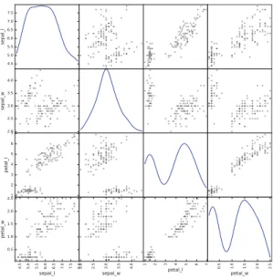
Plotting in Pandas uses matplotlib (more on which later), where publication quality prints can be created, for example you can quickly create a scatter matrix, a frequently used plot in data exploration to find correlations:

1 > > > from p a n d a s . t o o l s . p l o t t i n g i m p o r t s c a t t e r _ m a t r i x 2 > > > s c a t t e r _ m a t r i x ( df , d i a g o n a l =" kde ")

Listing 37.Several plotting features are built in to Pandas including scatter matrix functionality as shown here.

Which results in the scatter matrix seen in Fig.3. You can see that Pan-das is intelligent enough not to attempt to print the name column—these are known as nuisance columns and are silently, and temporarily, dropped for cer-tain operations. The kdeparameter specifies that you would like density plots 3 _{See http://pandas.pydata.org/pandas-docs/stable/missing data.html for more}

Fig. 3.Scatter matrix visualisation for the Iris dataset.

for the diagonal axis of the matrix, alternatively you can specify hist to plot histograms.

For many examples on how to use Pandas, refer to the SciPy Lectures website underhttp://www.scipy-lectures.org/. Much more on plotting and visualisation in Pandas can be found in the Pandas documentation, under: http://pandas. pydata.org/pandas-docs/stable/visualization.html. Last, a highly recommend-able book on the topic of Pandas and NumPy is Python for Data Analysis by Wes McKinney [9].

Now that we have covered an introduction into Pandas, we move on to visu-alisation and plotting using matplotlib and Seaborn.

8

Data Visualisation and Plotting

In Python, a commonly used 2D plotting library is matplotlib. It produces pub-lication quality plots, an example of which can be seen in Fig.4, which is created as follows:

1 > > > i m p o r t m a t p l o t l i b . p y p l o t as plt # C o n v e n t i o n 2 > > > x = np . r a n d o m . r a n d i n t (100 , size =25)

3 > > > y = x * x

4 > > > plt . s c a t t e r ( x , y ) ; plt . show ()

Listing 38.Plotting with matplotlib

This tutorial will not cover matplotlib in detail. We will, however, mention the Seaborn project, which is a high level abstraction of matplotlib, and has the added advantage that is creates better looking plots by default. Often all that is

Fig. 4.A scatter plot using matplotlib.

necessary is to import Seaborn, and plot as normal using matplotlib in order to profit from these superior looking plots. As well as better looking default plots, Seaborn has a number of very useful APIs to aid commonly performed tasks, such asfactorplot,pairplot, andjointgrid.

Seaborn can also perform quick analyses on the data itself. Listing39shows the same data being plotted, where a linear regression model is also fit by default:

1 > > > i m p o r t s e a b o r n as sns # C o n v e n t i o n 2 > > > sns . set () # Set d e f a u l t s 3 > > > x = np . r a n d o m . r a n d i n t (100 , size =25) 4 > > > y = x * x 5 > > > df = pd . D a t a F r a m e ({" x ": x , " y ": y }) 6 > > > sns . l m p l o t ( x =" x ", y =" y ", data = df ) ; plt . show () Listing 39.Plotting with Seaborn.

This will output a scatter plot but also will fit a linear regression model to the data, as seen in Fig.5.

For plotting and data exploration, Seaborn is a useful addition to the data scientist’s toolbox. However, matplotlib is more often than not the library you will encounter in tutorials, books, and blogs, and is the basis for libraries such as Seaborn. Therefore, knowing how to use both is recommended.

9

Machine Learning

We will now move on to the task of machine learning itself. In the following sec-tions we will describe how to use some basic algorithms, and perform regression, classification, and clustering on some freely available medical datasets concerning breast cancer and diabetes, and we will also take a look at a DNA microarrray dataset.

Fig. 5.Seaborn’slmplotfunction will fit a line to your data, which is useful for quick data exploration.

9.1 SciKit-Learn

SciKit-Learn provides a standardised interface to many of the most commonly used machine learning algorithms, and is the most popular and frequently used library for machine learning for Python. As well as providing many learning algorithms, SciKit-Learn has a large number of convenience functions for com-mon preprocessing tasks (for example, normalisation ork-fold cross validation). SciKit-Learn is a very large software library. For tutorials covering nearly all aspects of its usage seehttp://scikit-learn.org/stable/documentation.html. Sev-eral tutorials in this chapter followed the structure of examples found on the SciKit-Learn documentation website [10].

9.2 Linear Regression

In this example we will use a diabetes dataset that is available from SciKit-Learn’sdatasetspackage.

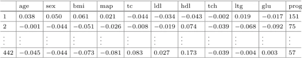
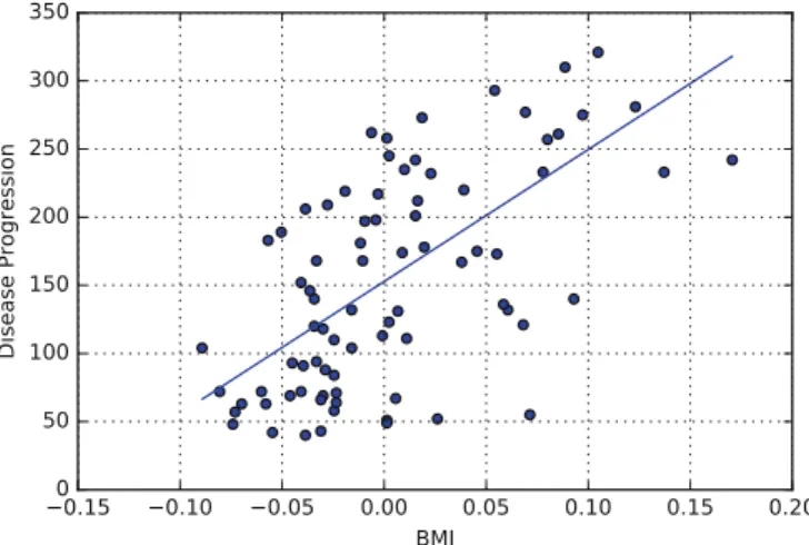
The diabetes dataset consists of 442 samples (the patients) each with 10 features. The features are the patient’s age, sex, body mass index (BMI), average blood pressure, and six blood serum values. The target is the disease progression. We wish to investigate if we can fit a linear model that can accurately predict the disease progression of a new patient given their data.

For visualisation purposes, however, we shall only take one of the features of the dataset, namely the Body Mass Index (BMI). So we shall investigate if there is correlation between BMI and disease progression (bmi and prog in Table3).

Table 3.Diabetes dataset

age sex bmi map tc ldl hdl tch ltg glu prog

1 0.038 0.050 0.061 0.021 −0.044 −0.034 −0.043 −0.002 0.019 −0.017 151 2 −0.001 −0.044 −0.051 −0.026 −0.008 −0.019 0.074 −0.039 −0.068 −0.092 75 . . . . . . . . . . . . . . . . . . . . . . . . . . . . . . . . . . . . 442 −0.045 −0.044 −0.073 −0.081 0.083 0.027 0.173 −0.039 −0.004 0.003 57 1 > > > from s k l e a r n i m p o r t datasets , l i n e a r _ m o d e l 2 > > > d = d a t a s e t s . l o a d _ d i a b e t e s () 3 > > > X = d . data 4 > > > y = d . t a r g e t 5 > > > np . s h a p e ( X ) 6 (442 , 10) 7 > > > X = X [: ,2] # T a k e o n l y the BMI c o l u m n ( i n d e x 2) 8 > > > X = X . r e s h a p e ( -1 , 1) 9 > > > y = y . r e s h a p e ( -1 , 1) 10 > > > np . s h a p e ( X ) 11 (442 , 1)

12 > > > X _ t r a i n = X [: -80] # We will use 80 s a m p l e s for t e s t i n g 13 > > > y _ t r a i n = y [: -80]

14 > > > X _ t e s t = X [ -80:] 15 > > > y _ t e s t = y [ -80:]

Listing 40.Loading a diabetes dataset and preparing it for analysis. Note once again that it is convention to store your target in a variable called

y and your data in a matrix called X (see Sect.7.1 for more details). In the example above, we first load the data in Lines 2–4, we then extract only the 3rd _{column, discarding the remaining 9 columns. Also, we split the data into a} training set, Xtrain, shown in the code as X trainand a test set,Xtest, shown in the code as X test. We did the same for the target vectory. Now that the data is prepared, we can train a linear regression model on the training data:

1 > > > l i n e a r _ r e g = l i n e a r _ m o d e l . L i n e a r R e g r e s s i o n () 2 > > > l i n e a r _ r e g . fit ( X_train , y _ t r a i n ) 3 L i n e a r R e g r e s s i o n ( c o p y _ X = True , f i t _ i n t e r c e p t = True , n _ j o b s =1 , n o r m a l i z e = F a l s e ) 4 > > > l i n e a r _ r e g . s c o r e ( X_test , y _ t e s t ) 5 0 . 3 6 4 6 9 9 1 0 6 9 6 1 6 3 7 6 5

Listing 41.Fitting a linear regression model to the data.

As we can see, after fitting the model to the training data (Lines 1–2), we test the trained model on the test set (Line 4). Plotting the data is done as follows:

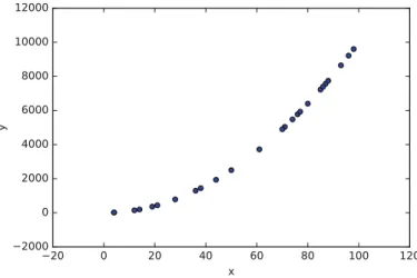
1 > > > plt . s c a t t e r ( X_test , y _ t e s t )

2 > > > plt . plot ( X_test , l i n e a r _ r e g . p r e d i c t ( X _ t e s t ) ) 3 > > > plt . show ()

Fig. 6.A model generated by linear regression showing a possible correlation between Body Mass Index and diabetes disease progression.

A similar output to that shown in Fig.6 will appear.

Because we wished to visualise the correlation in 2D, we extracted only one feature from the dataset, namely the Body Mass Index feature. However, there is no reason why we need to remove features in order to plot possible correla-tions. In the next example we will use Ridge regression on the diabetes dataset maintaining 9 from 10 of its features (we will discard the gender feature for simplicity as it is a nominal value). First let us split the data and apply it to a Ridge regression algorithm:

1 > > > from s k l e a r n i m p o r t c r o s s _ v a l i d a t i o n 2 > > > from s k l e a r n . p r e p r o c e s s i n g i m p o r t n o r m a l i z e 3 > > > X = d a t a s e t s . l o a d _ d i a b e t e s () . data 4 > > > y = d a t a s e t s . l o a d _ d i a b e t e s () . t a r g e t 5 > > > y = np . r e s h a p e ( y , ( -1 ,1) ) 6 > > > X = np . d e l e t e ( X , 1 , 1) # r e m o v e col 1 , a x i s 1

7 > > > X_train , X_test , y_train , y _ t e s t = c r o s s _ v a l i d a t i o n . t r a i n _ t e s t _ s p l i t ( X , y , t e s t _ s i z e = 0 . 2 )

Listing 43.Preparing a cross validation dataset.

We now have a shuffled train and test split using the cross validation

function (previously we simply used the last 80 observations inXas a test set, which can be problematic—proper shuffling of your dataset before creating a train/test split is almost always a good idea).

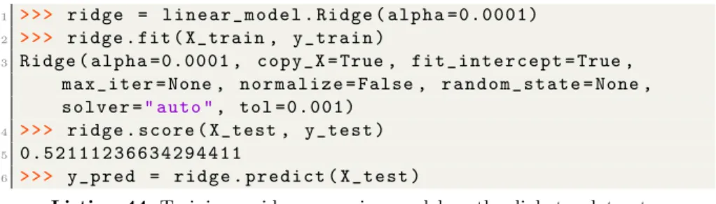
Now that we have preprocessed the data correctly, and have our train/test splits, we can train a model on the training setX train:

1 > > > r i d g e = l i n e a r _ m o d e l . R i d g e ( a l p h a = 0 . 0 0 0 1 ) 2 > > > ridge . fit ( X_train , y _ t r a i n )

3 R i d g e ( a l p h a = 0 . 0 0 0 1 , c o p y _ X = True , f i t _ i n t e r c e p t = True , m a x _ i t e r = None , n o r m a l i z e = False , r a n d o m _ s t a t e = None , s o l v e r =" auto ", tol = 0 . 0 0 1 )

4 > > > r i d g e . s c o r e ( X_test , y _ t e s t ) 5 0 . 5 2 1 1 1 2 3 6 6 3 4 2 9 4 4 1 1

6 > > > y _ p r e d = r i d g e . p r e d i c t ( X _ t e s t )

Listing 44.Training a ridge regression model on the diabetes dataset. We have made out predictions, but how do we plot our results? The linear regression model was built on 9-dimensional data set, so what exactly should we plot? The answer is to plot the predicted outcome versus the actual outcome for the test set, and see if this follows any kind of a linear trend. We do this as follows:

1 > > > plt . s c a t t e r ( y_test , y _ p r e d )

2 > > > plt . plot ([ y . min () , y . max () ] , [ y . min () , y . max () ]) Listing 45.Plotting the predicted versus the actual values. The resulting plot can be see in Fig.7.

Fig. 7.Plotting the predicted versus the actual values in the test set, using a model trained on a separate training set.

However, you may have noticed a slight problem here: if we had taken a dif-ferent test/train split, we would have gotten different results. Hence it is common to perform a 10-fold cross validation:

1 > > > from s k l e a r n . c r o s s _ v a l i d a t i o n i m p o r t c r o s s _ v a l _ s c o r e , c r o s s _ v a l _ p r e d i c t 2 > > > r i d g e _ c v = l i n e a r _ m o d e l . R i d g e ( a l p h a = 0 . 1 ) 3 > > > s c o r e _ c v = c r o s s _ v a l _ s c o r e ( ridge_cv , X , y , cv =10) 4 > > > s c o r e _ c v . mean () 5 0 . 4 5 3 5 8 7 2 8 0 3 2 6 3 4 4 9 9 6 > > > y_cv = c r o s s _ v a l _ p r e d i c t ( ridge_cv , X , y , cv =10) 7 > > > plt . s c a t t e r ( y , y_cv )

8 > > > plt . plot ([ y . min () , y . max () ] , [ y . min () , y . max () ]) ; Listing 46.Computing the cross validated score.

The results of the 10-fold cross validated scored can see in Fig.8.

Fig. 8.Plotting predictions versus the actual values using cross validation.

9.3 Non-linear Regression and Model Complexity

Many relationships between two variables are not linear, and SciKit-Learn has several algorithms for non-linear regression. One such algorithm is the Support Vector Regression algorithm, or SVR. SVR allows you to learn several types of models using different kernels. Linear models can be learned with a linear kernel, while non-linear curves can be learned using a polynomial kernel (where you can specify the degree) for example. As well as this, SVR in SciKit Learn can use a Radial Basis Function, Sigmoid function, or your own custom kernel.

For example, the code below will produce similar data to the examples shown in Sect.8.

1 > > > x = np . r a n d o m . r a n d ( 1 0 0 ) 2 > > > y = x * x 3 > > > y [ : : 5 ] += 0.4 # add 0.4 to e v e r y 5 th i t e m 4 > > > x . sort () 5 > > > y . sort () 6 > > > plt . s c a t t e r ( x , y ) ; plot . show () ;

Listing 47. Creating a non-smooth curve dataset for demonstration of various regression techniques.

This will produce data similar to what is seen in Fig.9. The data describes an almost linear relationship between xand y. We added some noise to this in Line 3 of Listing47.

Fig. 9.The generated dataset which we will fit our regression models to.

Now we will fit a function to this data using an SVR with a linear kernel. The code for this is as follows:

1 > > > lin = l i n e a r _ m o d e l . L i n e a r R e g r e s s i o n () 2 > > > x = x . r e s h a p e ( -1 , 1) 3 > > > y = y . r e s h a p e ( -1 , 1) 4 > > > lin . fit ( x , y ) 5 L i n e a r R e g r e s s i o n ( c o p y _ X = True , f i t _ i n t e r c e p t = True , n _ j o b s =1 , n o r m a l i z e = F a l s e ) 6 > > > lin . fit ( x , y ) 7 > > > lin . s c o r e ( x , y ) 8 0 . 9 2 2 2 2 0 2 5 3 7 4 7 1 0 5 5 9

Listing 48.Training a linear regression model on the generated non-linear data. We will now plot the result of the fitted model over the data, to see for ourselves how well the line fits the data:

1 > > > plt . s c a t t e r ( x , y , l a b e l =" Data ") 2 > > > plt . p l o t ( x , lin . p r e d i c t ( x ) ) 3 > > > plot . show ()

Listing 49.Plotting the linear model’s predictions. The result of this code can be seen in Fig.10.

Fig. 10.Linear regression on a demonstration dataset.

While this does fit the data quite well, we can do better—but not with a linear function. To achieve a better fit, we will now use a non-linear regression model, an SVR with a polynomial kernel of degree 3. The code to fit a polynomial SVR is as follows: 1 > > > from s k l e a r n . svm i m p o r t SVR 2 > > > p o l y _ s v m = SVR ( k e r n e l =" poly ", C = 1 0 0 0 ) 3 > > > p o l y _ s v m . fit ( x , y ) 4 SVR ( C =1000 , c a c h e _ s i z e =200 , c o e f 0 =0.0 , d e g r e e =3 , e p s i l o n =0.1 , g a m m a =" auto ", k e r n e l =" poly ", m a x _ i t e r = -1 , s h r i n k i n g = True , tol =0.001 , v e r b o s e = F a l s e ) 5 > > > p o l y _ s v m . s c o r e ( x , y ) 6 0 . 9 4 2 7 3 3 2 9 5 8 0 4 4 7 3 1 8

Listing 50.Training a polynomial Support Vector Regression model. Notice that the SciKit-Learn API exposes common interfaces irregardless of the model—both the linear regression algorithm and the support vector regres-sion algorithm are trained in exactly the same way, i.e.: they take the same basic parameters and expect the same data types and formats (Xandy) as input. This makes experimentation with many different algorithms easy. Also, notice that once you have called the fit() function in both cases (Listings48 and 50),

a summary of the model’s parameters are returned. These do, of course, vary from algorithm to algorithm.

You can see the results of this fit in Fig.11, the code to produce this plot is as follows:

1 > > > plt . s c a t t e r ( x , y , l a b e l =" Data ") 2 > > > plt . p l o t ( x , p o l y _ s v m . p r e d i c t ( x ) )

Listing 51. Plotting the results of the Support Vector Regression model with polynomial kernel.

Now we will use an Radial Basis Function Kernel. This should be able to fit the data even better:

Fig. 11.Fitting a Support Vector Regression algorithm with a polynomial kernel to a sample dataset. 1 > > > r b f _ s v m = SVR ( k e r n e l =" rbf ", C = 1 0 0 0 ) 2 > > > r b f _ s v m . fit ( x , y ) 3 SVR ( C =1000 , c a c h e _ s i z e =200 , c o e f 0 =0.0 , d e g r e e =3 , e p s i l o n =0.1 , g a m m a =’ auto ’, k e r n e l =’ rbf ’, m a x _ i t e r = -1 , s h r i n k i n g = True , tol =0.001 , v e r b o s e = F a l s e ) 4 > > > r b f _ s v m . s c o r e ( x , y ) 5 0 . 9 5 5 8 3 2 2 9 4 0 9 9 3 6 0 8 8

Listing 52.Training a Support Vector Regression model with a Radial Basis Function (RBF) kernel.

The result of this fit can be plotted: 1 > > > plt . s c a t t e r ( x , y , l a b e l =" Data ") 2 > > > plt . p l o t ( x , r b f _ s v m . p r e d i c t ( x ) )

Fig. 12. Non-linear regression using a Support Vector Regression algorithm with a Radial Basis Function kernel.

The plot can be seen in Fig.12. You will notice that this model probably fits the data best.

A Note on Model Complexity. It should be pointed out that a more complex model willalmost alwaysfit data better than a simpler model given the same dataset. As you increase the complexity of a polynomial by adding terms, you eventually will have as many terms as data points and you will fit the data perfectly, even fitting to outliers. In other words, a polynomial of, say, degree 4 will nearly always fit the same data better than a polynomial of degree 3— however, this also means that the more complex model could be fitting to noise. Once a model has begun to overfit it is no longer useful as a predictor to new data. There are various methods to spot overfitting, the most commonly used methods are to split your data into a training set and a test set and a method called cross validation. The simplest method is to perform a train/test split: we split the data into a training set and a test set—we then train our model on the training set but we subsequently measure the loss of the model on the held-back test set. This loss can be used to compare different models of different complexity. The best performing model will be that which minimises the loss on the test set.

Cross validation involves splitting the dataset in a way that each data sample is used once for training and for testing. In 2-fold cross validation, the data is shuffled and split into two equal parts: one half of the data is then used for training your model and the other half is used to test your model—this is then reversed, where the original test set is used to train the model and the original training set is used to test the newly created model. The performance is measured averaged across the test set splits. However, more often than not you will find that k-fold cross validation is used in machine learning, where, let’s say, 10%

of the data is held back for testing, while the algorithm is trained on 90% of the data, and this is repeated 10 times in a stratified manner in order to get the average result (this would be 10-fold cross validation). We saw how SciKit-Learn can perform a 10-fold cross validation simply in Sect.9.2.

9.4 Clustering

Clustering algorithms focus on ordering data together into groups. In general clustering algorithms are unsupervised—they require no y response variable as input. That is to say, they attempt to find groups or clusters within data where you do not know the label for each sample. SciKit-Learn has many clustering algorithms, but in this section we will demonstrate hierarchical clustering on a DNA expression microarray dataset using an algorithm from the SciPy library. We will plot a visualisation of the clustering using what is known as a dendro-gram, also using the SciPy library.

In this example, we will use a dataset that is described in Sect. 14.3 of the Elements of Statistical Learning [11]. The microarray data are available from the book’s companion website. The data comprises 64 samples of cancer tumours, where each sample consists of expression values for 6830 genes, hence

X∈R64×6830_{. As this is an unsupervisedproblem, there is noytarget. First} let us gather the microarray data (ma):

1 > > > from s c i p y . c l u s t e r . h i e r a r c h y i m p o r t d e n d r o g r a m , l i n k a g e

2 > > > url = " http :// s t a t w e b . s t a n f o r d . edu /~ tibs / E l e m S t a t L e a r n / d a t a s e t s / nci . data " 3 > > > l a b e l s = [" CNS "," CNS "," CNS "," R E N A L "," B R E A S T "," CNS ", " CNS "," B R E A S T "," N S C L C "," N S C L C "," R E N A L "," R E N A L "," R E N A L ", " R E N A L "," R E N A L "," R E N A L "," R E N A L "," B R E A S T "," N S C L C "," R E N A L "," U N K N O W N "," O V A R I A N "," M E L A N O M A "," P R O S T A T E "," O V A R I A N "," O V A R I A N "," O V A R I A N "," O V A R I A N "," O V A R I A N "," P R O S T A T E "," N S C L C "," N S C L C "," N S C L C "," L E U K E M I A "," K562B - r e p r o "," K562A -r e p -r o "," L E U K E M I A "," L E U K E M I A "," L E U K E M I A "," L E U K E M I A "," L E U K E M I A "," C O L O N "," C O L O N "," C O L O N "," C O L O N "," C O L O N "," C O L O N "," C O L O N "," MCF7A - r e p r o "," B R E A S T "," MCF7D - r e p r o "," B R E A S T "," N S C L C "," N S C L C "," N S C L C "," M E L A N O M A "," B R E A S T "," B R E A S T "," M E L A N O M A "," M E L A N O M A "," M E L A N O M A "," M E L A N O M A "," M E L A N O M A "," M E L A N O M A "] 4 > > > ma = pd . r e a d _ c s v ( url , d e l i m i t e r =" \ s * ", e n g i n e =" p y t h o n ", n a m e s = l a b e l s ) 5 > > > ma = ma . t r a n s p o s e () 6 > > > X = np . a r r a y ( ma ) 7 > > > np . s h a p e ( X ) 8 (64 , 6 8 3 0 )

Listing 54.Gathering the gene expression data and formatting it for analysis. The goal is to cluster the data properly in logical groups, in this case into the cancer types represented by each sample’s expression data. We do this using agglomerative hierarchical clustering, using Ward’s linkage method:

1 > > > Z = l i n k a g e ( X , " ward ")

2 > > > d e n d r o g r a m ( Z , l a b e l s = labels , t r u n c a t e _ m o d e =" none ") ; Listing 55.Generating a dendrogram using the SciPy package. This will produce a dendrogram similar to what is shown in Fig.13.

Fig. 13.Dendrogram of the hierarchical clustering of a gene expression dataset relating to cancer tumours.

Note that tumour names shown in Fig.13were used only to label the group-ings and were not used by the algorithm (such as they might be in a supervised problem).

9.5 Classification

In Sect.9.4 we analysed data that was unlabelled—we did not know to what class a sample belonged (known as unsupervised learning). In contrast to this, a supervised problem deals with labelleddata where are aware of the discrete classes to which each sample belongs. When we wish to predict which class a sample belongs to, we call this a classification problem. SciKit-Learn has a number of algorithms for classification, in this section we will look at the Support Vector Machine.

We will work on the Wisconsin breast cancer dataset, split it into a training set and a test set, train a Support Vector Machine with a linear kernel, and test the trained model on an unseen dataset. The Support Vector Machine model should be able to predict if a new sample is malignant or benign based on the features of a new, unseen sample: