A feature selection method using improved regularized linear discriminant analysis

DOI 10.1007/s00138-013-0577-y

O R I G I NA L PA P E R

A feature selection method using improved regularized linear

discriminant analysis

Alok Sharma

·

Kuldip K. Paliwal

·

Seiya Imoto

·

Satoru Miyano

Received: 1 January 2013 / Revised: 20 October 2013 / Accepted: 24 October 2013 / Published online: 9 November 2013 © Springer-Verlag Berlin Heidelberg 2013

Abstract

Investigation of genes, using data analysis and

computer-based methods, has gained widespread attention in

solving human cancer classification problem. DNA

microar-ray gene expression datasets are readily utilized for this

pur-pose. In this paper, we propose a feature selection method

using improved regularized linear discriminant analysis

tech-nique to select important genes, crucial for human cancer

classification problem. The experiment is conducted on

sev-eral DNA microarray gene expression datasets and

promis-ing results are obtained when compared with several other

existing feature selection methods.

Keywords

Linear discriminant analysis (LDA)

·

Regularized LDA

·

Feature/gene selection

·

Classification accuracy

1 Introduction

Feature selection methods play significant role in

identify-ing crucial genes related to human cancers. It helps in

under-standing the gene regulation mechanism of cancer

hetero-geneity. DNA microarray gene expression data, consisting

of several thousands of gene expression profiles, has been

used widely in the past for cancer classification problem

[

2

,

13

,

16

,

20

]. The high feature dimensionality (i.e., number

A. Sharma (

B

)·S. Imoto·S. Miyano

Laboratory of DNA Information Analysis, University of Tokyo, Tokyo, Japan

e-mail: [email protected] A. Sharma·K. K. Paliwal

School of Engineering, Griffith University, Brisbane, Australia A. Sharma

School of Engineering and Physics, University of the South Pacific, Suva, Fiji

of gene expression profiles), compared to the low number

of samples, degrades the generalization performance of the

classifier and increases its computational complexity. This

problem is known as small sample size (SSS) problem [

11

].

These datasets along with feature selection methods provide

vital information and assistance in comprehending biological

and clinical characteristics. Since not all the genes are

asso-ciated to cancer classification task, it is necessary to remove

unimportant genes using feature selection or computational

data analysis methods.

Various feature selection methods have been developed [

3

,

4

,

7

,

9

,

12

,

13

,

15

,

21

,

23

–

25

,

27

–

31

,

36

,

37

,

39

,

41

,

43

,

44

],

which can be broadly categorized into two main groups: filter

methods and wrapper methods. The filter methods are

sifier independent whereas the wrapper methods are

clas-sifier dependent. Filter-based methods are computationally

economical and follow an open-loop approach: the

selec-tion of genes is independent of the classifier. Therefore, the

relevance of the extracted genes is obtained from a scoring

procedure that uses intrinsic properties of the genes’

expres-sion profiles. Wrapper-based methods (like SVM-RFE

1

) can

provide high classification accuracy but are

computation-ally intensive and follow closed-loop approaches that depend

on the classifier for gene selection. Although wrapper-based

methods yield high classification accuracy, the gene sets they

select do not necessarily possess biologically or clinically

relevant attributes.

In this paper, we propose a feature selection method using

regularized linear discriminant analysis (RLDA) technique

[

10

]. This feature selection method falls under the filter

1 _{SVM-RFE [15] is a wrapper-based method. It is an iterative method} which works backward from an initial set of features. The SVM aims to find maximum margin hyperplane between the two classes to minimize classification error using some kernel function.

method category as it does not require a classifier during

training process to select features.

RLDA technique is one of the few pioneering techniques

in the pattern classification literature. RLDA technique is

used in the cases where SSS exist. In RLDA, a small

per-turbation, known as the regularization parameter

α

, is added

to within-class scatter matrix S

W

, to overcome SSS

prob-lem. The matrix S

W

is approximated by S

W

+

α

I and the

orientation matrix is computed by eigenvalue decomposition

(EVD) of

(

S

W

+

α

I

)

−1

S

B

, where S

B

is between-class

scat-ter matrix. RLDA has been applied in face recognition and

bioinformatics area [

5

,

6

,

14

]. In RLDA, it can be

computa-tionally expensive to find the optimum value of the

parame-ter

α

as heuristic approach (e.g. cross-validation procedure,

[

16

]) is applied. The value of the parameter could be sensitive

and noisy especially when the number of training samples is

scarce. In human cancer classification problem, the DNA

microarray gene expression datasets, usually have very

lim-ited number of training samples which could adversely affect

the classification performance of the RLDA technique.

In order to find the gene subset associated with human

can-cers, we first determine the value of

α

for RLDA technique

without using any heuristic approach. We call our procedure

as improved RLDA technique. We use improved RLDA

tech-nique recursively to obtain crucial genes important for cancer

classification task. The proposed feature selection method

has been applied on several DNA microarray gene

expres-sion datasets and promising results have been obtained.

In the past, SVM has also applied recursively in SVM-RFE

method [

15

] to select features. SVM-RFE is a wrapper-based

method. It is an iterative method which works backward from

an initial set of features. The SVM aims to find maximum

margin hyperplane between the two classes to minimize

clas-sification error using some kernel function. The selection of

features by SVM-RFE is computationally intensive. It has

some other drawbacks as well due to applying maximum

margin criterion between two classes [

46

]. On the other hand,

RLDA-based recursive feature selection method, separates

the two classes by (1) shrinking within class variance, and

(2) increasing the between class variance.

2 Basic descriptions

In this section, we describe the basic notations used in the

paper. Let X

= {

x

1,

x

2, . . . ,

x

n

}

denote n training samples

(or feature vectors) in a d-dimensional space having class

labels

= {ω1, ω2, . . . , ω

n

}

, where

ω

∈ {

1

,

2

, . . . ,

c

}

and c

is the number of classes. The dataset X can be subdivided into

c subsets X

1

, X

2, . . .,

X

c

, where X

j

belongs to class j and

consists of n

j

number of samples such that n

=

c

j=1

n

j

.

The data subset X

j

⊂

X and X

1∪

X

2∪· · · ∪

X

c

=

X. If

μ

j

=

1

/

n

j

∈

x is the centroid of X

j

and

μ

=

1

/

n

∈

x

is the centroid of X, then the total scatter matrix S

T

,

within-class scatter matrix S

W

and between-class scatter matrix S

B

are defined as [

8

,

18

,

19

,

33

–

35

,

45

]

S

T

=

x∈X

(

x

−

μ

)(

x

−

μ

)

T

,

S

W

=

c

j=1

x∈Xj

(

x

−

μ

j

)(

x

−

μ

j

)

T

,

and S

B

=

c

_j=1

n

j

(

μ

j

−

μ

)(

μ

j

−

μ

)

T

.

In SSS problem, d

>

n, which will make scatter matrices

singular. Let r

t

be the rank of S

T

matrix. The eigenvector

decomposition of S

T

can be given as

S

T

=

[U

1,

U

2

]

T

0

U

T₁

U

T₂

,

(1)

where U

1

∈

R

d×rt

corresponds to eigenvalues

T

and

U

2

∈

R

d×(d−rt)

corresponds to the zero eigenvalues. The

matrix U

1

is the range space of S

T

and the matrix U

2

is the

null space of S

T

. Since the null space of S

T

does not contain

any discriminant information [

17

], the dimensionality can be

reduced from d-dimensional space to r

t

-dimensional space

by applying principal component analysis (PCA) [

11

,

32

]

as a pre-processing step. The range space of S

T

matrix,

U

1

∈

R

d×rt

, will be used as a transformation matrix. In the

reduced dimensional space the scatter matrices can be

com-puted by: S

W

←

U

₁T

S

W

U

1

and S

B

←

U

T₁

S

B

U

1

. After this

procedure S

W

∈

R

rt×rt

and S

B

∈

R

rt×rt

are reduced

dimen-sional within-class scatter matrix and reduced dimendimen-sional

between-class scatter matrix, respectively.

3 Improved RLDA technique for feature selection

In RLDA, the regularization of within-class scatter matrix S

W

is carried out by adding a perturbation term

α

to the diagonal

elements of S

W

; i.e.,

S

ˆ

W

=

S

W

+

α

I. The addition of

α

will

make within-class scatter non-singular and invertible. This

would help to maximize the modified Fisher’s criterion

J

(

w

, α)

=

w

T

_S

B

w

w

T

₍

_S

W

+

α

I

)

w

,

(2)

where w

∈

R

rt×1

_{is the orientation vector. In order to}

avoid any heuristic approach in the determination of the

parameter

α

, we solve Eq.

2

in the following manner. Let

us denote function f

=

w

T

S

B

w and a constraint function

g

=

w

T

(

S

W+α

I

)

w

−

c

=

0, where c

>

0 be any constant. To

find the constrained relative-maximum of function f under

constrained curve g, we can use the method of Lagrange

multipliers [

1

] as follows:

∂

f

∂

w

=

λ

∂

g

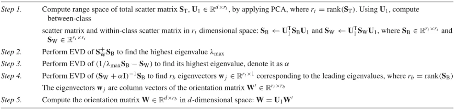
Table 1 Computation of the orientation matrix W using improved RLDA technique

Step 1. Compute range space of total scatter matrix ST, U1∈Rd×rt, by applying PCA, where rt=rank(ST). Using U1, compute between-class

scatter matrix and within-class scatter matrix in rtdimensional space: SB←U1TSBU1and SW←UT1SWU1, where SB∈Rrt×rt and SW∈Rrt×rt

Step 2. Perform EVD of S+_WSBto find the highest eigenvalueλmax

Step 3. Perform EVD of(1/λmaxSB−SW)to find its highest eigenvalue, denote it asα Step 4. Perform EVD of(S_W+αI)−1_S

Bto find rbeigenvectors wj∈Rrt×1corresponding to the leading eigenvalues, where rb=rank(SB) The eigenvectors wjare column vectors of the orientation matrix W∈Rrt×rb

Step 5. Compute the orientation matrix W∈Rd×rb_{in d-dimensional space: W}=_U

1W

where

λ

=

0 is the Lagrange’s multiplier. Equation

3

is

the Lagrange’s function where we are interested in finding

the parameters (w

, λ)

that maximizes function f under the

constrained curve g. Substituting f

=

w

T

S

B

w and g

=

w

T

(

S

W

+

α

I

)

w

−

c in Eq.

3

, we get

2S

B

w

=

λ(

2S

W

w

+

2

α

w

),

or

1

λ

S

B

−

S

W

w

=

α

w

.

(4)

The value of

α

w can be substituted in the constraint function

g, this will give us,

w

T

S

B

w

=

λ

c

.

(5)

Also from the constraint function w

T

(

S

W

+

α

I

)

w

−

c

=

0,

we get w

T

S

ˆ

W

w

=

c. Dividing this term in Eq.

5

, we get

λ

=

w

T

S

B

w

w

T

_S

ˆ

W

w

.

(6)

We can observe the following things from Eq.

6

: 1) the

left-hand term is the Lagrange’s multiplier (in Eq.

4

), and 2)

the right-hand side is same as the Fisher’s modified criterion

defined in Eq.

2

. In order to obtain the value of

λ

in Eq.

6

,

we need to estimate

S

ˆ

W

. If the matrix is not regularize (i.e.,

α

=

0

)

then

S

ˆ

W

=

S

W

. By this substitution, we can obtain

approximate value of

λ

by maximizing w

T

S

B

w

/

w

T

S

W

w.

Now to find the maximum value ow

T

S

B

w

/

w

T

S

W

wf, we

must have eigenvector w corresponding to the leading

eigen-value of S

−_W1

S

B

. However, since S

W

is singular and

non-invertible, S

+_W

can be used in place of S

−_W1

, where S

+_W

is the

pseudoinverse of S

W

. From the EVD of S

+W

S

B

, we can find

λmax

which is the largest eigenvalue of S

+_W

S

B

. The value of

λmax

can be substituted in Eq.

4

(where

λ

=

λmax)

, this will

enable us to find the value of

α

by doing EVD of

(

1_λ

S

B

−

S

W)

.

If r

b

=

rank

(

S

B)

then EVD of

(

1_λ

S

B

−

S

W)

will give r

b

finite

eigenvalues. Since the leading eigenvalue will correspond to

the most discriminant eigenvector [

11

,

32

],

α

is taken to be

the leading eigenvalue. Once the value of

α

is determined,

the orientation vector w can be solved from

(

S

W

+

α

I

)

−1

S

B

w

=

γ

w

.

(7)

It can be shown from Lemma

1

that for improved RLDA

technique, its maximum eigenvalue is approximately equal

to the highest (finite) eigenvalue of Fisher’s criterion.

Lemma 1 The highest eigenvalue of improved RLDA is

approximately equivalent to the highest (finite) eigenvalue

of Fisher’s criterion.

Proof 1 From Eq.

7

,

S

B

w

j

=

γ

j

(

S

W

+

α

I

)

w

j

,

(8)

where

α

is the maximum eigenvalue of

(

1

/λmax

S

B

−

S

W)

(from Eq.

4

);

λmax

≥

0 is approximately the highest

eigen-value of Fisher’s criterion w

T

S

B

w

/

w

T

S

W

w (since

λmax

is

the largest eigenvalue of S

+_W

S

B)

[

22

]; j

=

1

. . .

r

b

and

r

b

=

rank

(

S

B)

. Substituting

α

w

=

(

1

/λmax

S

B

−

S

W)

w

(from Eq.

4

, where

λ

=

λmax)

into Eq.

8

, we get,

S

B

w

m

=

γ

m

S

W

w

m

+

γ

m

(

1

/λmax

S

B

−

S

W)

w

m

,

or

(λmax

−

γ

m

)

S

B

w

m

=

0

where

γ

m

=

max

(γ

j

)

and w

m

is the corresponding

eigen-vector. Since S

B

w

m

=

0 (from Eq.

5

),

γ

m

=

λmax

and

γ

j

< λmax

, where j

=

m. This concludes the proof.

Corollary 1 The value of regularization parameter is

non-negative; i.e.,

α

≥

0 for r

_w

≤

r

t

, where r

t

=

rank

(

S

T)

and

r

_w

=

rank

(

S

W)

.

Proof Please see Appendix C.

Computing Eq.

7

for all the values of

γ

will give the

ori-entation matrix W

∈

R

rt×rb

,

_{having w as its column vectors.}

The orientation matrix W is in r

t

-dimensional space,

how-ever, it can be transformed to d-dimensional space by W

←

U

1

W. Therefore, we get W

∈

R

d×rb

. Let a column vector

w

∈

W be used to transform d-dimensional space to

one-dimensional space and x

∈

X be any feature vector, we have

y

=

w

T

x

,

or y

=

d

i₌1

w

i

x

i

,

(9)

Table 2 The classification accuracy of various feature selection

methods using four distinct classifiers on the SRBCT dataset J4.8 (%) Naïve Bayes (%) kNN (%) SVM pairwise (%) Baseline accuracy 37 37 37 37 Information gain 68 68 90 90 Twoing rule 64 73 86 82 Sum minority 68 68 90 86 Max minority 46 78 90 90 Gini index 64 78 90 90 Sum of variances 54 64 90 86 t-statistic 54 64 90 86 One-dimensional SVM 54 64 90 86 Lasso 90 70 80 75 Filter MRMR 65 35 55 85 Improved RLDA 75 90 95 100

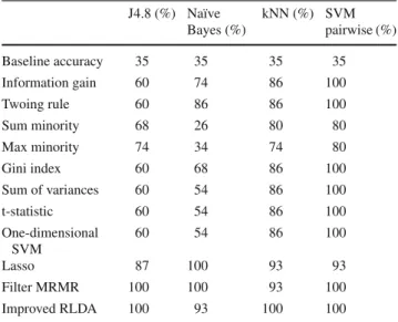
Table 3 The classification accuracy of various feature selection

methods using four distinct classifiers on the MLL dataset J4.8 (%) Naïve Bayes (%) kNN (%) SVM pairwise (%) Baseline accuracy 35 35 35 35 Information gain 60 74 86 100 Twoing rule 60 86 86 100 Sum minority 68 26 80 80 Max minority 74 34 74 80 Gini index 60 68 86 100 Sum of variances 60 54 86 100 t-statistic 60 54 86 100 One-dimensional SVM 60 54 86 100 Lasso 87 100 93 93 Filter MRMR 100 100 93 100 Improved RLDA 100 93 100 100

where

w

i

and x

i

are the elements of w and x, respectively. It

can be envisaged that if

|w

i

x

i

| ≈

0 (where

| · |

is the absolute

value), then the i th element is not contributing for the value

of y in Eq.

9

; i.e., it can be discarded without sacrificing much

information. This concept can be extended for the orientation

matrix W and dataset X as

z

i

=

rb

k=1 n

j=1

|w

i k

x

i j

|

(10)

where i

=

1

,

2

, . . . ,

d. If z

i

≈

0, then i th feature can be

discarded. Equation

10

can be applied recursively to discard

unimportant features as follows:

Table 4 The classification accuracy of various feature selection

methods using four distinct classifiers on the Acute Leukemia dataset J4.8 (%) Naïve Bayes (%) kNN (%) SVM pairwise (%) Baseline accuracy 71 71 71 71 Information gain 91 100 97 97 Twoing rule 91 97 97 97 Sum minority 91 97 97 97 Max minority 91 97 97 97 Gini index 91 97 97 97 Sum of variances 91 97 97 97 t-statistic 91 100 97 97 One-dimensional SVM 91 85 88 97 Lasso 91 94 85 91 Filter MRMR 65 71 74 86 Improved RLDA 94 94 85 100

Step 0. Define q

∈

(

n

,

d

)

2

and set l

=

d.

Step 1. Compute W

∈

R

l×rb

_{(see Table}

₁

_).

Step 2. Compute z

i

using Eq.

10

for i

=

1

,

2

, . . . ,

l.

Step 3. Sort z

i

in descending order; i.e., if s

=

sort

(

z

i

)

then

s

1

>

s

2

>

· · ·

>

s

l

.

Step 4. Discard least important feature corresponding to s

l

.

Let the cardinality of the remaining feature set be

l

−

1 and data subset be X

l−1

∈

R

l×n

.

Step 5. Conduct X

←

X

l−1

and l

←

l

−

1.

Step 6. Continue Steps 1-5 until l

=

q.

The above process will give q-features with the data subset

X

q

∈

R

q×n

, which can be used by a classifier to obtain

classification performance.

The computational requirement for Step 1 of the technique

(Table

1

) would be O

(

dn

2

)

; for Step 2 would be O

(

n

3

)

; for

Step 3 would be O

(

n

3

)

; for Step 4 would be O

(

n

3

)

; and, for

Step 5 would be O

(

dn

2

)

. Therefore, the total estimated for

SSS case (d

n

)

would be O

(

dn

2

)

. If the q features are

to be selected from the total d features then total estimated

computational complexity would be O

(

dn

2

(

d

−

l

))

.

4 Experimentation

In this experiment, we have utilized three DNA microarray

gene expression datasets.

3

The description of these datasets

is given as follows.

2 _{Since RLDA or Improved RLDA is a method for solving small sample} size (SSS) problem, the value of q has to be in (n,d).

3 _{Most of the datasets are downloaded from the Kent Ridge} Bio-medical Dataset (KRBD) (http://datam.i2r.a-star.edu.sg/datasets/ krbd/). The datasets are transformed or reformatted and made available

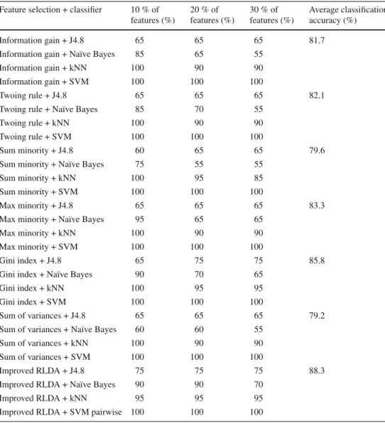
Table 5 The classification

accuracy as a function of the number of selected features of Improved RLDA and several feature selection methods using four distinct classifiers on the SRBCT dataset

Feature selection + classifier 10 % of features (%) 20 % of features (%) 30 % of features (%) Average classification accuracy (%) Information gain + J4.8 65 65 65 81.7

Information gain + Naïve Bayes 85 65 55

Information gain + kNN 100 90 90

Information gain + SVM 100 100 100

Twoing rule + J4.8 65 65 65 82.1

Twoing rule + Naïve Bayes 85 70 55

Twoing rule + kNN 100 90 90

Twoing rule + SVM 100 100 100

Sum minority + J4.8 60 65 65 79.6

Sum minority + Naïve Bayes 75 55 55

Sum minority + kNN 100 95 85

Sum minority + SVM 100 100 100

Max minority + J4.8 65 65 65 83.3

Max minority + Naïve Bayes 95 65 65

Max minority + kNN 100 90 90

Max minority + SVM 100 100 100

Gini index + J4.8 65 75 75 85.8

Gini index + Naïve Bayes 90 70 65

Gini index + kNN 100 95 95

Gini index + SVM 100 100 100

Sum of variances + J4.8 65 65 65 79.2

Sum of variances + Naïve Bayes 60 60 55

Sum of variances + kNN 100 90 90

Sum of variances + SVM 100 100 100

Improved RLDA + J4.8 75 75 75 88.3

Improved RLDA + Naïve Bayes 90 90 70

Improved RLDA + kNN 95 95 95

Improved RLDA + SVM pairwise 100 100 100

SRBCT dataset [

20

] The small round blue-cell tumor

dataset consists of 83 samples with each having 2308 genes.

This is a four class classification problem. The tumors are

Burkitt lymphoma (BL), the Ewing family of tumors (EWS),

neuroblastoma (NB) and rhabdomyosarcoma (RMS). There

are 63 samples for training and 20 samples for testing. The

training set consists of 8, 23, 12 and 20 samples of BL, EWS,

NB and RMS, respectively. The test set consists of 3, 6, 6 and

5 samples of BL, EWS, NB and RMS, respectively.

MLL Leukemia dataset [

2

] This dataset has three classes

namely ALL, MLL and AML. The training set contains 57

leukemia samples (20 ALL, 17 MLL and 20 AML) whereas

Footnote 3 continued

by KRBD repository and we have used them without any further pre-processing. Some datasets which are not available on KRBD repository are downloaded and directly used from respective authors’ supplement link. The URL addresses for all the datasets are given in the Reference Section.

the test set contains 15 samples (4 ALL, 3 MLL and 8 AML).

The dimension of the MLL dataset is 12582.

Acute Leukemia dataset [

13

] This dataset consists of DNA

microarray gene expression data of human acute leukemia

for cancer classification. Two types of acute leukemia data

are provided for classification namely acute lymphoblastic

leukemia (ALL) and acute myeloid leukemia (AML). The

dataset is subdivided into 38 training samples and 34 test

samples. The training set consists of 38 bone marrow samples

(27 ALL and 11 AML) over 7129 probes. The test set consists

of 34 samples with 20 ALL and 14 AML, prepared under

different experimental conditions. All the samples have 7129

dimensions and all are numeric.

The classification performance of the proposed feature

selection method has been gauged by using the above

three datasets. Tables

2

,

3

and

4

show classification

accu-racy of the proposed method compared with several other

existing feature selection methods on the SRBCT, MLL

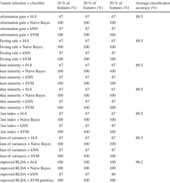
Table 6 The classification

accuracy as a function of the number of selected features of Improved RLDA and several feature selection methods using four distinct classifiers on the MLL dataset

Feature selection + classifier 10 % of features (%) 20 % of features (%) 30 % of features (%) Average classification accuracy (%) Information gain + J4.8 67 67 67 88.5

Information gain + Naïve Bayes 100 100 100

Information gain + kNN 87 87 87

Information gain + SVM 100 100 100

Twoing rule + J4.8 67 67 67 88.5

Twoing rule + Naïve Bayes 100 100 100

Twoing rule + kNN 87 87 87

Twoing rule + SVM 100 100 100

Sum minority + J4.8 67 67 67 88.5

Sum minority + Naïve Bayes 100 100 100

Sum minority + kNN 87 87 87

Sum minority + SVM 100 100 100

Max minority + J4.8 67 67 67 88.5

Max minority + Naïve Bayes 100 100 100

Max minority + kNN 87 87 87

Max minority + SVM 100 100 100

Gini index + J4.8 67 67 67 88.5

Gini index + Naïve Bayes 100 100 100

Gini index + kNN 87 87 87

Gini index + SVM 100 100 100

Sum of variances + J4.8 67 67 67 88.5

Sum of variances + Naïve Bayes 100 100 100

Sum of variances + kNN 87 87 87

Sum of variances + SVM 100 100 100

Improved RLDA + J4.8 100 100 100 96.2

Improved RLDA + Naïve Bayes 100 100 100

Improved RLDA + kNN 87 87 80

Improved RLDA + SVM pairwise 100 100 100

and Acute Leukemia datasets, respectively.

4

Four

classi-fiers from WEKA (

http://www.cs.waikato.ac.nz/ml/weka/

)

used are J4.8, Naïve Bayes, kNN (where k

=

1) and SVM

pairwise. The classification accuracy for the SRBCT and

MLL datasets is obtained from [

40

]. For all the datasets,

the features are ranked by Rankgene program [

38

]. The

Rankgene program computes the features for the following

feature selection methods: Information gain, Twoing rule,

Sum minority, Max minority, Gini index, Sum of variances,

t-statistic and one-dimensional SVM [

38

]. For all the datasets

150 genes are selected as selected by [

40

]. In addition, Lasso

[

42

] and filter MRMR [

26

] are used for feature selection. The

Lasso method deflates the collinearity effect on the features.

It produces sparse parameters that can be used to identify

4_{The cross-validation-based results are shown in Appendix A. The} comparison of improved RLDA with different values of regularization parameter has been shown in Appendix B.

important genes. The number of features selected by Lasso

on SRBCT, MLL and Acute Leukamia is 38, 39 and 16,

5

respectively. The filter MRMR method select features based

on maximal statistical dependency criterion based on mutual

information. It can be observed from Table

2

that the

pro-posed method achieves 75 % classification accuracy using

the J4.8 classifier; 90 % classification accuracy using the

Naïve Bayes classifier; 95 % classification accuracy using

the kNN classifier and 100 % classification accuracy by the

SVM pairwise classifier. In the three out of four cases, the

classification accuracy obtained by improved RLDA is the

highest. Similarly, the classification accuracy on the MLL

dataset (Table

3

) is the highest for improved RLDA in three

5 _{Note that for all the feature selection methods except Lasso method} the number of selected features is 150 (in Tables2,3and4). The Lasso method itself obtains the optimal number of selected features and there-fore cannot be adjusted for a predefined number of selected features.

Table 7 The classification

accuracy as a function of the number of selected features of Improved RLDA and several feature selection methods using four distinct classifiers on the Acute Leukemia dataset

Feature selection + classifier 10 % of features (%) 20 % of features (%) 30 % of features (%) Average classification accuracy (%) Information gain + J4.8 91 91 91 90.6

Information gain + Naïve Bayes 97 100 100

Information gain + kNN 77 79 79

Information gain + SVM 97 94 91

Twoing rule + J4.8 91 91 91 89.1

Twoing rule + Naïve Bayes 94 97 97

Twoing rule + kNN 77 76 79

Twoing rule + SVM 97 91 88

Sum minority + J4.8 91 91 91 88.3

Sum minority + Naïve Bayes 94 97 97

Sum minority + kNN 77 73 73

Sum minority + SVM 97 91 88

Max minority + J4.8 91 91 91 89.2

Max minority + Naïve Bayes 94 97 97

Max minority + kNN 77 77 79

Max minority + SVM 97 91 88

Gini index + J4.8 91 91 91 88.0

Gini index + Naïve Bayes 94 97 97

Gini index + kNN 79 70 70

Gini index + SVM 97 91 88

Sum of variances + J4.8 91 91 91 89.2

Sum of variances + Naïve Bayes 94 97 97

Sum of variances + kNN 77 77 79

Sum of variances + SVM 97 91 88

Improved RLDA + J4.8 91 91 91 92.5

Improved RLDA + Naïve Bayes 97 100 100

Improved RLDA + kNN 88 79 82

Improved RLDA + SVM pairwise 97 97 97

out of four cases method when compared with several other

feature selection methods using four distinct classifiers. On

the Acute Leukemia dataset (Table

4

), the classification

accu-racy of improved RLDA is the highest for the J4.8 classifier

(94 %) and the SVM pairwise classifier (100 %). In total

of 12 cases (Tables

2

–

4

), improved RLDA is giving highest

results in eight cases. It can, therefore, be concluded that the

proposed method is exhibiting promising results.

Next, we considered different number of selected features

by Improved RLDA and several feature selection method,

and shown the evolution of the performance of the classifiers

with respect to the number of selected features. The results

are shown in Tables

5

,

6

and

7

. It can be observed from the

Tables

5

–

7

that in most of the cases the average

classifica-tion accuracy for Improved RLDA is consistently higher than

other feature selection methods.

Furthermore, we conducted experiments to see the

bio-logical significance of the selected features by the proposed

method. We use SRBCT data as a prototype to show the

biological significance using Ingenuity Pathway Analysis.

6

The selected 150 features from the proposed algorithm are

6 _{Ingenuity Pathway Analysis (IPA) (http://www.ingenuity.com) is a} software that helps researchers to model, analyze, and understand the complex biological and chemical systems at the core of life science research. IPA has been broadly adopted by the life science research community. IPA helps to understand complex ’omics data at multi-ple levels by integrating data from a variety of experimental platforms and providing insight into the molecular and chemical interactions, cel-lular phenotypes, and disease processes of the system. IPA provides insight into the causes of observed gene expression changes and into the predicted downstream biological effects of those changes. Even if the experimental data is not available, IPA can be used to intelligently search the Ingenuity Knowledge Base for information on genes, pro-teins, chemicals, drugs, and molecular relationships to build biologi-cal models or to get up to speed in a relevant area of research. IPA provides the right biological context to facilitate informed decision-making, advance research project design, and generate new testable hypotheses.

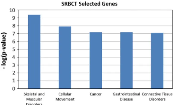
Fig. 1 Top five high-level biological function on selected 150 genes

of SRBCT by improved RLDA-based feature selection method

used for this purpose. Out of 150 genes, 10 genes were

found unmapped in IPA. The top five high-level biological

functions obtained are shown in Fig.

1

. In the figure, the

y axis denotes the negative of logarithm of p-values and

x axis denotes the high level functions. Since the cancer

function is of paramount interest, we investigated them

fur-ther. There are 61 cancer sub-functions obtained from the

experiment. Top 25 cancer sub-functions with significant

p-values are shown in Table

8

. In IPA, the p-value reflects the

enrichment of a given function to a set of focused genes.

The smaller the p-value is, the less likely that the

associ-ation is random, and the more significant the associassoci-ation.

In general p-values less than 0.05 indicate a statistically

significant, non-random association. The p-value is

calcu-lated using the right-tailed Fisher exact test (IPA, Available

at:

http://www.ingenuity.com

) [

28

,

29

]. In the table, the

p-values and the number of selected genes are depicted

cor-responding to the selected functions. The selected genes

by the proposed method provide significant p-values above

the threshold (as specified in IPA). This shows that the

features selected by the proposed method contain useful

information for discriminatory purpose and have biological

significance.

We have also carried out sensitivity analysis to check the

robustness of the proposed method. For this purpose, we use

the SRBCT dataset as a prototype and select top 100 genes.

After this selection, we contaminate the dataset by adding

Gaussian noise, then applied the method again to find the top

100 genes. The generated noise levels are 1, 2 and 5 % of the

standard deviation of the original gene expression values. The

number of genes which are common after contamination and

before contamination is noted. This contamination of data

and selection of genes are repeated 20 times. The average

number of genes over 20 iterations is depicted in Fig.

2

. It

can be observed from the figure that the proposed method is

able to capture the majority of the original genes in the noisy

environmental condition.

Table 8 Cancer sub-functions

Functions p value # Selected

genes Metastatic colorectal cancer 6.99E−08 12

Tumorigenesis 1.01E−07 62

Neoplasia 5.05E−07 59

Cancer 6.97E−07 58

Uterine cancer 2.87E−06 19

Benign tumor 3.75E−06 17

Leiomyomatosis 1.06E−05 12

Carcinoma 1.11E−05 47

Adenocarcinoma 1.81E−05 17

Gastrointestinal tract cancer 2.60E−05 24

Colorectal cancer 3.46E−05 22

Uterine leiomyoma 5.62E−05 10

Metastasis 6.11E−05 13

Genital tumor 6.69E−05 22

Prostate cancer 1.42E−04 16

Trisomy 8 myelodysplastic syndrome 2.25E−04 2 Central nervous system tumor 2.87E−04 10

Digestive organ tumor 3.21E−04 27

Breast cancer 3.41E−04 20

Brain cancer 4.28E−04 9

Leukemia 6.88E−04 11

Hematologic cancer 7.14E−04 14

Endometrial carcinoma 8.86E−04 8

Neuroblastoma 1.25E−03 5

Hematological neoplasia 1.38E−03 15

Endocrine gland tumor 1.42E−03 11

Tumorigenesis of carcinoma 1.54E−03 2

B-cell leukemia 1.68E−03 6

Entrance of tumor cell lines 2.04E−03 2

Endometrial cancer 2.12E−03 7

In order to check the sensitivity analysis with respect

to the classification accuracy, we contaminated the dataset

by adding Gaussian noise (as above) and selected 150

fea-tures using the improved RLDA technique. The

classifica-tion accuracy is obtained by using the SVM-pairwise

classi-fier. The results are shown in Table

9

. It can observed from

Table

9

that for low level noise the degradation in

classifi-cation performance is not enough. But when the noise level

increases the classification accuracy deteriorates (especially

on the MLL dataset and the Acute Leukemia dataset).

Next, we carried out experimentation to obtain ROC curve

and AUC analysis. For the ROC curve, we use

sensitiv-ity and specificsensitiv-ity as the two measures. The sensitivsensitiv-ity is

given as True Positive

/(

True Positive

+

False Negative

)

and

the specificity is given as True negative

/(

True Negative

+

False Positive

)

. We varied the noise level and select 150

84 86 88 90 92 94 96 98 100 1 2 3 4 5

Average number of common genes

Added noise in percentage

Fig. 2 Sensitivity analysis for the proposed feature selection method

on the SRBCT dataset at different noise levels. The y axis depicts the average number of common genes over 20 iterations and x axis depicts the added noise in percentage

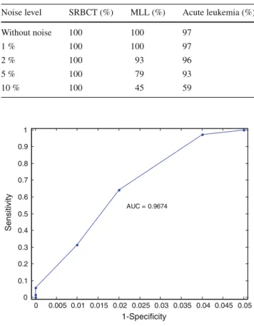
Table 9 Sensitivity analysis with respect to classification accuracy on

the SRBCT, MLL and Acute Leukemia dataset

Noise level SRBCT (%) MLL (%) Acute leukemia (%)

Without noise 100 100 97 1 % 100 100 97 2 % 100 93 96 5 % 100 79 93 10 % 100 45 59 0 0.005 0.01 0.015 0.02 0.025 0.03 0.035 0.04 0.045 0.05 0 0.1 0.2 0.3 0.4 0.5 0.6 0.7 0.8 0.9 1 1-Specificity Sensitivity AUC = 0.9674

Fig. 3 The ROC curve

genes using improved RLDA and then use SVM-pairwise to

compute sensitivity and specificity. The ROC curve is shown

in Fig.

3

. This curve shows the trade-off between

sensitiv-ity and specificsensitiv-ity. The AUC provides the overall accuracy

and is a useful parameter for comparing the performance.

The high value of AUC parameter indicates high

accu-racy. The value of AUC is computed to be 0

.

9674 which is

promising.

5 Conclusion

In this paper, we presented a feature selection method using

improved regularized linear discriminant analysis technique.

Three DNA microarray gene expression datasets have been

utilized to see the performance of the proposed method. It

was observed that the method is achieving encouraging

clas-sification accuracy using small number of selected gene.

The biological significance has also been demonstrated by

performing functional analysis. Moreover, robustness of the

method was exhibited by conducting sensitivity analysis and

encouraging results are obtained. The sensitivity analysis

with respect to classification accuracy and ROC curve have

also been discussed.

Appendix A

In this section, we use cross-validation procedure to compute

average classification accuracy using four distinct classifiers

and the proposed feature selection method. Three datasets

have been used for this purpose are SRBCT, MLL and Acute

Leukemia. The classification accuracy using fold k

=

5 and

fold k

=

10 are given in Tables

10

,

11

and

12

. It can be

observed that the classification accuracy obtained by k-fold

cross-validation procedure is comparably similar to the

clas-sification accuracy obtained in Tables

2

-

4

.

Table 10 k-fold cross-validation using improved RLDA and four

dis-tinct classifiers on the SRBCT dataset

Fold J4.8 Naïve bayes kNN SVM pairwise

k=5 80 % 89 % 92 % 100 %

k=10 88 % 92 % 95 % 100 %

Table 11 k-fold cross-validation using improved RLDA and four

dis-tinct classifiers on the MLL dataset

Fold J4.8 Naïve bayes kNN SVM pairwise

k=5 91 % 94 % 94 % 95 %

k=10 87 % 93 % 95 % 97 %

Table 12 k-fold cross-validation using improved RLDA and four

dis-tinct classifiers on the Acute Leukemia dataset

Fold J4.8 Naïve bayes kNN SVM pairwise

k=5 91 % 97 % 87 % 94 %

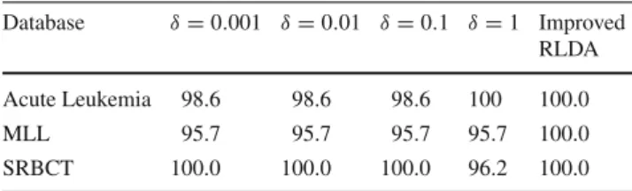
Table 13 Classification accuracy (in percentage) of RLDA and improved RLDA Database δ=0.001 δ=0.01 δ=0.1 δ=1 Improved RLDA Acute Leukemia 98.6 98.6 98.6 100 100.0 MLL 95.7 95.7 95.7 95.7 100.0 SRBCT 100.0 100.0 100.0 96.2 100.0

The highest classification accuracies obtained are depicted in bold fonts

Appendix B

In this appendix, we compare different values of

regulariza-tion parameter with the proposed improved RLDA technique.

In order to show this, we computed classification accuracy

on four different values of

α

for RLDA technique. These

are

δ

= [

0

.

001

,

0

.

01

,

0

.

1

,

1

]

, where

α

=

δ

∗

λW

and

λW

is

the maximum eigenvalue of within-class scatter matrix. We

applied threefold cross-validation procedure on a number of

datasets and shown the results in columns 2–5 of Table

11

.

The last column of the table denotes the classification

accu-racy using improved RLDA technique (Table

13

).

It can be observed from the table that the different

val-ues of the regularization parameter give different

classifica-tion accuracies and therefore, the choice of the regularizaclassifica-tion

parameter affects the classification performance. Thus, it is

important to select the regularization parameter correctly to

get the good classification performance. It can be observed

that for all the datasets, the proposed technique is exhibiting

promising results.

Appendix C

Corollary 1 The value of regularization parameter is

non-negative; i.e.,

α

≥

0 for r

_w

≤

r

t

, where r

t

=

rank

(

S

T)

and

r

_w

=

rank

(

S

W)

.

Proof From Eq.

2

, we can write

J

=

w

T

_S

B

w

w

T

₍

_S

W

+

α

I

)

w

,

(11)

where S

B

∈

R

rt×rt

and S

W

∈

R

rt×rt

. We can rearrange the

above expression as

w

T

S

B

w

=

J w

T

(

S

W

+

α

I

)

w

(12)

The eigenvalue decomposition (EVD) of S

W

matrix

(assuming r

_w

<

r

t

)

can be given as S

W

=

U

2

U

T

,

where

U

∈

R

rt×rt

_{is an orthogonal matrix,}

2

=

2 w 0 0 0

∈

R

rt×rt

and

_w

=

diag

(

q

₁2

,

q

₂2

, . . . ,

q

_r2_w

)

∈

R

rw×r_w

_are

diago-nal matrices (as r

_w

<

r

t

)

. The eigenvalues q

_k2

>

0 for

k

=

1

,

2

, . . . ,

r

_w

. Therefore,

S

W

=

(

S

W

+

α

I

)

=

UDU

T

,

where D

=

2

+

α

I

or D

−1/2

U

T

S

W

UD

−1/2

=

I

(13)

The between class scatter matrix S

B

can be transformed

by multiplying UD

−1/2

on the right side and D

−1/2

U

T

on

the left side of S

B

as D

−1/2

U

T

S

B

UD

−1/2

. The EVD of this

matrix will give

D

−1/2

U

T

S

B

UD

−1/2

=

ED

B

E

T

,

(14)

where E

∈

R

rt×rt

_{is an orthogonal matrix and D}

B

∈

R

rt×rt

is a diagonal matrix. Equation

14

can be rearranged as

E

T

D

−1/2

U

T

S

B

UD

−1/2

E

=

D

B,

(15)

Let the leading eigenvalue of D

B

is

γ

and its corresponding

eigenvector is e

∈

E. Then Eq.

15

can be rewritten as

e

T

D

−1/2

U

T

S

B

UD

−1/2

e

=

γ,

(16)

The eigenvector e can be multiplied right side and e

T

on left

side of Eq.

13

, we get

e

T

D

−1/2

U

T

S

_W

UD

−1/2

e

=

1

(17)

It can be seen from Eqs.

13

and

15

that matrix W

=

UD

−1/2

E diagonalizes both S

B

and S

W

, simultaneously.

Also vector w

=

UD

−1/2

e simultaneously gives

γ

and unity

eigenvalue in Eqs.

16

and

17

. Therefore, w is a solution of

Eq.

12

. Substituting w

=

UD

−1/2

e in Eq.

12

, we get J

=

γ

;

i.e., w is a solution of Eq.

12

.

From Lemma

1

, the maximum eigenvalue of expression

(

S

W

+

α

I

)

−1

S

B

w

=

γ

w is

γ

m

=

λmax

>

0 (i.e., real,

pos-itive and finite). Therefore, the eigenvectors corresponding

to this positive

γ

m

should also be in real hyperplane (i.e., the

components of the vector w have to have real values). Since

w

=

UD

−1/2

e with w to be in real hyperplane, we must have

D

−1/2

to be real.

Since D

=

2

+

α

I

=

diag

(

q

₁2

+

α,

q

₂2

+

α, . . . ,

q

_r2_w

+

α, α, . . . , α)

, we have

D

−1/2

=

diag

(

1

/

q

₁2

+

α,

1

/

q

₂2

+

α, . . . ,

1

/

q

2 r_w

+

α,

1

/

√

α, . . . ,

1

/

√

α).

Therefore, the elements of D

−1/2

, must satisfy 1

/

q

_k2

+

α >

0 and 1

/

√

α >

0 for k

=

1

,

2

, . . . ,

r

_w

(note r

_w

<

r

t

)

; i.e.,

α

cannot be negative or

α >

0. Furthermore, if r

_w

=

r

t

then

matrix S

W

will be a non-singular matrix and its inverse will

exist. In this case, regularization is not required and therefore

α

=

0. Thus,

α

≥

0 for r

_w

≤

r

t

. This concludes the proof.

References

1. Anton, H.: Calculus. Wiley, New York (1995)

2. Armstrong, S.A., Staunton, J.E., Silverman, L.B., Pieters, R., den Boer, M.L., Minden, M.D., Sallan, S.E., Lan-der, E.S., Golub, T.R., Korsemeyer, S.J.: MLL translocations

specify a distinct gene expression profile that distinguishes a unique leukemia. Nat. Genet. 30, 41–47 (2002). [Data Source1: http://sdmc.lit.org.sg/GEDatasets/Datasets.html] [Data Source2: http://www.broad.mit.edu/cgi-bin/cancer/publications/ pub_paper.cgi?mode=view&paper_id=63]

3. Banerjee, M., Mitra, S., Banka, H.: Evolutinary-rough feature selection in gene expression data. IEEE Trans. Syst. Man Cybern. Part C Appl. Rev. 37, 622–632 (2007)

4. Cong G., Tan K.-L., Tung A.K.H., Xu X.: Mining top-k cover-ing rule groups for gene expression data. In: The ACM SIGMOD International Conference on Management of Data, pp. 670–681 (2005)

5. Dai, D.Q., Yuen, P.C.: Regularized discriminant analysis and its application to face recognition. Pattern Recognit. 36(3), 845–847 (2003)

6. Dai, D.Q., Yuen, P.C.: Face recognition by regularized discriminant analysis. IEEE Trans. SMC 37(4), 1080–1085 (2007)

7. Ding, C., Peng, H.: Minimum redundancy feature selection from microarray gene expression data. J. Bioinf. Comput. Biol. 523–529 (2003)

8. Duda, R.O., Hart, P.E.: Pattern Classification and Scene Analysis. Wiley, New York (1973)

9. Dudoit, S., Fridlyand, J., Speed, T.P.: Comparison of discriminant methods for the classification of tumors using gene expression data. J. Am. Stat. Assoc. 97, 77–87 (2002)

10. Friedman, J.H.: Regularized discriminant analysis. J. Am. Stat. Assoc. 84(405), 165–175 (1989)

11. Fukunaga, K.: Introduction to Statistical Pattern Recognition. Aca-demic Press, London (1990)

12. Furey, T.S., Cristianini, N., Duffy, N., Bednarski, D.W., Schum-mer, M., Haussler, D.: Support vector machine classification and validation of cancer tissue samples using microarray expression data. Bioinformatics 16(10), 906–914 (2000)

13. Golub, T.R., Slonim, D.K., Tamayo, P., Huard, C., Gaasenbeek, M., Mesirov, J.P., Coller, H., Loh, M.L., Downing, J.R., Caligiuri, M.A., Bloomfield, C.D., Lander E.S.: Molecular classification of cancer: class discovery and class prediction by gene expression monitoring. Science 286, 531–537 (1999). [Data Source:http:// datam.i2r.a-star.edu.sg/datasets/krbd/]

14. Guo, Y., Hastie, T., Tibshirani, R.: Regularized discriminant analy-sis and its application in microarrays. Biostatistics 8(1), 86–100 (2007)

15. Guyon, I., Weston, J., Barnhill, S., Vapnik, V.: Gene selection for cancer classification using support vector machines. Mach. Learn.

46, 389–422 (2002)

16. Hastie, T., Tibshirani, R., Friedman, J.: The elements of statistical learning. Springer, NY (2001)

17. Huang, R., Liu, Q., Lu, H., Ma, S.: Solving the small sample size problem of LDA. Proc. ICPR 3, 29–32 (2002)

18. Huang, Y., Xu, D., Nie, F.: Semi-supervised dimension reduction using trace ratio criterion. IEEE Trans. Neural Netw. Learn. Syst.

23(3), 519–526 (2012)

19. Huang, Y., Xu, D., Nie, F.: Patch distribution compatible semi-supervised dimension reduction for face and human gait recogni-tion. IEEE Trans. Circuits Syst. Video Technol. 22(3), 479–488 (2012)

20. Khan, J., Wei, J.S., Ringner, M., Saal, L.H., Ladanyi, M., Wester-mann, F., Berthold, F., Schwab, M., Antonescu, C.R., Peterson, C., Meltzer, P.S.: Classification and diagnostic prediction of cancers using gene expression profiling and artificial neural network. Nat. Med. 7, 673–679 (2001). [Data Source:http://research.nhgri.nih. gov/microarray/Supplement/]

21. Li, J., Wong, L.: Using rules to analyse bio-medical data: a comparison between C4.5 and PCL. In: Advances in Web-Age Information Management, pp. 254–265. Springer, Berlin (2003)

22. Liu, J., Chen, S.C., Tan, X.Y.: Efficient pseudo-inverse linear dis-criminant analysis and its nonlinear form for face recognition. Int. J. Patt. Recogn. Artif. Intell. 21(8), 1265–1278 (2007)

23. Nie, F., Huang, H., Cai X., Ding, C.: Efficient and robust feature selection via joint l2,1-norms minimization, NIPS (2010) 24. Pan, W.: A comparative review of statistical methods for

discover-ing differentially expressed genes in replicated microarray experi-ments. Bioinformatics 18, 546–554 (2002)

25. Pavlidis, P., Weston, J., Cai, J. and Grundy, W.N.: Gene functional classification from heterogeneous data. In: International Confer-ence on Computational Biology, pp. 249–255 (2001)

26. Peng, H., Long, F., Dong, C.: Feature selection based on mutual information: criteria of max-dependency, max-relevance, and min-redundancy. IEEE Trans. Pattern Anal. Mach. Intell. 27(8), 1226– 1238 (2005)

27. Saeys, Y., Inza, I., Larrañaga, P.: A review of feature selection techniques in bioinformatics. Bioinformatics 23(19), 2507–2517 (2007)

28. Sharma, A., Imoto, S., Miyano, S.: A top-r feature selection algo-rithm for microarray gene expression data. IEEE/ACM Trans. Computat. Biol. Bioinf. 9(3), 754–764 (2012)

29. Sharma, A., Imoto, S., Miyano, S.: A between-class overlapping filter-based method for transcriptome data analysis. J. Bioinf. Com-putat. Biol. 10(5), 1250010-1–1250010-20 (2012)

30. Sharma, A., Imoto, S., Miyano, S., Sharma, V.: Null space based feature selection method for gene expression data. Int. J. Mach. Learn. Cybern. 3(4), 269–276 (2012). doi: 10.1007/s13042-011-0061-9

31. Sharma, A., Koh, C.H., Imoto, S., Miyano, S.: Strategy of finding optimal number of features on gene expression data. IEE. Electron. Lett. 47(8), 480–482 (2011)

32. Sharma, A., Paliwal, K.K.: Fast principal component analysis using fixed-point algorithm. Pattern Recognit. Lett. 28(10), 1151–1155 (2007)

33. Sharma, A., Paliwal, K.K.: Rotational linear discriminant analy-sis for dimensionality reduction. IEEE Trans. Knowl. Data Eng.

20(10), 1336–1347 (2008)

34. Sharma, A., Paliwal, K.K.: A gradient linear discriminant analysis for small sample sized problem. Neural Process. Lett. 27(1), 17–24 (2008)

35. Sharma, A., Paliwal, K.K.: A new perspective to null linear dis-criminant analysis method and its fast implementation using ran-dom matrix multiplication with scatter matrices. Pattern Recognit.

45, 2205–2213 (2012)

36. Sharma, A., Lyons, J., Dehzangi, A., Paliwal, K.K.: A feature extraction technique using bi-gram probabilities of position spe-cific scoring matrix for protein fold recognition. J. Theoret. Biol.

320(7), 41–46 (2013)

37. Sharma, A., Paliwal, K.K., Imoto, S., Miyano, S., Sharma, V., Ananthanarayanan, R.: A feature selection method using fixed-point algorithm for DNA microarray gene expression data. Int. J. Knowl. Based Intell. Eng. Syst. (2013, accepted)

38. Su, Y., Murali, T.M., Pavlovic, V., Kasif, S.: RankGene: identifica-tion of diagnostic genes based on expression data, Bioinformatics, pp. 1578–1579 (2003)

39. Tan, A.C., Gilbert, D.: Ensemble machine learning on gene expres-sion data for cancer classification. Appl. Bioinf. 2(3 Suppl), S75–83 (2003)

40. Tao, L., Zhang, C., Ogihara, M.: A comparative study of feature selection and multiclass classification methods for tissue classifica-tion based on gene expression. Bioinformatics 20(14), 2429–2437 (2004)

41. Thomas, J., Olson, J.M., Tapscott, S.J., Zhao, L.P.: An efficient and robust statistical modeling approach to discover differentially expressed genes using genomic expression profiles. Genome Res.

42. Tibshirani, R.: Regression shrinkage and selection via the lasso. J. R. Stat. Soc. B 58(1), 267–288 (1996)

43. Wang, A., Gehan, E.A.: Gene selection for microarray data analy-sis using principal component analyanaly-sis. Stat. Med. 24, 2069–2087 (2005)

44. Wu, G., Xu, W., Zhang, Y., Wei, Y.: A preconditioned conjugate gradient algorithm fo GeneRank with application to microarray data mining. Data Mining Knowl. Discov. (2011). doi:10.1007/ s10618-011-0245-7

45. Xu, D., Yan, S.: Semi-supervised bilinear subspace learning. IEEE Trans. Image Process. 18(7), 1671–1676 (2009)

46. Zhou, L., Wang, L., Shen, C., Barnes, N.: Hippocampal shape clas-sification using redundancy constrained feature selection. Medical Image Computing and Computer-Assisted Intervention, MICCAI 2010. In: Lecture Notes in Computer Science, vol. 6362, pp. 266– 273. Springer, Berlin (2010)

Author Biographies

Alok Sharma received the

BTech degree from the Univer-sity of the South Pacific (USP), Suva, Fiji, in 2000 and the MEng degree, with an academic excel-lence award, and the PhD degree in the area of pattern recog-nition from Griffith University, Brisbane, Australia, in 2001 and 2006, respectively. He was with the University of Tokyo, Japan (2010–2012) as a research fel-low. He is an Associate Prof. at the USP and an Adjunct Asso-ciate Prof. at the Institute for Inte-grated and Intelligent Systems (IIIS), Griffith University. He partici-pated in various projects carried out in conjunction with Motorola (Syd-ney), Auslog Pty., Ltd. (Brisbane), CRC Micro Technology (Brisbane), the French Embassy (Suva) and JSPS (Japan). His research interests include pattern recognition, computer security, human cancer classi-fication and protein fold and structural class prediction problems. He reviewed several articles and is in the editorial board of several journals.

Kuldip K. Paliwal received the

B.S. degree from Agra Univer-sity, Agra, India, in 1969, the M.S. degree from Aligarh Mus-lim University, Aligarh, India, in 1971 and the Ph.D. degree from Bombay University, Bom-bay, India, in 1978. He has been carrying out research in the area of speech processing since 1972. He has worked at a number of organizations includ-ing Tata Institute of Fundamental Research, Bombay, India, Nor-wegian Institute of Technology, Trondheim, Norway, University of Keele, U.K., AT & T Bell ratories, Murray Hill, New Jersey, U.S.A., AT & T Shannon Labo-ratories, Florham Park, New Jersey, U.S.A., and Advanced Telecom-munication Research Laboratories, Kyoto, Japan. Since July 1993, he has been a professor at Griffith University, Brisbane, Australia, in the School of Microelectronic Engineering. His current research interests include speech recognition, speech coding, speaker recognition, speech enhancement, face recognition, image coding, bioinformatics, protein

fold and structural class prediction problems, pattern recognition and artificial neural networks. He has published more than 300 papers in these research areas. Prof. Paliwal is a Fellow of Acoustical Society of India. He has served the IEEE Signal Processing Society’s Neural Networks Technical Committee as a founding member from 1991 to 1995 and the Speech Processing Technical Committee from 1999 to 2003. He was an Associate Editor of the IEEE Transactions on Speech and Audio Processing during the periods 1994–1997 and 2003–2004. He also served as Associate Editor of the IEEE Signal Processing Let-ters from 1997 to 2000. He was the editor-in-chief of Speech Com-munication Journal from 2005 to 2011. He is in the editorial board of IEEE Signal Processing Magazine. He was the General Co-Chair of the Tenth IEEE Workshop on Neural Networks for Signal Processing (NNSP2000).

Seiya Imoto is currently an Associate Professor of Human Genome Center, Institute of Medical Science, University of Tokyo. He received the B.S., M.S., and Ph.D. degrees in math-ematics from Kyushu University, Japan, in 1996, 1998 and 2001, respectively. His current research interests cover statistical analy-sis of high-dimensional data by Bayesian approach, biomedical information analysis, microar-ray gene expression data analy-sis, gene network estimation and analysis, data assimilation in biological networks and computational drug target discovery.

Satoru Miyano is a

Profes-sor of Human Genome Cen-ter, Institute of Medical Sci-ence, University of Tokyo. He received the B.S., M.S. and Ph.D. degrees all in mathematics from Kyushu University, Japan, in 1977, 1979 and 1984, respec-tively. His research group is developing computational meth-ods for inferring gene networks from microarray gene expression data and other biological data, e.g., protein-protein interactions, promoter sequences. The group also developed a software tool, Cell Illustrator, for modeling and sim-ulation of various biological systems. Currently, his research group is intensively working for developing the molecular network model of lung cancer by time-course gene expression and proteome data. With these technical achievements, his research direction is now heading toward a creation of Systems Pharmacology. He is Associate Editor of PLoS Computational Biology; IEEE/ACM Transactions on Computa-tional Biology and Bioinformatics; and, Health Informatics. He was Associate Editor of Bioinformatics during 2002–2006 and 2007–2009. He is Editor of Journal of Bioinformatics and Computational Biology; Lecture Notes in Bioinformatics; Advances in Bioinformatics; Jour-nal of Biomedicine and Biotechnology; InternatioJour-nal JourJour-nal of Bioin-formatics Research and Applications (IJBRA); Immunome Research; Theoretical Computer Science; Transactions on Petri Nets and Other Models of Concurrency (ToPNoC); and, New Generation Computing. He is Editor-in-Chief of Genome Informatics. He is recipient of IBM Science Award (1994) and Sakai Special Award (1994).