Recommendation algorithms optimization

doc. Ing. Jan Janoušek, Ph.D. Head of Department

prof. Ing. Pavel Tvrdík, CSc. Dean

C

ZECH

T

ECHNICAL

U

NIVERSITY IN 

P

RAGUE

F

ACULTY OF

I

NFORMATION

T

ECHNOLOGY

ASSIGNMENT OF MASTER’S THESIS

Title: Recommendation algorithms optimization

Student: Bc. Jakub Drdák Supervisor: Ing. Pavel Kordík, Ph.D. Study Programme: Informatics

Study Branch: Knowledge Engineering

Department: Department of Theoretical Computer Science Validity: Until the end of winter semester 2018/19

Instructions

Survey modern scalable recommendation algorithms. Benchmark selected algorithms on 2-3 datasets and identify parameters suitable for optimization. Design and implement an optimization procedure capable of fine-tuning these parameters according to given evaluation measures. Show that your algorithm is able to optimize recommendation algorithms for new datasets.

References

Master’s thesis

Recommendation Algorithms Optimization

Bc. Jakub Drd´

ak

Department of Theoretical Computer Science Supervisor: Ing. Pavel Kord´ık Ph.D.

Acknowledgements

I would like to thank company Recombee for borrowing hardware for testing and my supervisor Ing. Pavel Kord´ık, Ph.D. for consultations and help during the whole study.

Declaration

I hereby declare that the presented thesis is my own work and that I have cited all sources of information in accordance with the Guideline for adhering to ethical principles when elaborating an academic final thesis.

I acknowledge that my thesis is subject to the rights and obligations stip-ulated by the Act No. 121/2000 Coll., the Copyright Act, as amended, in particular that the Czech Technical University in Prague has the right to con-clude a license agreement on the utilization of this thesis as school work under the provisions of Article 60(1) of the Act.

c

2018 Jakub Drd´ak. All rights reserved.

This thesis is school work as defined by Copyright Act of the Czech Republic. It has been submitted at Czech Technical University in Prague, Faculty of Information Technology. The thesis is protected by the Copyright Act and its usage without author’s permission is prohibited (with exceptions defined by the Copyright Act).

Citation of this thesis

Drd´ak, Jakub. Recommendation Algorithms Optimization. Master’s thesis. Czech Technical University in Prague, Faculty of Information Technology, 2018.

Abstrakt

V posledn´ıch letech se vyvinulo velk´e mnoˇzstv´ı rozliˇcn´ych doporuˇcovac´ıch al-goritm˚u. Jednu vˇec maj´ı ale vˇsechny spoleˇcnou. Jejich hyper-parametry se mus´ı peˇclivˇe zvolit, aby dosahovaly dobr´ych v´ysledk˚u.

Tato pr´ace se zab´yv´a v´ybˇerem takov´ych algoritm˚u a navrhnut´ım optimal-izaˇcn´ı procedury, kter´a bude schopn´a nal´ezt vhodn´e hyper-parametry tˇechto algoritm˚u. V´ysledky jsou pak ovˇeˇreny na re´aln´ych datasetech.

Kl´ıˇcov´a slova Rekomendaˇcn´ı syst´emy, hlubok´e uˇcen´ı, hyper-parametrick´a

optimalizace

Abstract

Various recommendation algorithms have been proposed in recent years. How-ever, each of them has one thing in common. It is essential to tune their hyper-parameters in order to achieve good results.

This work has focused on selecting modern and scalable algorithms. The aim has been to design and implement an optimization procedure capable of fine-tuning their hyper-parameters and evaluate the results on real-world datasets.

Contents

Introduction 1

Motivation And Objectives . . . 1

Problem Definition . . . 1

Organisation Of The Thesis . . . 2

1 Survey 3 1.1 Recommender Systems Overview . . . 3

1.2 Recommendation Algorithms . . . 5

1.3 Hyper-parameters Optimization Techniques . . . 14

2 Solution Analysis 17 2.1 Algorithms Analysis . . . 17 2.2 Optimization Procedure . . . 21 3 Realization 25 3.1 Programming Language . . . 25 3.2 Library Usage . . . 25 3.3 Implementation . . . 26 4 Experiments 35 4.1 Datasets . . . 35 4.2 Evaluation Scheme . . . 35 4.3 Experimental Settings . . . 36 4.4 Quantitative Comparison . . . 37 Conclusion 45 Bibliography 47 A Appendix 51

B Acronyms 53

List of Figures

1.1 Recommender System Classification . . . 5

3.1 System Overview . . . 27

3.2 Scalability: number of processes . . . 30

3.3 Scalability: size of latent representation . . . 31

3.4 Scalability: original simplified CDL (loosely dashed) and proposed CDL (solid) implemenation . . . 32

4.1 Coverage-Recall curve . . . 37

4.2 Accuracy: comparison between osCDL and nCDL . . . 38

4.3 CiteULike MF convergence: RS vs. GP . . . 39 4.4 Fashion MF convergence: RS vs. GP . . . 39 4.5 News MF convergence: RS vs. GP . . . 40 4.6 CiteULike CDL convergence: RS vs. GP . . . 40 4.7 Fashion CDL convergence: RS vs. GP . . . 41 4.8 Fashion Recall . . . 41 4.9 Fashion Coverage . . . 42 4.10 News Recall . . . 42 4.11 News Coverage . . . 43 4.12 CiteULike Recall . . . 43 4.13 CiteULike Coverage . . . 44

Introduction

Motivation And Objectives

Recommender systems are literally everywhere around us. They recommend to us how to spend free time, which movie to watch, book to read, what to buy, even which job to choose. Recommendation systems are an essential part of many areas. It is a critical tool to promote sales and services for many online websites and mobile applications.

However, not all companies have resources to develop their own recom-mender system. In many cases, it can be a preferable way to use ready-to-use tools. The company Recommbee offers one of these tools. Recombee provides an intuitive RESTful recommendation API, which is used by various interna-tional internet companies for recommendation to their users. This can lead to an interesting problem. Each company has a different business model, collects different data, offers different products and so on. Such data are a content of Recommbee database.

Therefore, the first goal of this thesis is to select modern and scalable recommendation algorithms, which are able to exploit data and offer an accu-rate recommendation. Further, to design an optimization procedure capable of fine-tuning hyper-parameters selected algorithms and validate results on several real-world datasets.

Problem Definition

The goal is to select modern and scalable recommendation algorithms, design fine-tuning procedure capable to tune hyper-parameters of selected algorithms and this procedure validate on several datasets.

Organisation Of The Thesis

The thesis is structured as follows: Chapter 1 presents a recommender sys-tems overview and survey of selected algorithms together with a brief overview of hyper-parameter optimization techniques. Chapter 2 contains an analysis of chosen algorithms and design of fine-tuning procedure. Following Chap-ter 3 describes an algorithms implementation and the last ChapChap-ter 4 covers experiments.

Chapter

1

Survey

In the survey part we will first look at recommender systems, show their brief overview and describe basic types. Then we will focus on a subset of algorithms, which are suitable for this work. Each selected algorithm will be briefly described as discussed.

Next, we will move focus on hyper-parameter optimization, one of the essential parts of machine learning, although it sometimes suffers from a lack of care. This part will be covered only very briefly, due to an enormously wide range, which is beyond the scope of this work.

1.1

Recommender Systems Overview

Recommender systems are techniques and tools providing a recommendation to users. We often speak about a recommendation of items to a user, where an item is a general term used to denote what the system recommends to users. The goal of Recommender System is providing useful and practical suggestions, often personalized toward user’s preferences or taste [1].

1.1.1 Recommender System Classification

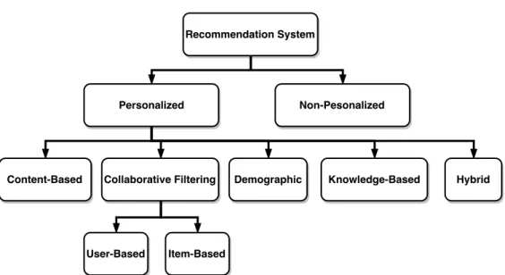
We can usually categorize recommendation algorithms into several types based on techniques, that produce a recommendation. According to [2], we will clas-sify Recommender Systems based on technique, that produce recommenda-tion. For clarity, the Figure 1.1 visualise the classificarecommenda-tion.

1.1.1.1 Personalized Recommendation System

This type of system leverages user’s past behavioral and based on it recom-mend desired items. Further, one can divide personalized systems into the following subcategories.

1.1.1.1.1 Content-based Filtering Content-based system is based on the analysis of the content of the items. It is intended to recommend items with a content similar to items, which the user enjoyed in the past or is looking at in the present. These type of recommenders are often based on creating a user profile, which stores user’s preferences, taste, and features of items [1].

1.1.1.1.2 Collaborative Filtering Collaborating filtering approaches can

be divided into two types: user-based CF and item-based CF. Both approaches are based on social interactions. The advantage of these types is that they do not need to extract any feature from items. Furthermore, they are able to recommend any items, even items with content, which does not correspond to any of the previous items that the user liked. User-based CF suggests rec-ommendation based on considering users having similar interest. Unlike the user-based collaborative filtering, the item-based CF looks for items similar to items user already rated. The crucial part of the algorithm is how the similarity is computed. From the collaborative point of view, two items are similar if the users agree about ratings [1].

Generally, CF-based models cannot deal with a new user or an item, be-cause they require a history of ratings of the user or the item to calculate the similarities, for the determination of the neighborhood. This issue is called cold start problem [3].

1.1.1.1.3 Knowledge-based This type of system is used in specific

do-mains, where the interaction history is very sparse or does not play a significant role. In this type of system, the algorithm considers the knowledge about the item and its features, user taste (asked explicitly), and various recommenda-tion criteria before providing the recommendarecommenda-tion [2].

1.1.1.1.4 Hybrid-based Hybrid recommender systems combine two or

more recommendation techniques to obtain better performance and mitigate drawbacks of any individual technique [4].

1.1.1.1.5 Demographic This technique is a recommendation based on

the knowledge of demographic data about the user, such as age, gender, em-ployment status, location and so on. The recommendation exploits demo-graphic similarities among users [2].

1.1.1.2 Non-Personalized

Non-Personalized recommender system does not incorporate the personal pref-erences of the user. All recommendations are identical, regardless on the user [5].

1.2. Recommendation Algorithms

Figure 1.1: Recommender System Classification

1.2

Recommendation Algorithms

This section covers several recommendation algorithms. The first part is ded-icated to traditional recommendation algorithms and the second part intro-duces models that incorporate deep learning techniques.

1.2.1 Traditional Recommendation Algorithms

This section cover two types of algorithms. One is memory-based algorithm, which tries to identifying the neighbors of user or item and the remaining two are model-based algorithm, which belongs to family of latent factors models.

1.2.1.1 Memory-based Collaborative Filtering Techniques

Memory-based CF algorithms use the entire set or a sample of the user-item interactions. It is assumed, that each user is part of a group of people with sim-ilar taste. By identifying the neighbors of the user, a prediction of preferences on new items is served. The most common representative are neighborhood-based CF algorithms. This type of CF algorithm uses the following steps [6]:

• calculate the similarity or weightwi,j between two users or two items, • serve a suggestion for the active user by taking the weighted average of

1.2.1.1.1 Neighborhood-based Algorithm Similarity computation be-tween items or users is a critical step. In case of item-based CF algorithm, the basic idea is to compute the similarity of all pairs of items. A similarity or weightwi,j between two items is calculated by taking the ratings of the users

who have rated both of the items and then applying a similarity measure. The prediction is then computed by taking a weighted average (for example equation 1.1) of the target user’s ratingsr on these similar items. User-based CF algorithm first calculates the similaritywu,v, between users u and v who

have both rated the same items [6].

pu,i = P n∈Nru,n−wi,n P n∈N|wi,n| (1.1) There are many different methods to calculate similarity or weight between users or items. Usual measures are for example correlation-based similarity (Eq. 1.2), cosine-based similarity (Eq. 1.3) and so on [6].

wu,v = P i∈I(ru,i−rˆu)(rv,i−rˆv) r P i∈I(ru,i−rˆu)2 q P i∈I(rv,i−rˆv)2 (1.2) wi,j = ~i·~j k~ikk~jk (1.3)

1.2.1.1.2 Scalability Complexity of the neareset neighbor algorithm grows

with both the number of users and the number of items, hence it has limited scalability for large datasets. From view of interactions dynamic, user-based CF suffers more than item-based CF. Unlike similarity between users, items similarity is more or less static, therefore it enables precomputing of item-item similarity [7].

1.2.1.2 Matrix Factorization

Matrix Factorization algorithm belongs to a family of latent factors model. Latent factor model tries to explain the ratings by characterizing both user and item by a vector inferred from the ratings pattern. When user and item do highly correspond, it provides a lead to a recommendation.

Matrix Factorization models map users and items to a joint latent factors

f dimensional space. User-item interaction are modeled as inner products in that space. Each user is then represented by vector~u∈ Rf _{and each item by}

vector~v ∈ Rf_{. The dot product~u}T

u~vi captures the interactions between user

u and itemi[8]. This approximates rating given by user uto item i:

1.2. Recommendation Algorithms

The most challenging part is finding the mapping of each item and user to factor vectors uu, vi ∈ Rf. However, when the mapping is complete,

recom-mender system can easily estimate unobserved ratings by using the equation 1.4.

A common way to learn the factor vectors uu and vi is to minimize the

regularized squared error on the set of observed and unobserved ratings 1.5. min

u∗_,v∗

X

(u,i)∈K

cu,i(ru,i−uTuvi)2+λ(kuuk2+kvuk2) (1.5)

Here, K is the set of the all (u, i) pairs, the constant λcontrols the extent of regularization and cu,i is confidence of rating [9].

1.2.1.2.1 Learning Procedures Several learning algorithms have been

developed for searching the minimum of 1.5. The most common ones are stochastic gradient descent, alternating least squares and coordinate descent.

1.2.1.2.1.1 Stochastic Gradient Descent The algorithm loops through

all ratings in the training set, for each training example compute associated erroreu,i =ru,i−uTuvi. Then update parameters according to Eq. 1.6.

uu=uu+γ·(cu,ieu,i·vi−λuu)

vi =vi+γ·(cu,ieu,i·uu−λvi)

(1.6)

1.2.1.2.1.2 Alternating Least Square The ALS technique is based

on switching between fixeduuand fixedvi. When alluare fixed the

optimiza-tion problem becomes quadratic and can be solved optimally. Then system recomputesviby solving a least squares problem (in general e.g. 1.7) and vice

versa [8].

θ= (XTCX)−1XTCY (1.7) In general, stochastic gradient descent is easier and faster than ALS, how-ever ALS can be easily parallelized. The algorithm computes each uu and

vi independently of the other users, items factors respectively. Due to this

independence, computation can be massively distributed [8].

1.2.1.2.1.3 Coordinate Descent Approaches The basic idea of

co-ordinate descent is similar to ALS. A single variable is updated at a time while keeping others fixed [10].

1.2.1.2.1.4 Extensions In recent years, lots of extensions have been

developed, for example adding user, item, and global biases. The prediction of the rating is then decomposed to 4 parts µ,bi,bu and uTuvi 1.8, whereµ is

the overall average rating, and the parametersbu and biindicate the observed

deviation of useruand itemi, respectively, from the average. Further, adding user and item bias terms tend to capture much of the observed signal, their accurate modeling is vital. Hence, this allows each component to explain only the part of a signal relevant to it [8].

Another example is temporal dynamics, which enriched the static model with the ability to model temporal effects [8]. The termsbt

i,btu and utuTvt_i can

then vary over time 1.9. ˆ

ru,i=µ+bi+bu+uTuvi (1.8)

ˆ

rt_u,i=µt+bt_i+bt_u+ut_uTvt_i (1.9)

1.2.1.2.1.5 Scalability The time complexity per iteration of SGD is

O(|K|k), ALSO(|K|k2+ (m+n)k3) and coordinate descent based algorithm (CCD++)O(|K|k), whereK is the set all observed ratings,m is the number of users, n the number of items, and k the number of factors (size of latent vector representation). Despite the fact, that ALS has the worst asymptotic complexity, massive parallelization can mitigate this issue. Further, the SGD suffers from sensitivity on the choice of the learning rate, when compared to CCD++[11].

1.2.1.3 Factorization Machines

The Factorization Machines is another example of factorization models sim-ilarly to MF. It combines the advantages of Support Vector Machines with factorization models. FMs model interactions between variables using factor-ized parameters. Thanks, this property, FMs are capable estimate interaction even in a problem with huge sparsity where other models fail [12]. Equation 1.10 shows factorization machine of degreed= 2.

ˆ y(~x) =w0+ n X i=1 wixi+ n X i=1 n X j=i+1 < vi, vj > xixj (1.10)

where~x is vector of features,w0 is global bias, wi models the strength of i-th

feature, vi and vj are latent representations of feature xi and xj, < vi, vj >

is dot product and model interactions between the i-th and j-th feature. The FM can be extended to arbitrary degree of interaction.

1.2.1.3.1 Learning Procedure The author proposed several learning

procedures such as stochastic gradient descent, alternating least squares, and Markov Chain Monte Carlo. Even stochastic gradient descent can learned

1.2. Recommendation Algorithms

parameters efficiently. The gradient of the FM model is [12]:

∂ ∂θyˆ(~x) =        1, ifθ isw0 xi, ifθ iswi xiPnj=1vj,fxj −vi,fx2i, ifθ isvi,f (1.11)

1.2.1.3.2 Scalability The model equation 1.10 is feasible to compute in

linear time O(kn), where n is a number of features and k size of latent rep-resentation. Thus, the algorithm does not suffer from pairwise interactions [12].

1.2.2 Deep Learning based Recommendation Algorithms

In many fields such as computer vision and speech recognition, deep learning (DL) is tremendously successful. This trend continues the past few decades and the academia and industry have been in a race to apply deep learning to a wider range of application. Recently, deep learning has been appearing in the domain of recommendation systems and brings more opportunities in rein-venting the user experiences for better customer satisfaction. Deep learning can efficiently capture the nonlinear and non-trivial user-item relationships and leverage abundant data sources such as contextual, textual and visual information [13].

1.2.2.1 Deep Learning Techniques

This part will briefly introduce deep learning techniques, which are used in following recommender system algorithms.

1.2.2.1.1 Multilayer Perceptron Multilayer Perceptron is a feedforward

neural network with multiple (one or more) hidden layers between input layer and output layer. The perceptron can hold arbitrary activation function.

1.2.2.1.2 Autoencoder Autoencoder is an unsupervised model, which is

trained to reconstruct its input data in the output layer.

1.2.2.1.3 Recurrent Neural Network Recurrent Neural Network has

been designed to be able model sequential data. In RNN are loops and mem-ories to remember previous computations. Variants such as Long Short Term Memory (LSTM )and Gated Recurrent Unit (GRU) have been developed to improve network capabilities.

1.2.2.2 Collaborative Deep Learning

Collaborative Deep Learning is a hierarchical Bayesian model, which jointly models deep representation for the content information and collaborative fil-tering for the ratings matrix. The model combines stacked denoising autoen-coder (SDAE) with probabilistic matrix factorization. SDAE is a deep neural network, which is able to process various side information. PMF acts as the task-specific component. These two parts are tightly coupled and enable CDL to balance the influences of side information (SDAE) and ratings (PMF) [13]. The generative process can be defined as follow:

• For each layer l of the SDAE network,

– For each columnnof weight matrixWl, drawWl,∗n∼ N(0, λ−w1IDl).

– Draw the bias vector bl∼ N(0, λ−w1IDl)

– For each rowiof Xl,i∗ ∼ N(σ(Xl−1,i∗Wl+bl), λ−s1IDl)

• For each layer itemi,

– Draw a clean inputXc,i∗∼ N(XL,i∗, λ−n1IIi)

– Draw a latent offset vector i ∼ N(0, λ−u1ID) and set the latent

item vector: Vi =i+XTL

2,i∗

• Draw a latent user vector for each useru,uu ∼ N(0, λ−u1, ID)

• Draw a ratingru,i for each user-item pair (u, i), ru,i ∼ N(uTuvi, Cu,i−1)

where Wl and bl arethe weight matrix and biases vector for layer l, Xl

rep-resents layer l. λw, λs, λn, λv, λu, are hyper-parameters, Cu,i is a confidence

parameter for measuring the confidence to observation,Xcis the clean input,

X0 is corupted input [13].

Several technique to find parameters of model may be applied. The authors expoited an EM-style algorithm for obtaining the maximum a posteriori es-timates. In this case, one maximizes join-log-likelihood of U, V, Xl, Xc, Wl, bl,

and R given λw, λs, λn, λv, λu. Then, equation 1.12 can give intuition behind

the model. L=−λu 2 X u kuuk2− λw 2 X l∈layers (kWlk2+kblk2) −λv 2 X j kvj−XTL 2,j∗ k2−λn 2 X j kXL,j∗−Xc,j∗k2 −λs 2 X l X j kσ(Xl−1,j∗Wl+bl)−Xl,j∗k2 −X u,i Cu,i 2 (ru,i−u T uvi)2. (1.12)

1.2. Recommendation Algorithms

If λs goes to infinity, it simplifies model and the likelihood reduces to 1.13: L=−λu 2 X u kuuk2− λw 2 X l∈layers (kWlk2+kblk2) −λv 2 X j kvj−fe(Xs,j∗, W+)Tk2− λn 2 X j kfr(Xs,j∗, W+)−Xc,jk2 −X (u,i) Cu,i 2 (ru,i−u T uvi)2 (1.13) whereW+ denotes the collection of all layers weights and biases,fe(·, W+) is

encoder function andfr(·, W+) computes encoding and then reconstructs the

content vector of item j. The first two terms are regularization, second line terms balance model reconstruction error between item content vector Xc,j

and item latent vector vj and the last term incorporate task-specific

compo-nent. One can approximate the prediction rating as 1.14 for both models.

Ri,j ≈uTi vj (1.14)

1.2.2.2.1 Learning Procedure One of the possible learning procedure is

very similar to the idea of ALS. Learning algorithm alternates between fixed

W+ and latent representations U, V of users, items, respectively. Latent representations updates (Equations 1.15) lead to the updates rules similar to 1.2.1.2.1.2 and for W and b, authors use a modified version of backpropagation [13].

uu = (VTCuV +λuIk)−1VTCuRu

vi= (UTCiU +λiIk)−1(UTCiRi+λvfe(X0,j∗, W+))

(1.15)

1.2.2.2.2 Scalability Authors presented update rules have the

computa-tional complexity of updating ui (O(k2J +k3)), where k is the size of

la-tent representation and J is the number of items. Updatevj has complexity

O(k2I+k3+SK1), whereI is the number of users, S is the size of the

vocab-ulary, and K1 is dimensionality of output in the first layer.

1.2.2.3 Wide & Deep

This general model can be used for both regression and classification problems. The wide part of the model is single layer perceptron, and the deep learning part is multilayer perceptron. The authors suggested that combining these two components enable to capture both memorization and generalization. For catching the direct features from historical data is proposed the memorization component and deep learning component produce more general and abstract representation [13].

Formally, the wide component is a generalized linear model 1.17, where x

is the vector of features,w and bare model parameters. The features include various transformed and raw features. The authors noted, that cross-product transformation is one of the most important [14].

y=wTx+b (1.16)

The deep component is a feed-forward neural network. Categorical features are first transformated to low-dimensional and dense real-valued vectors of-ten referred as an embeddings. At the start, the embeddings are initialized randomly and during model training are updated to minimize the final loss function. These embeddings are then fed into the hidden layers. Each hidden layer calculates the following computation:

a(l+1)=f(W(l)a(l)+b(l)) (1.17)

wherel is the layer number,f is the activation function anda(l), b(l) andW(l)

are the activations, bias, and weights at l-th layer.

1.2.2.3.1 Learning Procedure The wide component and deep

compo-nent are coupled using a weighted sum of their outputs and then fed into one common logistic loss function for joint training. Thus, during training both components are trained simultaneously. The authors suggested using backpropagation for training[14].

1.2.2.3.2 Scalability The authors have evaluated the Wide & Deep model

on a massive-scale commeracial app store Google Play. At the peak, the model has had to score over 10 million apps per second [14].

1.2.2.4 Session-based GRU4Rec

GRU4Rec is significantly differ from models mentioned before. The task of previous models is simply recommend the most relevant items to user, whereas the goal of GRU4Rec is recommend item based on user session. The authors argue, that this approach is more suitable for many e-commerce recommender systems. Particularly small retailers, most of news and media sites, because they do not typically track the user-id’s of the users that visit their sites over a long period of time. Further, cookies and browser fingerprinting are not always reliable enough [15].

To overcome this issue, authors have proposed GRU-based reccurent neural network (RNN). The current state of session is fed to the RNN while the output of is the item of the next event in the session. The state of the session is either the item of the current event or the events in the session so far. The authors have used 1-of-N encoding in the first case, i.e. binary vector equal

1.2. Recommendation Algorithms

to the number of items filled with zeros except the coordinate corresponding to the active item and weighted sum of theses representations [15].

The architecture is composed from GRU layer(s) and additionaly feedfor-ward layers can be added between the last and the output layer. The output layer predicted preferences of the items of being the next in the session. When more then one GRU layers are used, the hidden state of the previous layer is the input of the next one. Further, optionally, the input can be connected to the successive GRU layers. The authors has reported, that this option improves performance [15].

1.2.2.4.1 Learning Procedure The authors proposed a session-parallel

mini-batches, a sampling method for output and own loss function. Mini-batches have been constructed as follow:

• create ordered sessions,

• use first event of the first X sessions to form input, desired outputs are the seconds events of active session,

• the next mini-batch is formed from the seconds events and so on,

• if any session end, the next available session is put in its place.

The loss function 1.18 belongs to family of ranking losses and measure relative rank of the relevant item according to sampled items. Ns is sample

size, σ is a sigmoid function, ˆr are predicted item scores.

Ls= 1 Ns Ns X j=1 σ(ˆrs,j−rˆs,i) +σ(ˆr2s,j) (1.18)

Due to a potentially large number of items, computing scores for each of them would be unusable in practice. Therefore the authors have suggested sam-pling items in proportion to their popularity. Instead of generating separate samples, they have been used items from previous mini-batches as negative examples [15].

1.2.2.4.2 Scalability The authors have suggested a method for

signifi-cantly reducing time complexity. However, the authors in [16] argue, that much more simple methods as frequent-pattern-based approaches can be com-petitive in accuracy and result strongly depends on datasets characteristics. Compare to GRU4Rec these simple models learn much faster and applying the rules is very fast. Despite this fact, the authors expect that continuously improved RNN-based methods will be able to outperform the frequent pattern based algorithms used in their evaluations [16].

1.3

Hyper-parameters Optimization Techniques

In the context of a recommender system, hyper-parameters optimization is essential for adequate performance in real-world applications. For example, on the recommender system related ads recommendation, authors reported results, which thanks online tuning of algorithm showed a significant 4.3 % revenue lift overall traffic [17].

An offline-world fine-tuning is as essential as fine-tuning in a real-world running application. Deploying low-performance models can lead to decreas-ing revenue, user’s satisfaction, a number of users, etc. Therefore is necessary do a careful model preselections.

Most of the recommender algorithms have numerous hyper-parameters, which can be tuned and accordingly significantly change their behavior. To deal with optimization of high number and ill-conditioned hyper-parameters has developed several techniques and different approaches.

1.3.1 Problem Definition

Most of machine learning task can be described as training model M which minimizes some predefined loss functionsL(Xtest;M) on given test dataXtest. The model M is constructed by a learning algorithm A using a training set

Xtrain. The algorithm A can be parametrized by hyper-parameters H itself,

e.g. M =A(Xtrain, H). The goal of hyper-parameters search is to find a set of hyper-parametersH of modelM that yield to minimize functionL(Xtest, M) [18]. Formally:

H∗= arg min

H

L(Xtest;A(Xtrain;H)) (1.19)

1.3.2 Hyper-parameter Optimization Techniques

This section provides a brief overview of optimization techniques that have been reported in recent years in the domain of recommendation systems.

1.3.2.1 Grid Search

Grid search is a method, which calculates all possible hyper-parameters set-tings. It works only with discrete hyper-parameters since the continuous hyper-parameters space is infinite. Therefore is often necessary discretize continuous hyper-parameters. Recommendations algorithms have often sev-eral hyper-parameters and then is grid search highly inefficient, due to the exponential growth of possible combinations of hyper-parameters.

1.3.2.2 Random Search

Random search uniformly samples hyper-parameters within given bounds. De-spite this simplicity, the random search has huge advantage in easy

paralleliza-1.3. Hyper-parameters Optimization Techniques

tion.

1.3.2.3 Greedy Search

Gready search optimize only one hyper-parameter a time, while fixing re-maining hyper-parameters. For each hyper-parameter is selected m random samples and then fixated to the best from the random samples. The procedure is then repeated with remaining hyper-parameters.

1.3.2.4 Random Walk

Random Walk is an iterative method. In each step, it computes the perfor-mance of each neighbour, based on a selection mechanism select one of the neighbours and makes step towards this neighbour.

1.3.2.5 Simulated Annealing

Simulated Annealing is related to the random walk method. It uses tempera-ture as a control variable that manages probability of selection worse solutions than the current one by selection mechanism. As temperature decrease, the probability of choosing worse solution also decrease.

1.3.2.6 Nelder-Mead

Nelder-Mead method search minimum of function by spanning a simplex in the hyper-parameter space. The simplex hask+ 1 vertices, wherekis the number of hyper-parameters. The simplex can move in space of hyper-parameters by leveraging four transformation: reflection, contraction, expansion and shrink-ing [19].

1.3.2.7 Particle Swarm Optimization

Particle swarm optimization is inspired by behaviours of swarms. A popu-lation of particles called swarm move in the space of hyper-parameters and maintains its velocity and its best position. The entire swarm store the global best position. Each particle adjust its position according to personal and global best position.

1.3.2.8 Genetic Algorithm

Genetic algorithm is inspired by the process of natural selection present in evolution. Each individual is part of a population and it is a candidate for a solution. The information about the individual is encoded to an array. The following process of optimization is iterative. In each round, the individuals are combined, possibly mutated and selected based on a fitness function. Only

those individuals with high fitness are likely to transfer their information to the next generation.

1.3.2.9 Sequential Model-based Optimization

Model-based optimization methods build a regression model that predicts the performance of a target algorithm. These models iterate between the addi-tional data collection and constructing approximation model, often called sur-face or surrogate model. The model is fitted to a training set (θ1, y1), . . .(θn, yn)

of observed performanceyi when target algorithm run with hyper-parameters

Chapter

2

Solution Analysis

2.1

Algorithms Analysis

The goal of selected algorithms is to be able to operate with various datasets without expert knowledge about the content of these datasets. The datasets contain a huge number of interactions and items related auxiliary informa-tion. MF algorithm is one of the most successful algorithms in domain of recommendation systems which for training leverage only user-item interac-tions [21]. In contrast with MF, CDL algorithm is capable use various kind of auxiliary information and therefore, in some cases, increase recommendation quality. For these reasons, MF and CDL have been chosen.

2.1.1 Matrix Factorization

From wide family of matrix factorization based algorithms [22], the algorithm in [23] has been mainly followed because of stability of learning algorithm and parallelization potencial. Further, it is extended by optional user and item bias terms.

The system learns by minimizing the squared error function: min u∗_,v∗ X ru,i∈observed (1 +α)(ru,i−rˆu,i)2+ X ru,i∈missing (0−ˆru,i)2 +X u λnukuuk2+ X i λnikvik2 (2.1)

where ˆru,i is bu+bi+uuTvi, bi and bu are bias terms for user u respectively

item i, ru,i is observed rating given user u to item i, uu and vi are user u

respectively item i latent vectors, term 1 +α plays a role of weight, nu and

ni are numbers of observed ratings for user u respectively item i and λ is

regularization parameter.

To deal with a searching minimum of function 2.1 one can use several techniques as we have discussed earlier in section 1.2.1.2. The Weighted

Al-ternating Least Square optimization method has been used in this work. The solution of the Least square problem is obtained by solving a system of linear equations a.k.a normal equation [24]. Following pseudocode describes algo-rithm without biases [23]:

1 initialize V, U; 2 for i toN do 3 U tU ←UTU

4 foreach i ∈items do

5 U tU ← UtU +αU_obsT U_obs+λn_iI; 6 U tr ←(1 +α)Uobsrobs;

7 Vi ←solve(U tU, U trobs);

8 end 9 V tV ←VTV 10 foreach u∈ users do 11 V tV ←V tV +αV_obsT Vobs+λnuI; 12 V tr ←(1 +α)V_obsr_obs; 13 U_u←solve(V tV, V tr_obs); 14 end 15 end

Algorithm 1:Weighted ALS Matrix Factorization

I in 1 refers to identity matrix,VobsandUobsto latent factors corresponded

to observed user-items interactions.

Matrix factorization with biases (Algorithm 2) has almost identical pseu-docode except that it is necessary to subtract biases from ratings, add dummy columns filled with value one and then do carefully indexing during optimiza-tions. Superscript(1)expresses added dummy columns, (:,:) indexing matrices and I0 _{resp. I}

2.1. Algorithms Analysis element. 1 initializeV(1),U(1); 2 fori to N do 3 U tU ←U(1)(:,:−1)TU(1)(:,:−1) 4 foreachi ∈ items do 5 U_obs ←U_obs(1)(:−1) 6 bu ←U_obs(1)(−1)

7 U tU ← UtU +αU_obsT U_obs+λniI0; 8 U tr←(1 +α)U_obs(r_obs−b_u);

9 Vi(:−1)←solve(U tU, U trobs);

10 end 11 V tV ←V(1)(:,1 :)TV(1)(:,1 :) 12 foreachu ∈ usersdo 13 V_obs←V_obs(1)(1 :) 14 b_v ←V_obs(1)(0) 15 V tV ←V tV +αV_obsT V_obs+λn_uI₀; 16 V tr←(1 +α)Vobs(robs−bv); 17 U_u(1 :)←solve(V tV, V tr_obs); 18 end 19 end

Algorithm 2:Weighted ALS Matrix Factorization with biases

2.1.2 Collaborative Deep Learning

Simplified version of CDL [25] with minor change has been used in this work. That change incorporates adjusting each user’s latent vector regularization to

λu multiply by his number of ratings.

The simplified version was presented as part of the KDD 2016 [26]. Hence, that version is possible to separate into two components, i.e., autoencoder and Matrix Factorization and one can recycle the implementation of the matrix factorization 2.1.1 with just minor adjustments.

The system learns by minimizing the following function [27]: min u∗_,v∗_,W∗_,b∗ X ru,i∈observed (1 +α)(ru,i−rˆu,i)2+ X ru,i∈missing (0−rˆu,i)2 +λunu X u kuuk2 +λw X l∈layers (kWlk2+kblk2) +λv X j kvj−fe(Xs,j, W+)Tk2 +λn X j kfr(Xs,j, W+)−Xc,jk2 (2.2)

whereW and bare autoencoder’s weights and biases,Xs,j is vector of item j

content,Xc,j is vector of reconstructed itemj content,vj is the item j latent

representation comming from the Matrix Factorization component, fe is the

encoder function andfris function returned the reconstructed content vector.

The first line of equation refers to matrix factorization component, the second line is user’s regularization term, the third line is autoencoder’s weights and biases, the fourth line forces item’s latent vectors and item’s encoded representation to be similar in Frobenius norm and the last line do the same with original and reconstructed item’s content.

The pseudocode 3 describes learning procedure of simplified CDL. One can see, that the autoencoder component and the matrix factorization component are not trained jointly, but alternating between each other. While parameters one of the components have been training, parameters second component are

2.2. Optimization Procedure

fixed.

1 initialize V, U;

2 preprocess content of items; 3 fori to N do

4 foreach(X_batch, V_batch)∈batches do

5 trainAutoEncoder(X_batch, V_batch);

6 end

7 theta←AutoEncoder(X);

8 U tU ←UTU;

9 foreachi ∈ items do

10 U tU ← UtU +αU_obsT U_obs+λvI;

11 U tr←(1 +α)U_obsr_obs+λ_vtheta_i;

12 Vi←solve(U tU, U trobs);

13 end 14 V tV ←VTV; 15 foreachu ∈ usersdo 16 V tV ←V tV +αV_obsT V_obs+λ_uI; 17 V tr←(1 +α)Vobsrobs; 18 U_u ←solve(V tV, V tr_obs); 19 end 20 end

Algorithm 3:Collaborative Deep Learning

2.1.3 User Recommendation Calculation

Conventional approach to user recommendation computation is for each item to calculate score as dot product (equation 2.3) between latent user repre-sentation and latent item’s reprerepre-sentation and then sort them in descending order. On the top of the list are the most relevant items to the user.

score(u, v) =u·v=

n

X

i=1

uivi =u1v1+u2v2+· · ·+unvn (2.3)

Second approach tested in this work is compute the score as a cosine similarity between user u and itemv 2.4.

score(u, v) =cos(u, v) = u·v kukkvk = Pn i=1uivi q Pn i=1u2i Pn i=1vi2 (2.4)

2.2

Optimization Procedure

Probably the most relevant source to this thesis is the work [21]. Authors benchmarked various algorithms on four real-world datasets. The algorithm

chosen for hyper-parameter optimization was the matrix factorization with the objective to optimize the RMSE (root mean square error). As the con-clusion, the authors suggested that in scenarios, where marginal improvement plays the critical role the Nelder-Mead algorithm should be used. The algo-rithm achieved the best performance on all datasets, followed by simulated annealing. Although Nelder-Mead algorithm achieved the best performance, improvement compared to random search was neglectful. Therefore after con-sidering many advantages of random search, such as full parallelization, sim-plicity, constant and nearly negligible computation time, they recommend use it for hyper-parameter optimization in the domain of recommender systems.

Authors in [28] demonstrated on state-of-the-art ANN models for dialog act classification, that optimizing hyper-parameters using Gaussian Processes (GP) further improves the results and reduces the computational time by a factor of 4 compared to a random search. Further they compared various GP settings and impact of the number of initial random hyper-parameter combinations.

Based on these results, Gaussian Processes and Random Search methods have been chosen as algorithms suitable for fine-tuning recommendation algo-rithms.

2.2.1 Evaluation Measures

As in [27] we have adopted recall as a measure of recommender algorithm accuracy. We sort the predicted ratings of the candidate items and recommend the top K items to the target user. Equation 2.5 show recall calculation. The final result reported is the average recall over all users.

recall@K ← #Lrec

min(K,#L) (2.5)

where #Lrec is number of items that the user likes among the top K, #L is

total number of items that the user likes.

As an additional measure, catalog coverage has ben chosen. Catalog cov-erage can be express as the percentage of the available items which effectively are ever recommended to a user[29]. It is given by equation 2.6:

coverage@K ← S u∈test users Iu |I| (2.6)

whereIu is a set of recommended items to user during evaluation phase and

I is set of all items in catalog.

2.2.2 Optimization Procedure Design

At first, it is necessary to identify hyper-parameters suitable for fine tun-ing. This is done by initial Random Search (RS). Based on results of the

2.2. Optimization Procedure

initial random search, part of hyper-parameters let be fixed and remaining hyper-parameters are searched by grid search to expose simple and obvious dependencies between hyparameters and algorithm performance. The per-formance of an algorithm is measured by recall desribed in 2.2.1.

After detecting obvious dependencies between hyper-parameters and al-gorithm performance, a selected subset of hyper-parameters is fixed or set to an appropriate range and remaining hyper-parameters are tuned according to GP or RS. Algorithm 4 is an overview of the process.

input :D(dataset), A (recommendation algorithm),O (either GP or

RS),RS (Random Search), H (space of Ahyper-parameters)

1 res←{}; 2 fori to N do

3 θ← selecthyper-parameters(RS,A,H);

4 model ← train(A,θ ,D_train);

5 res← eval(model,Dtest); 6 end

7 H ← adjust(H, eval(res)); 8 res← {};

9 fori to M do

10 θ← selecthyper-parameters(O,A,H);

11 model ← train(A,θ ,D_train);

12 res← eval(model,D_test); 13 end

14 eval(res);

Algorithm 4:Evaluation procedure

Further, due to strong relationship between MF and CDL, second approach has been designed. CDL and MF have broad intersection of hyper-parameters. Therefore, one can try to leverage the knowledge gained from MF optimiza-tion and set CDL parameters to the same values as associated hyper-parameters of the optimal MF model. Algorithm 5 shows an overview of the

process.

input :D(dataset), A (CDL algorithm), O (either GP or RS), HM F

(MF optimal hyper-parameters),HCDL (space of CDL

hyper-parameters)

1 H_CDL ← adjust(H_CDL,H_{M F}); 2 res← {};

3 fori to M do

4 θ ←selecthyper-parameters(O,A,H_CDL);

5 model ← train(A,θ ,D_train);

6 res ←eval(model,Dtest); 7 end

8 eval(res);

Chapter

3

Realization

Within the scope of this thesis, a dataset preprocessing pipeline, a recom-mender algorithm evaluation pipeline, a hyper-parameter fine-tuning pipeline and two algorithms have been implemented. During implementation, we have focused on scalability and a potential possibility to deploy particular algorithm as a component of the real-world hybrid recommender system.

3.1

Programming Language

The whole system is written in Python focusing on easy extensibility and editability. The main reason for choosing Python as a programming language is that it enables fast prototyping of an idea [30]. Also, Python contains an enormous amount of machine learning libraries.

3.2

Library Usage

Following libraries has been used in this work.

• NumPy 1 – NumPy is a fundamental package for scientific computing with Python.

• PyTorch2_{– PyTorch is a popular deep learning framework with pythonic}

syntax.

• Spark 3 – Apache Spark is a powerful open source processing engine built around speed, ease of use, and sophisticated analytics4.

1_{http://www.numpy.org/} 2 http://pytorch.org/ 3 http://spark.apache.org/docs/2.1.0/api/python/pyspark.html 4 https://databricks.com/spark/about

• Scikit-optimize5– Scikit-optimize (skopt) is a simple and efficient library to minimize (very) expensive and noisy black-box functions.

• Scikit-learn 6 – Scikit-learn provides simple and efficient tools for data mining and data analysis.

• Matplotlib 7 _{– Matplotlib is a Python 2D plotting library which}

pro-duces publication quality figures in a variety of hardcopy formats and interactive environments across platforms.

• Pandas8 – Pandas is an open source library providing high-performance, easy-to-use data structures and data analysis tools for the Python pro-gramming language.

• Majka 9 – Majka is a free morphological analyzer. Majka includes databases for Czech, Slovak, Polish, Swedish, German, French, Italian, English, Portuguese and others.

• TensorFlow10 – TensorFlow is mainly designed for deep neural network models.

• Jupyter 11 – Jupyter Notebook is an open-source web application that allows create and share documents that contain live code, equations, visualizations and narrative text.

3.3

Implementation

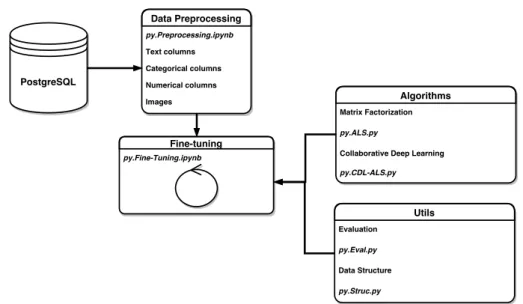
The diagram 3.1 provides an overview of the whole system, each component is then described in following sections.

3.3.1 Data Access

nonpublic datasets (described in 4.1) were provided in the PostgreSQL database. The Spark Python API (PySpark)12was used to connect to the database and basic filtering operations. The main advantage of this approach is that PyS-park allows multicore data processing. After data loading and basic filtering, PySpark data structures have been transformated to Pandas data structure for easier manipulation.

5_{https://scikit-optimize.github.io/} 6 http://scikit-learn.org/stable/ 7_{https://matplotlib.org/} 8 https://pandas.pydata.org/ 9_{https://nlp.fi.muni.cz/czech-morphology-analyser/} 10 https://www.tensorflow.org/get˙started/ 11 http://jupyter.org/ 12 http://spark.apache.org/docs/2.1.0/api/python/pyspark.html

3.3. Implementation

Figure 3.1: System Overview

3.3.2 Data Preprocessing

Despite the fact that this work has focused on minimizing the need to incorpo-rate data analysis and the expertise of datasets owners, some pre-processing of datasets has been required. At the end of preprocessing serialized data has been stored in disk.

3.3.2.1 Numeric Data Preprocessing

Numerical columns have been transformed according to the formula 3.1, where

cindicated column, vc

i original value in row of columnc, ˆµcis mean and ˆσc is

standard deviation of values in particular column and ˆv_ictransformated value

v_ic. ˆ vc_i ← v c i −µˆc ˆ σc (3.1)

3.3.2.2 Categorical Data Preprocessing

Rows with categorical data (e.g. tags, categories) have been simply split by appropriate separator.

3.3.2.3 Text Preprocessing

In cases, when columns contain text in natural language, for instance, news article description or title, a lemmatizer has been used. In the scope of this work, datasets suitable for this type of processing have been only in the Czech language. The data processing steps for each row have been as follows:

• removing punctuation,

• removing stopwords (the lists of Czech stopwords 13and 14),

• collecting the first lemma suggested by Majka,

• chaining collected lemmas.

3.3.2.4 Image Preprocessing

For image preprocessing has been used script available in GitHub 15. The script is a wrapper for feature extraction in TensorFlow. It offers well known pre-trained models on ImageNet 16. From offered models, the Inception v4 has been selected cause reported high performance compared to other mod-els. Further, the script allows choosing the extraction layer that returns the resulting embeddings. The Logits layer has been chosen.

Because the datasets do not contain images but only links to images, the first step has been downloading images to disk and then using the script for feature extraction mentioned above. To summarize, whole procedure has been looked as follows:

• collecting all links to images,

• using the linux command wget to download images to disk,

• using the script to extract features from images.

After image feature extraction, each one has been described as vector of size 1001 with real numbers.

3.3.2.5 Leveraging Preprocessed Data

After data has been preprocessed, categorical columns and lemmatized text data have been chained and transformed to a vector with parameterizable size by function HashingVectorizer17.

HashingVectorizer function turns a collection of text documents into a matrix holding token occurrence counts (or binary occurrence information). It allows normalizing token frequencies, either l1 norm or projected on the euclidean unit sphere. The HashingVectorizer implementation leverages the hashing trick to find the token string name to feature integer index mapping. Hashed data has been then chained with numerical columns. This ap-proach is universal and it is possible to replicate on an arbitrary dataset.

13 https://github.com/stopwords-iso/stopwords-cs 14 https://github.com/crodas/TextRank/blob/master/lib/TextRank/Stopword/czech-stopwords.txt 15_{https://github.com/tomrunia/TF˙FeatureExtraction} 16 https://github.com/tensorflow/models/tree/master/research/slim#pre-trained-models 17 http://scikit-learn.org/stable/modules/generated/sklearn.feature˙extraction.text.HashingVectorizer.html

3.3. Implementation

3.3.3 Algorithms

The following sections describe implementation details of chosen algorithms and bring some insight to implementation scalability. Simply put, the imple-mentation of Collaborative Deep Learning uses the impleimple-mentation of MF. Therefore MF results also apply to the MF component of CDL.

3.3.3.1 Matrix Factorization

As noted in the section 2.1.1, Weighted Alternative Least Squares approach with solving a normal equation has been used. This approach has one im-mediately visible advantage and one disadvantage. Because calculation of a user latent vector is independent to other users (same for items), calculations are easy to parallelize. This property is leveraged, for example, by the ML-lib ML-library (Apache Spark) 18. On the other hand, solving a system of linear equations is asymptotically cubic for a solver used in this work19.

The reason, why the official implementation has not been used, is that original version20 is implemented in C++ and MATLAB, therefore, it would be hard and expensive to incorporate it into the current hybrid recommender system. Further, due to a sequential implementation of simplified version 21, this version is not scalable and it is not feasible to use it for huge datasets.

3.3.3.1.1 Computation Parallelization Due to the global interpreter

locker (GIL)22_{, it is not feasible to use a thread-level parallelization for}

com-putations speed up. Therefore, Python package multiprocessing has been used

23 _{for a process-level parallelization. It allows distributing calculations of user}

and item latent representations to multiple processes.

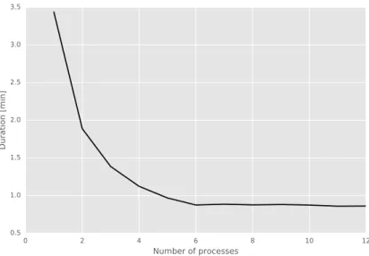
A new artifical dataset has been generated for measurements. The dataset contains approximately 1 million users, 100 thousand items and 10 millions interactions. Each measured parametrization has been repeated three times and reported best achieved wall time. For measurement, standard IPython function timeit 24 _{has been used. The calculations were run on a machine}

with 6 physical cores and 6 logical cores. More details are in appendix A.1.2. Fig. 3.2 shows speed up with respect to the number of processes. On the x-axis is number of processes used to compute latent representations and on the y-axis is duration in minutes. One can see, that duration decreases according to a number of physical cores. After the number of physical cores is exceeded, the time consumed by computation stays approximately the same.

18 https://spark.apache.org/docs/2.2.1/mllib-collaborative-filtering.html 19_{http://www.netlib.org/lapack/lug/node71.html} 20 https://github.com/js05212/CDL 21_{https://github.com/js05212/MXNet-for-CDL} 22 https://wiki.python.org/moin/GlobalInterpreterLock 23 https://docs.python.org/3.6/library/multiprocessing.html 24 http://ipython.readthedocs.io/en/stable/interactive/magics.html

0 2 4 6 8 10 12 Number of processes 0.5 1.0 1.5 2.0 2.5 3.0 3.5 Duration [min]

Figure 3.2: Scalability: number of processes

3.3.3.1.2 Data Structures To leverage process-level parallelization, it

has been necessary to choose an appropriate data structure for storing la-tent representations of users and items. For this purpose has been chosen a data structure multiprocessing.Array, which is offered by the same package as process-level parallelization. This structure allows to share memory between processes.

Furthermore, it has been shown it is very important to choose the right data structure for quick access to user and item data. Therefore, a new data structure has been implemented, which is fit to the MF implementation in this work. It is allows by fast indexing in Python list data structure access to data. One disadvantage is that for users and items, the structures have to be created separately, so it claims twice as much memory, but on present hardware, this is not restrictive.

3.3.3.1.3 Latent Representation Calculation For linear algebraic

op-erations necessary for computation latent representations, the package NumPy has been used. To get maximal performance, disabling multithreading support in NumPy package has been necessary.

In the Figure 3.3 one can see a relation between the size of latent repre-sentation and the duration of calculation. As before, each measurement has been repeated three times and reported the best-achieved wall time. One can see exponentially increasing duration with respect to the size of latent representation.

3.3. Implementation

0 100 200 300 400 500 Length of latent representation

0 5 10 15 20 25 Duration [min]

Figure 3.3: Scalability: size of latent representation

3.3.3.2 Deep Collaborative Filtering

As noted before, one component of CDL is the adjusted MF implementation. This modification does not change the complexity of MF implementation. Therefore in the following part, we will focus more on an Autoencoder com-ponent.

3.3.3.2.1 Matrix Factorization and Autoencoder linking A whole

model has been designed using the framework PyTorch. The framework be-haves as a common Python package. Hence, connection to MF component has been comfortable. Effectively, both models are in the same Python script and share same variables.

3.3.3.2.2 Autoencoder Architecture The Autoencoder architecture

fol-lows the CDL author’s suggestions in his article [27] and in his code accessible on GitHub25. Generally, it consists of a various number of layers, with ReLu or originally sigmoid activation functions and trained by stochastic gradient descent with momentum or by ADAM optimizer.

In contrast with original article, an input and output layer is fed by a vectorized preprocessed auxiliary information as described in the previous part 3.3.2.5, not by bag of words.

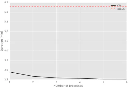
3.3.3.2.3 Scalability Comparison The implementation suggested in this

work contains process-level parallelization of computation MF component 25

1 2 3 4 5 6 Number of processes 2.5 3.0 3.5 4.0 4.5 5.0 5.5 6.0 6.5 Duration [min] CDL osCDL

Figure 3.4: Scalability: original simplified CDL (loosely dashed) and proposed CDL (solid) implemenation

compared to the proposed implementation of the author of CDL. The Fig-ure 3.4 shows comparison of these two implementations. For the compari-son, dataset CiteULike has been used, and models have beet set to the same hyper-parameters. The x-axis shows number of processes and the y-axis shows duration.

3.3.4 Algorithm Performance Evaluation

Due to the significant number of models that have to be evaluated during hyper-parameter optimization, it is necessary to have a fast evaluation. Be-cause the chosen measures allow to evaluate each user separately, similarly to 3.3.3.1.1, process-level parallelization has been used for reduction of evaluation time.

3.3.5 Fine-tuning pipeline

Ready-to-use optimizers from the package scikit-optimizer have been used in a fine-tuning pipeline. Based on the analysis in section 1.3, a Bayesian optimization using Gaussian Processes (function gp minimize) and a random search by uniform sampling (function dummy minimize) have been selected.

The entire fine-tuning environment has been implemented in Jupyter Note-book. The code in Jupyter Notebooks is separated into cells, each cell can be run repeatedly and in any order, while variables are shared among cells, moreover it enable to render charts directly in the IDE, all these features make

3.3. Implementation

Jupyter Notebook an ideal tool for comfortable hyper-parameters tuning, re-sponding to results and reporting them.

The whole fine-tuning procedure can be described by following steps:

• loading data from disk,

• setting searching space of hyper-parameters,

• running optimizer,

• storing results to disk,

• loading results,

Chapter

4

Experiments

Experiments are conducted on one public dataset and two nonpublic datasets from different domains. The goal of the experiments is to compare two hyper-optimization technique and also compare two algorithms quantitatively.

4.1

Datasets

Within the scope of this work, three datasets from a different real-world do-mains for experiments were chosen. The first CiteULike has been used in [27] for evaluation CDL performance and it is available from 26. CiteULike allows users to create their own collections of articles. There are abstract, title, and tags for each article. It contains 5551 users, 16980 items and 49960 interac-tions. The remaining three datasets are not public and have been provided by the company Recombee 27.

One of nonpublic datasets, henceforth Fashion, contains data about user-item interactions as detail views, purchases, bookmarks and user-items description as a price, categories, a brand, a title, a link to an image. Fashion dataset contains ca. 100 000 items, 8 million users, 30 millions of items detail views and about 2 million purchases.

The last dataset comes from news webpage, henceforth News. Besides user-item interactions it contains article features such as a title, tags, and authors of articles. It contains about 450 000 articles, 100 million users and 600 million interactions.

4.2

Evaluation Scheme

Due to the size of nonpublic datasets and vast amount of experiments during fine-tuning, each dataset has been subsampled to approximately 25 000 users.

26

http://www.wanghao.in/CDL.htm 27

Further, users in each dataset have been randomly divided into two non-overlapping subsets (90 % training, 10 % testing), see 2.2.2. The training set consists of 90 % of users with all their interactions. The testing set consist of the remaining 10 % users. Items that are not in the training set are removed from the testing set. For each user in the testing set, we hide an item in his history, the remaining items are used to calculate user’s latent representation. The latent representation is used to calculate personalized recommendations. We repeat this procedure N times. Furthermore we record list of top K

recommended items and if the hidden item appears in it. The number of successful trials divided by min(K , #user0s interactions−1) (see 2.5) is value of user’s recall. N recorded lists are used to calculate coverage according to 2.6. K and N have been set to 10 during evaluation.

4.3

Experimental Settings

At first, the original simplified CDL implementation (osCDL) has been eval-uated and compared to CDL implementation proposed in this thesis (nCDL). For this purpose, the dataset CiteUlike has been used. Other evaluations have been done on datasets CiteULike, Fashion and News with proposed im-plementation 2.1.2. The Fashion dataset has been evaluated in two variants of auxiliary information. First, the text features have been leveraged and later image embeddings. The optimization algorithms have been set to the default settigns except number of calls and for GP the acquisition function has been set toEIs. In this setting, GP takes into account the function compute time and expected improvement. According to 2.2.2, suitable hyper-parameters for fine-tuning have been identified for MF and CDL. This has been done based on first optimization procedure by random search algorithm. The MF suitable hyper-parameters are:

• size of latent representation,

• regularization,

• weight of observed ratings,

• activation of user and item bias term,

• score computation method.

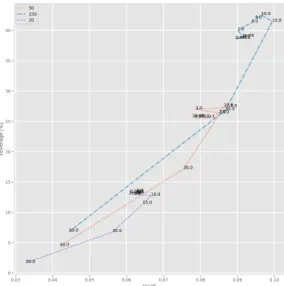
An ideal number of iterations has oscillated around number 15. Because the time complexity grows cubicly with the size of latent representation, the size has been fixed to 80 for further experiments. The Figure 4.3 shows relation between size of latent representation and recall-coverage curves.

The CDL hyper-parameters suitable for fine-tuning are: