Gaussian Process Planning with Lipschitz Continuous Reward Functions

Gaussian Process Planning with Lipschitz Continuous Reward Functions:

Towards Unifying Bayesian Optimization, Active Learning, and Beyond

Chun Kai Ling

∗

and

Kian Hsiang Low

∗

and

Patrick Jaillet

† Department of Computer Science, National University of Singapore, Republic of Singapore∗ Department of Electrical Engineering and Computer Science, Massachusetts Institute of Technology, USA†

{chunkai, lowkh}@comp.nus.edu.sg∗, [email protected]†

Abstract

This paper presents a novel nonmyopic adaptive Gaus-sian process planning(GPP) framework endowed with a general class of Lipschitz continuous reward func-tions that can unify some active learning/sensing and Bayesian optimization criteria and offer practition-ers some flexibility to specify their desired choices for defining new tasks/problems. In particular, it uti-lizes a principled Bayesian sequential decision prob-lem framework for jointly and naturally optimizing the exploration-exploitation trade-off. In general, the re-sulting induced GPP policy cannot be derived exactly due to an uncountable set of candidate observations. A key contribution of our work here thus lies in ex-ploiting the Lipschitz continuity of the reward func-tions to solve for a nonmyopic adaptive-optimal GPP

(-GPP) policy. To plan in real time, we further pro-pose an asymptotically optimal, branch-and-bound any-time variant of-GPP with performance guarantee. We empirically demonstrate the effectiveness of our-GPP policy and its anytime variant in Bayesian optimization and an energy harvesting task.

1

Introduction

The fundamental challenge of integrated planning and learn-ing is to design an autonomous agent that can plan its ac-tions to maximize its expected total rewards while interact-ing with an unknown task environment. Recent research ef-forts tackling this challenge have progressed from the use of simple Markov models assuming discrete-valued, inde-pendent observations (e.g., inBayesian reinforcement learn-ing (BRL) (Poupart et al. 2006)) to that of a rich class of Bayesian nonparametricGaussian process(GP) models characterizing continuous-valued, correlated observations in order to represent the latent structure of more complex, pos-sibly noisy task environments with higher fidelity. Such a challenge is posed by the following important problems in machine learning, among others:

Active learning/sensing (AL). In the context of environ-mental sensing (e.g., adaptive sampling in oceanography (Leonard et al. 2007), traffic sensing (Chen et al. 2012; Chen, Low, and Tan 2013; Chen et al. 2015)), its objec-tive is to select the most informaobjec-tive (possibly noisy) ob-servations for predicting a spatially varying environmental Copyright c2016, Association for the Advancement of Artificial Intelligence (www.aaai.org). All rights reserved.

field (i.e., task environment) modeled by a GP subject to some sampling budget constraints (e.g., number of sensors, energy consumption). The rewards of an AL agent are de-fined based on some formal measure of predictive uncer-tainty such as the entropy or mutual information criterion. To resolve the issue of sub-optimality (i.e., local maxima) faced by greedy algorithms (Krause, Singh, and Guestrin 2008; Low et al. 2012; Ouyang et al. 2014; Zhang et al. 2016), re-cent developments have made nonmyopic AL computation-ally tractable with provable performance guarantees (Cao, Low, and Dolan 2013; Hoang et al. 2014; Low, Dolan, and Khosla 2009; 2008; 2011), some of which have fur-ther investigated the performance advantage of adaptivity by proposing nonmyopic adaptive observation selection poli-cies that depend on past observations.

Bayesian optimization (BO).Its objective is to select and gather the most informative (possibly noisy) observations for finding the global maximum of an unknown, highly complex (e.g., non-convex, no closed-form expression nor derivative) objective function (i.e., task environment) mod-eled by a GP given a sampling budget (e.g., number of costly function evaluations). The rewards of a BO agent are defined using an improvement-based (Brochu, Cora, and de Freitas 2010) (e.g.,probability of improvement(PI) orexpected im-provement (EI) over currently found maximum), entropy-based (Hennig and Schuler 2012; Hern´andez-Lobato, Hoff-man, and Ghahramani 2014), or upper confidence bound

(UCB) acquisition function (Srinivas et al. 2010). A limi-tation of most BO algorithms is that they are myopic. To overcome this limitation, approximation algorithms for non-myopic adaptive BO (Marchant, Ramos, and Sanner 2014; Osborne, Garnett, and Roberts 2009) have been proposed, but their performances are not theoretically guaranteed.

General tasks/problems.In practice, other types of rewards (e.g., logarithmic, unit step functions) need to be specified for an agent to plan and operate effectively in a given real-world task environment (e.g., natural phenomenon like wind or temperature) modeled by a GP, as detailed in Section 2.

As shall be elucidated later, similarities in the structure of the above problems motivate us to consider whether it is possible to tackle the overall challenge by devising a nonmy-opic adaptive GP planning framework with a general class of reward functions unifying some AL and BO criteria and affording practitioners some flexibility to specify their

de-sired choices for defining new tasks/problems. Such an in-tegrated planning and learning framework has to address the exploration-exploitation trade-off common to the above problems: The agent faces a dilemma between gathering ob-servations to maximize its expected total rewards given its current, possibly imprecise belief of the task environment (exploitation) vs. that to improve its belief to learn more about the environment (exploration).

This paper presents a novel nonmyopic adaptiveGaussian process planning (GPP) framework endowed with a gen-eral class of Lipschitz continuous reward functions that can unify some AL and BO criteria (e.g., UCB) discussed earlier and offer practitioners some flexibility to specify their de-sired choices for defining new tasks/problems (Section 2). In particular, it utilizes a principled Bayesian sequential deci-sion problem framework for jointly and naturally optimizing the exploration-exploitation trade-off, consequently allow-ing plannallow-ing and learnallow-ing to be integrated seamlessly and performed simultaneously instead of separately (Deisenroth, Fox, and Rasmussen 2015). In general, the resulting induced GPP policy cannot be derived exactly due to an uncount-able set of candidate observations. A key contribution of our work here thus lies in exploiting the Lipschitz continu-ity of the reward functions to solve for a nonmyopic adap-tive-optimal GPP(-GPP) policy given an arbitrarily user-specified loss bound (Section 3). To plan in real time, we further propose an asymptotically optimal, branch-and-bound anytime variant of-GPP with performance guaran-tee. Finally, we empirically evaluate the performances of our

-GPP policy and its anytime variant in BO and an energy harvesting task on simulated and real-world environmental fields (Section 4). To ease exposition, the rest of this paper will be described by assuming the task environment to be an environmental field and the agent to be a mobile robot, which coincide with the setup of our experiments.

2

Gaussian Process Planning (GPP)

Notations and Preliminaries. LetS be the domain of an environmental field corresponding to a set of sampling lo-cations. At time step t > 0, a robot can deterministically move from its previous locationst−1to visit locationst ∈

A(st−1)and observes it by taking a corresponding realized

(random) field measurement zt(Zt) where A(st−1) ⊆ S

denotes a finite set of sampling locations reachable from its previous locationst−1in a single time step. The state of the

robot at its initial starting locations0is represented by prior

observations/data d0 , hs0,z0i available before planning

wheres0andz0denote, respectively, vectors comprising

lo-cations visited/observed and corresponding field measure-ments taken by the robot prior to planning ands0is the last

component ofs0. Similarly, at time stept >0, the state of

the robot at its current locationstis represented by obser-vations/datadt ,hst,ztiwherest ,s0⊕(s1,· · ·st)and

zt,z0⊕(z1,· · ·zt)denote, respectively, vectors compris-ing locations visited/observed and correspondcompris-ing field mea-surements taken by the robot up until time step tand ‘⊕’ denotes vector concatenation. At time stept >0, the robot also receives a rewardR(zt,st)to be defined later.

Modeling Environmental Fields with Gaussian Processes

(GPs).The GP can be used to model a spatially varying en-vironmental field as follows: The field is assumed to be a re-alization of a GP. Each locations∈ Sis associated with a la-tent field measurementYs. LetYS ,{Ys}s∈Sdenote a GP, that is, every finite subset ofYS has a multivariate Gaussian distribution (Rasmussen and Williams 2006). Then, the GP is fully specified by itspriormeanµs ,E[Ys]and covari-ancekss0 ,cov[Y_s, Y_s0]for alls, s0 ∈ S, the latter of which characterizes the spatial correlation structure of the environ-ment field and can be defined using a covariance function. A common choice is the squared exponential covariance func-tionkss0 ,σ2_yexp{−0.5(s−s0)>M−2(s−s0)}whereσ2_yis the signal variance controlling the intensity of measurements andM is a diagonal matrix with length-scale componentsl1

andl2 governing the degree of spatial correlation or

“sim-ilarity” between measurements in the respective horizontal and vertical directions of the2D fields in our experiments.

The field measurements taken by the robot are assumed to be corrupted by Gaussian white noise, i.e.,Zt,Yst+ε

whereε∼ N(0, σ2

n)andσ2nis the noise variance. Suppos-ing the robot has gathered observationsdt = hst,ztifrom time steps0tot, the GP model can perform probabilistic re-gression by usingdtto predict the noisy measurement at any unobserved locationst+1∈ A(st)as well as provide its pre-dictive uncertainty using a Gaussian prepre-dictive distribution

p(zt+1|dt, st+1) =N(µst+1|dt, σ 2

st+1|st)with the following

posteriormean and variance, respectively:

µst+1|dt,µst+1+ Σst+1stΓ −1 stst(zt−µst) > σ2_s t+1|st,kst+1st+1+σ 2 n−Σst+1stΓ −1 ststΣstst+1

whereµstis a row vector with mean componentsµsfor

ev-ery locationsofst,Σst+1stis a row vector with covariance

componentskst+1sfor every locationsofst,Σstst+1 is the

transpose of Σst+1st, andΓstst , Σstst +σ 2

nI such that

Σststis a covariance matrix with componentskss0for every

pair of locationss, s0ofst. An important property of the GP model is that, unlikeµst+1|dt,σ

2

st+1|stis independent ofzt. Problem Formulation. To frame nonmyopic adaptive

Gaussian process planning(GPP) as a Bayesian sequential decision problem, let an adaptive policyπbe defined to se-quentially decide the next locationπ(dt)∈ A(st)to be ob-served at each time steptusing observationsdtover a finite planning horizon ofHtime steps/stages (i.e., sampling bud-get of H locations). The value Vπ

0 (d0)under an adaptive

policyπis defined to be the expected total rewards achieved by its selected observations when starting with some prior observationsd0and followingπthereafter and can be

com-puted using the followingH-stage Bellman equations:

Vπ t (dt),Qtπ(dt, π(dt)) Qπ t(dt, st+1),E[R(Zt+1,st+1) + Vπ t+1(hst+1,zt⊕Zt+1i)|dt, st+1]

for stages t = 0, . . . , H −1 where Vπ

H(dH) , 0. To solve the GPP problem, the notion of Bayes-optimalityis exploited for selecting observations to achieve the largest possible expected total rewards with respect to all possi-ble induced sequences of future Gaussian posterior beliefs

Formally, this involves choosing an adaptive policy π to maximizeVπ

0 (d0), which we call the GPP policyπ∗. That

is,V₀∗(d0) , Vπ ∗ 0 (d0) = maxπV0π(d0). By pluggingπ∗ intoVπ t (dt)andQtπ(dt, st+1)above, Vt∗(dt),maxst+1∈A(st)Q ∗ t(dt, st+1) Q∗_t(dt, st+1),E[R(Zt+1,st+1)|dt, st+1] + E[Vt∗+1(hst+1,zt⊕Zt+1i)|dt, st+1] (1)

for stages t = 0, . . . , H −1 where V_H∗(dH) , 0. To see how the GPP policy π∗ _{jointly and naturally} opti-mizes the exploration-exploitation trade-off, its selected lo-cation π∗(dt) = arg maxst+1∈A(st)Q

∗

t(dt, st+1) at each

time step t affects both the immediate expected reward E[R(Zt+1,st ⊕ π∗(dt))|dt, π∗(dt)] given current belief

p(zt+1|dt, π∗(dt))(i.e., exploitation) as well as the Gaussian posterior beliefp(zt+2|hst⊕π∗(dt),zt⊕zt+1i, π∗(hst⊕

π∗_(d

t),zt⊕zt+1i)) at next time step t + 1 (i.e., explo-ration), the latter of which influences expected future re-wardsE[Vt∗+1(hst⊕π∗(dt),zt⊕Zt+1i)|dt, π∗(dt)].

In general, the GPP policyπ∗cannot be derived exactly because the expectation terms in (1) usually cannot be eval-uated in closed form due to an uncountable set of candidate measurements (Section 1) except for degenerate cases like

R(zt+1,st+1) being independent ofzt+1 andH ≤ 2. To

overcome this difficulty, we will show in Section 3 later how the Lipschitz continuity of the reward functions can be ex-ploited for theoretically guaranteeing the performance of our proposed nonmyopic adaptive-optimal GPP policy, that is, the expected total rewards achieved by its selected observa-tions closely approximates that of π∗ within an arbitrarily user-specified loss bound >0.

Lipschitz Continuous Reward Functions. R(zt,st) ,

R1(zt)+R2(zt)+R3(st)whereR1,R2, andR3are

user-de-fined reward functions that satisfy the conditions below:

• R1(zt)is Lipschitz continuous inztwith Lipschitz con-stant `1. So,hσ(u) , (R1∗ N(0, σ2))(u) is Lipschitz

continuous inuwith`1where ‘∗’ denotes convolution; • R2(zt): Definegσ(u) , (R2 ∗ N(0, σ2))(u)such that

(a)gσ(u)is well-defined for allu∈R, (b)gσ(u)can be evaluated in closed form or computed up to an arbitrary precision in reasonable time for allu∈R, and (c)gσ(u)is Lipschitz continuous1_{inuwith Lipschitz constant`}

2(σ); • R3(st)only depends on locationsstvisited/observed by the robot up until time steptand is independent of real-ized measurement zt. It can be used to represent some sampling or motion costs or explicitly consider explo-ration by defining it as a function ofσ2

st+1|st.

Using the above definition ofR(zt,st), the immediate ex-pected reward in (1) evaluates toE[R(Zt+1,st+1)|dt, st+1] = (hσ_st

+1|st+gσst+1|st)µst+1|dt

+R3(st+1)which is

Lip-schitz continuous in the realized measurementszt:

Lemma 1 Letα(st+1),kΣst+1stΓ −1 ststkandd 0 t,hst,z0ti. Then,|E[R(Zt+1,st+1)|dt,st+1]−E[R(Zt+1,st+1)|d0t,st+1]| ≤α(st+1) `1+`2(σst+1|st) kzt−z0tk. 1

UnlikeR1,R2 does not need to be Lipschitz continuous (or

continuous); it must only be Lipschitz continuous after convolution with any Gaussian kernel. An example ofR2is unit step function.

Its proof is in (Ling, Low, and Jaillet 2016). Lemma 1 will be used to prove the Lipschitz continuity ofV_t∗in (1) later. Before doing this, let us consider how the Lipschitz continu-ous reward functions defined above can unify some AL and BO criteria discussed in Section 1 and be used for defining new tasks/problems.

Active learning/sensing (AL). Setting R(zt+1,st+1) =

R3(st+1) = 0.5 log(2πeσ_s2_t+1|st) yields the well-known

nonmyopic AL algorithm calledmaximum entropy sampling

(MES) (Shewry and Wynn 1987) which plans/decides loca-tions with maximum entropy to be observed that minimize the posterior entropy remaining in the unobserved areas of the field. Since R(zt+1,st+1) is independent of zt+1, the

expectations in (1) go away, thus making MES non-adaptive and hence a straightforward search algorithm not plagued by the issue of uncountable set of candidate measurements. As such, we will not focus on such a degenerate case. This degeneracy vanishes when the environment field is instead a realization of log-Gaussian process. Then, MES becomes adaptive (Low, Dolan, and Khosla 2009) and its reward function can be represented by our Lipschitz continuous re-ward functions: By settingR1(zt+1) = 0,R2andgσ_st

+1|st

as identity functions with`2(σst+1|st) = 1, andR3(st+1) = 0.5 log(2πeσ2

st+1|st), E[R(Zt+1,st+1)|dt, st+1] =

µst+1|dt+ 0.5 log(2πeσ 2

st+1|st).

Bayesian optimization (BO). The greedy BO algorithm of Srinivas et al. (2010) utilizes the UCB selection crite-rion µst+1|dt +βσst+1|st (β ≥ 0) to approximately

opti-mize the global BO objective of total field measurements

PH

t=1zttaken by the robot or, equivalently, minimize its to-tal regret. UCB can be represented by our Lipschitz con-tinuous reward functions: By setting R1(zt+1) = 0, R2

and gσ_st

+1|st as identity functions with`2(σst+1|st) = 1,

and R3(st+1) = βσst+1|st, E[R(Zt+1,st+1)|dt, st+1] =

µst+1|dt +βσst+1|st. In particular, when β = 0, it can be

derived that our GPP policyπ∗_{maximizes theexpected} to-tal field measurements taken by the robot, hence optimizing the exact global BO objective of Srinivas et al. (2010) in the expected sense. So, unlike greedy UCB, our nonmyopic GPP framework does not have to explicitly consider an ad-ditional weighted exploration term (i.e.,βσst+1|st) in its

re-ward function because it can jointly and naturally optimize the exploration-exploitation trade-off, as explained earlier. Nevertheless, if a stronger exploration behavior is desired (e.g., in online planning), thenβ has to be fine-tuned. Dif-ferent from nonmyopic BO algorithm of Marchant, Ramos, and Sanner (2014) using UCB-based rewards, our proposed nonmyopic-optimal GPP policy (Section 3) does not need to impose an extreme assumption of maximum likelihood observations during planning and, more importantly, pro-vides a performance guarantee, including for the extreme assumption made by nonmyopic UCB. Our GPP framework differs from nonmyopic BO algorithm of Osborne, Garnett, and Roberts (2009) in that every selected observation con-tributes to the total field measurements taken by the robot instead of considering just the expected improvement for the last observation. So, it usually does not have to expend all

the given sampling budget to find the global maximum.

General tasks/problems.In practice, the necessary reward function can be more complex than the ones specified above that are formed from an identity function of the field mea-surement. For example, consider the problem of placing wind turbines in optimal locations to maximize the total power production. Though the average wind speed in a re-gion can be modeled by a GP, the power output is not a linear function of the steady-state wind speed. In fact, power pro-duction requires a certain minimum speed known as the cut-in speed. After this threshold is met, power output cut-increases and eventually plateaus. Assuming the cut-in speed is1, this effect can be modeled with a logarithmic reward function2_: R(zt+1,st+1) = R1(zt+1) gives a value of log(zt+1) if

zt+1 > 1, and0 otherwise where `1 = 1. To the best of

our knowledge,hσ_st+1|s_t(u)has no closed-form expression. In (Ling, Low, and Jaillet 2016), we present other interesting reward functions like unit step function1 and Gaussian dis-tribution that can be represented byR(zt+1,st+1)and used

in real-world tasks.

Theorem 1 below reveals thatVt∗(dt)(1) with Lipschitz continuous reward functions is Lipschitz continuous in zt with Lipschitz constantLt(st)defined below:

Definition 1 LetLH(sH), 0. Fort = 0, . . . , H−1,

de-fineLt(st),maxst+1∈A(st)α(st+1) `1+`2(σst+1|st)

+

Lt+1(st+1) p

1 +α(st+1)2.

Theorem 1 (Lipschitz Continuity ofV_t∗) For

t= 0, . . . , H,|V∗

t(dt)−Vt∗(d0t)| ≤Lt(st)kzt−z0tk. Its proof uses Lemma 1 and is in (Ling, Low, and Jaillet 2016). The result below is a direct consequence of Theo-rem 1 and will be used to theoretically guarantee the perfor-mance of our proposed nonmyopic adaptive-optimal GPP policy in Section 3:

Corollary 1 For t = 0, . . . , H, |Vt∗(hst,zt−1 ⊕zti) −

V_t∗(hst,zt−1⊕z0ti)| ≤Lt(st)|zt−zt0|.

3

-Optimal GPP (

-GPP)

The key idea of constructing our proposed nonmyopic adap-tive-GPP policy is to approximate the expectation terms in (1) at every stage using a form of deterministic sampling, as illustrated in the figure below. Specifically, the measure-ment space ofp(zt+1|dt, st+1)is first partitioned inton≥2

intervals ζ0, . . . , ζn−1 such that intervals ζ1, . . . , ζn−2 are

equally spaced within the bounded gray region[µst+1|dt −

τ σst+1|st, µst+1|dt +τ σst+1|st] specified by a user-defined

width parameterτ ≥0while intervalsζ0andζn−1span the

two infinitely long red tails. Note thatτ >0requiresn >2

for the partition to be valid. The n sample measurements

z0. . . zn−1 are then selected by setting z0 as upper limit of red intervalζ0,zn−1as lower limit of red intervalζn−1,

andz1, . . . , zn−2as centers of the respective gray intervals

ζ1, . . . , ζn−2. Next, the weights w0. . . wn−1 for the

cor-responding sample measurementsz0, . . . , zn−1are defined as the areas under their respective intervals ζ0, . . . , ζn−1

of the Gaussian predictive distributionp(zt+1|dt, st+1). So, 2

In reality, the speed-power relationship is not exactly logarith-mic, but this approximation suffices for the purpose of modeling.

p(zt+1|dt, st+1) z0_,µ st+1|dt−τ σst+1|st; zn−1_,µ st+1|dt+τ σst+1|st; zi ,z0₊i−0.5 n−2(z n−1_−z0₎ fori= 1, . . . , n−2. wi ,Φ(2iτ n−2−τ)−Φ( 2(i−1)τ n−2 −τ) fori= 1, . . . , n−2; w0_=wn−1 ,Φ(−τ). z0 w0 z1 w1 . . . . . . . . . . . . zi-1 wi-1 zi wi zi+1 wi+1 zn-1 wn-1 zn-2 wn-2 . . . . . . . . . . . . zt+1 ζ1 ζi-1 ζi ζi+1 ζn-2 ζ0 ζn-1 Pn−1 i=0 w

i _{= 1. An example of such a partition is given in} (Ling, Low, and Jaillet 2016). The selected sample measure-ments and their corresponding weights can be exploited for approximating Vt∗ with Lipschitz continuous reward func-tions (1) using the followingH-stage Bellman equations:

V t(dt),maxst+1∈A(st)Q t(dt, st+1) Q t(dt, st+1),gσ_st +1|st µst+1|dt +R3(st+1) + n−1 X i=0 wi R1(zi) +Vt+1(hst+1,zt⊕zii) (2)

for stagest= 0, . . . , H−1whereV

H(dH),0. The result-ing induced-GPP policyπjointly and naturally optimizes the exploration-exploitation trade-off in a similar manner as that of the GPP policyπ∗, as explained in Section 2. It is interesting to note that setting τ = 0yieldsz0 _{= . . . =}

zn−1 _{= µ}

st+1|dt, which is equivalent to selecting a single

sample measurement ofµst+1|dt with corresponding weight

of1. This is identical to the special case of maximum likeli-hood observations during planning which is the extreme as-sumption used by nonmyopic UCB (Marchant, Ramos, and Sanner 2014) for sampling to gain time efficiency.

Performance Guarantee. The difficulty in theoretically guaranteeing the performance of our-GPP policyπ(i.e., relative to that of GPP policyπ∗) lies in analyzing how the values of the width parameterτand deterministic sampling sizencan be chosen to satisfy the user-specified loss bound

, as discussed below. The first step is to prove thatV t in (2) approximatesV_t∗ in (1) closely for some chosenτ and

nvalues, which relies on the Lipschitz continuity ofV_t∗in Corollary 1. DefineΛ(n, τ)to be equal to the value ofp2/π

ifn≥2∧τ = 0, and value ofκ(τ)+η(n, τ)ifn >2∧τ >0

whereκ(τ)_,p2/πexp(−0.5τ2_{)−2τΦ(−τ),η(n, τ)} ,

2τ(0.5−Φ(−τ))/(n−2), andΦis a standard normal CDF.

Theorem 2 Suppose thatλ > 0 is given. For all dt and

t= 0, . . . , H, if

λ≥Λ(n, τ)σst+1|st(`1+Lt+1(st+1)) (3)

for allst+1∈ A(st), then|Vt(dt)−Vt∗(dt)| ≤λ(H−t). Its proof uses Corollary 1 and is given in (Ling, Low, and Jaillet 2016).

Remark 1. From Theorem 2, a tighter bound on the error

|V

t(dt)−Vt∗(dt)|can be achieved by decreasing the sam-pling budget ofHlocations3and increasing the determinis-tic sampling sizen; increasingnreducesη(n, τ)and hence

3

Λ(n, τ), which allowsλto be reduced as well. The width parameterτ has a mixed effect on this error bound: Note thatκ(τ)(η(n, τ)) is proportional to some upper bound on the error incurred by the extreme sample measurementsz0

andzn−1_(z1_{, . . . , z}n−2_{), as shown in (Ling, Low, and}

Jail-let 2016). Increasingτreducesκ(τ)but unfortunately raises

η(n, τ). So, in order to reduce Λ(n, τ)further by increas-ingτ, it has to be complemented by raisingnfast enough to keepη(n, τ)from increasing. This allowsλto be reduced further as well.

Remark 2. A feasible choice ofτ andnsatisfying (3) can be expressed analytically in terms of the givenλand hence computed prior to planning, as shown in (Ling, Low, and Jaillet 2016).

Remark 3. σst+1|st and Lt+1(st+1) for all st+1 and t = 0, . . . , H−1can be computed prior to planning as they de-pend ons0 and all reachable locations from s0 but not on

their measurements.

Using Theorem 2, the next step is to bound the perfor-mance loss of our-GPP policyπ _{relative to that of GPP} policyπ∗_{, that is, policyπis-optimal:}

Theorem 3 Given the user-specified loss bound > 0,

V₀∗(d0)−Vπ

0 (d0)≤by substitutingλ=/(H(H + 1))

into the choice ofτandnstated in Remark2above.

Its proof is in (Ling, Low, and Jaillet 2016). It can be ob-served from Theorem 3 that a tighter boundon the error

V₀∗(d0)−Vπ

0 (d0)can be achieved by decreasing the

sam-pling budget ofH locations3 _{and increasing the}

determin-istic sampling size n. The effect of width parameterτ on this error boundis the same as that on the error bound of

|Vt(dt)−Vt∗(dt)|, as explained in Remark1above.

Anytime-GPP.Unlike GPP policyπ∗, our-GPP policy

π_{can be derived exactly since its incurred time is} indepen-dent of the size of the uncountable set of candidate mea-surements. However, expanding the entire search tree of -GPP (2) incurs time containing aO(nH_{)term and is not} always necessary to achieve-optimality in practice. To mit-igate this computational difficulty4_{, we propose an anytime}

variant of -GPP that can produce a good policy fast and improve its approximation quality over time, as briefly dis-cussed here and detailed with the pseudocode in (Ling, Low, and Jaillet 2016).

The key intuition is to expand the sub-trees rooted at “promising” nodes with the highest weighted uncertainty of their corresponding valuesVt∗(dt)so as to improve their es-timates. To represent such uncertainty at each encountered node, upper & lower heuristic bounds (respectively,V∗_t(dt) andV∗t(dt)) are maintained, like in (Smith and Simmons 2006). A partial construction of the entire tree is maintained and expanded incrementally in each iteration of anytime -GPP that incurs linear time innand comprises3steps:

Node selection.Traverse down the partially constructed tree by repeatedly selecting nodes with largest difference be-tween their upper and lower bounds (i.e., uncertainty) dis-counted by weightwi∗of its preceding sample measurement

4

The value ofnis a bigger computational issue than that ofH

whenis small and in online planning.

zi∗until an unexpanded node, denoted bydt, is reached.

Expand tree.Construct a “minimal” sub-tree rooted at node

dtby sampling all possible next locations and only their me-dian sample measurementsz¯irecursively up to full heightH.

Backpropagation. Backpropagate bounds from the leaves of the newly constructed sub-tree to nodedt, during which the refined bounds of expanded nodes are used to inform the bounds of unexpanded siblings by exploiting the Lipschitz continuity ofV∗

t (Corollary 1), as explained in (Ling, Low, and Jaillet 2016). Backpropagate bounds to the root of the partially constructed tree in a similar manner.

By using the lower heuristic bound to produce our any-time-GPP policy, its performance loss relative to that of GPP policy π∗ can be bounded, as proven in (Ling, Low, and Jaillet 2016).

4

Experiments and Discussion

This section empirically evaluates the online planning per-formance and time efficiency of our-GPP policyπ_{and its} anytime variant under limited sampling budget in an energy harvesting task on a simulated wind speed field and in BO on simulated plankton density (chl-a) field and real-world log-potassium (lg-K) concentration (mg l−1_{) field (Ling, Low,}

and Jaillet 2016) of Broom’s Barn farm (Webster and Oliver 2007). Each simulated (real-world lg-K) field is spatially distributed over a0.95km by0.95km (520 m by440m) region discretized into a20×20(14×12) grid of sampling locations. These fields are assumed to be realizations of GPs. The wind speed (chl-a) field is simulated using hyperparam-etersµs= 0,5l1=l2= 0.2236(0.2) km,σ2n= 10−5, and

σ2y = 1. The hyperparameters µs = 3.26,l1 = 42.8 m,

l2 = 103.6 m, σ2n = 0.0222, and σ2y = 0.057 of lg-K field are learned using maximum likelihood estimation (Ras-mussen and Williams 2006). The robot’s initial starting lo-cation is near to the center of each simulated field and ran-domly selected for lg-K field. It can move to any of its 4

adjacent grid locations at each time step and is tasked to maximize its total rewards over20time steps (i.e., sampling budget of20locations).

In BO, the performances of our-GPP policyπ _{and its} anytime variant are compared with that of state-of-the-art

nonmyopic UCB(Marchant, Ramos, and Sanner 2014) and

greedy PI, EI, UCB (Brochu, Cora, and de Freitas 2010; Srinivas et al. 2010). Three performance metrics are used: (a) Total rewards achieved over the evolved time steps (i.e., higher total rewards imply less total regret in BO (Sec-tion 2)), (b) maximum reward achieved during experiment, and (c) search tree size in terms of no. of nodes (i.e., larger tree size implies higher incurred time). All experiments are run on a Linux machine with Intel Core i5at1.7GHz.

Energy Harvesting Task on Simulated Wind Speed Field.

A robotic rover equipped with a wind turbine is tasked to harvest energy/power from the wind while exploring a polar region (Chen et al. 2014). It is driven by the logarithmic re-ward function described under ‘General tasks/problems’ in Section 2. Fig. 1 shows results of performances of our-GPP

5

Its actual prior mean is not zero; we have applied zero-mean GP toYs−µsfor simplicity.

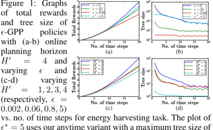
Figure 1: Graphs of total rewards and tree size of

-GPP policies with (a-b) online planning horizon H0 _{= 4 and} varying and (c-d) varying H0 = 1,2,3,4 (respectively, = 0.002,0.06,0.8,5) (a) (b) (c) (d)

vs. no. of time steps for energy harvesting task. The plot of

∗= 5uses our anytime variant with a maximum tree size of

5×104nodes while the plot of= 250effectively assumes maximum likelihood observations during planning like that of nonmyopic UCB (Marchant, Ramos, and Sanner 2014). policy and its anytime variant averaged over 30 indepen-dent realizations of the wind speed field. It can be observed that the gradients of the achieved total rewards (i.e., power production) increase over time, which indicate a higher ob-tained reward with an increasing number of time steps as the robot can exploit the environment more effectively with the aid of exploration from previous time steps. The gradients eventually stop increasing when the robot enters a perceived high-reward region. Further exploration is deemed unnec-essary as it is unlikely to find another preferable location withinH0time steps; so, the robot remains near-stationary for the remaining time steps. It can also be observed that the incurred time is much higher in the first few time steps. This is expected because the posterior varianceσst+1|stdecreases

with increasing time stept, thus requiring a decreasing de-terministic sampling sizento satisfy (3).

Initially, all-GPP policies achieve similar total rewards as the robots begin from the same starting location. After some time, -GPP policies with lower user-specified loss boundand longer online planning horizonH0_achieve con-siderably higher total rewards at the cost of more incurred time. In particular, it can be observed that a robot assum-ing maximum likelihood observations durassum-ing plannassum-ing (i.e.,

= 250) like that of nonmyopic UCB or using a greedy

policy (i.e.,H0 = 1) performs poorly very quickly. In the former case (Fig. 1a), the gradient of its total rewards stops increasing quite early (i.e., from time step9onwards), which indicates that its perceived local maximum is reached pre-maturely. Interestingly, it can be observed from Fig. 1d that the-GPP policy with H0 = 2and = 0.06incurs more time than that with H0 = 3and = 0.8 despite the lat-ter achieving higher total rewards. This suggests trading off tighter loss boundfor longer online planning horizonH0, especially when is too small that in turn requires a very largenand consequently incurs significantly more time4_.

BO on Real-World Log-Potassium Concentration Field.

An agricultural robot is tasked to find the peak lg-K mea-surement (i.e., possibly in an over-fertilized area) while ex-ploring the Broom’s Barn farm (Webster and Oliver 2007). It is driven by the UCB-based reward function described under ‘BO’ in Section 2. Fig. 2 shows results of performances of

(a) (b) (c)

Figure 2: Graphs of total normalized6rewards of-GPP poli-cies using UCB-based rewards with (a) H0 = 4, β = 0, and varying , (b) varying H0 = 1,2,3,4 (respectively,

= 0.002,0.003,0.4,2) andβ = 0, and (c)H0 = 4,= 1, and varyingβvs. no. of time steps for BO on real-world lg-K field. The plot of∗ = 1uses our anytime variant with a maximum tree size of3×104_{nodes while the plot of= 25}

effectively assumes maximum likelihood observations dur-ing planndur-ing like that of nonmyopic UCB.

our-GPP policy and its anytime variant, nonmyopic UCB (i.e.,= 25), and greedy PI, EI, UCB (i.e.,H0 = 1) aver-aged over 25randomly selected robot’s initial starting lo-cation. It can be observed from Figs. 2a and 2b that the gradients of the achieved total normalized6 rewards gener-ally increase over time. In particular, from Fig. 2a, nonmy-opic UCB assuming maximum likelihood observations dur-ing planndur-ing obtains much less total rewards than the other -GPP policies and the anytime variant after20time steps and finds a maximum lg-K measurement of3.62that is at least

0.4σyworse after20time steps. The performance of the any-time variant is comparable to that of our best-performing -GPP policy with= 3. From Fig. 2b, the greedy policy (i.e.,

H0 = 1) withβ = 0performs much more poorly than its nonmyopic-GPP counterparts and finds a maximum lg-K measurement of3.56that is lower than that of greedy PI and EI due to its lack of exploration. By increasingH0 to2-4, our-GPP policies withβ = 0outperform greedy PI and EI as they can naturally and jointly optimize the exploration-exploitation trade-off. Interestingly, Fig. 2c shows that our

-GPP policy withβ = 2achieves the highest total rewards after 20 time steps, which indicates the need of a slightly stronger exploration behavior than that with β = 0. This may be explained by a small length-scale (i.e., spatial corre-lation) of the lg-K field, thus requiring some exploration to find the peak measurement. By increasingH0 _{beyond4 or} with larger spatial correlation (Ling, Low, and Jaillet 2016), we expect a diminishing role of theβσst+1|st term. It can

also be observed that aggressive exploration (i.e.,β ≥ 10) hurts the performance. Results of the tree size (i.e., incurred time) of our -GPP policy and its anytime variant are in (Ling, Low, and Jaillet 2016).

5

Conclusion

This paper describes a novel nonmyopic adaptive -GPP framework endowed with a general class of Lipschitz con-tinuous reward functions that can unify some AL and BO criteria and be used for defining new tasks/problems. In par-ticular, it can jointly and naturally optimize the exploration-exploitation trade-off. We theoretically guarantee the perfor-mances of our-GPP policy and its anytime variant and em-pirically demonstrate their effectiveness in BO and an

en-6

To ease interpretation of the results, each reward is normalized by subtracting the prior mean from it.

ergy harvesting task. For our future work, we plan to scale up-GPP and its anytime variant for big data using paral-lelization (Chen et al. 2013; Low et al. 2015), online learn-ing (Xu et al. 2014), and stochastic variational inference (Hoang, Hoang, and Low 2015) and extend them to handle unknown hyperparameters (Hoang et al. 2014).

Acknowledgments.This work was supported by Singapore-MIT Alliance for Research and Technology Subaward Agreement No.52R-252-000-550-592.

References

Brochu, E.; Cora, V. M.; and de Freitas, N. 2010. A tuto-rial on Bayesian optimization of expensive cost functions, with application to active user modeling and hierarchical re-inforcement learning. arXiv:1012.2599.

Cao, N.; Low, K. H.; and Dolan, J. M. 2013. Multi-robot in-formative path planning for active sensing of environmental phenomena: A tale of two algorithms. InProc. AAMAS. Chen, J.; Low, K. H.; Tan, C. K.-Y.; Oran, A.; Jaillet, P.; Dolan, J. M.; and Sukhatme, G. S. 2012. Decentralized data fusion and active sensing with mobile sensors for modeling and predicting spatiotemporal traffic phenomena. InProc. UAI, 163–173.

Chen, J.; Cao, N.; Low, K. H.; Ouyang, R.; Tan, C. K.-Y.; and Jaillet, P. 2013. Parallel Gaussian process regression with low-rank covariance matrix approximations. InProc. UAI, 152–161.

Chen, J.; Liang, J.; Wang, T.; Zhang, T.; and Wu, Y. 2014. Design and power management of a wind-solar-powered po-lar rover. Journal of Ocean and Wind Energy1(2):65–73. Chen, J.; Low, K. H.; Jaillet, P.; and Yao, Y. 2015. Gaussian process decentralized data fusion and active sensing for spa-tiotemporal traffic modeling and prediction in mobility-on-demand systems.IEEE Trans. Autom. Sci. Eng.12:901–921. Chen, J.; Low, K. H.; and Tan, C. K.-Y. 2013. Gaussian process-based decentralized data fusion and active sensing for mobility-on-demand system. InProc. RSS.

Deisenroth, M. P.; Fox, D.; and Rasmussen, C. E. 2015. Gaussian processes for data-efficient learning in robotics and control.IEEE Transactions on Pattern Analysis and Ma-chine Intelligence37(2):408–423.

Hennig, P., and Schuler, C. J. 2012. Entropy search for information-efficient global optimization. JMLR13:1809– 1837.

Hern´andez-Lobato, J. M.; Hoffman, M. W.; and Ghahra-mani, Z. 2014. Predictive entropy search for efficient global optimization of black-box functions. InProc. NIPS. Hoang, T. N.; Low, K. H.; Jaillet, P.; and Kankanhalli, M. 2014. Nonmyopic-Bayes-optimal active learning of Gaus-sian processes. InProc. ICML, 739–747.

Hoang, T. N.; Hoang, Q. M.; and Low, K. H. 2015. A unifying framework of anytime sparse Gaussian process re-gression models with stochastic variational inference for big data. InProc. ICML, 569–578.

Krause, A.; Singh, A.; and Guestrin, C. 2008. Near-optimal sensor placements in Gaussian processes: Theory, efficient algorithms and empirical studies. JMLR9:235–284.

Leonard, N. E.; Palley, D. A.; Lekien, F.; Sepulchre, R.; Fratantoni, D. M.; and Davis, R. E. 2007. Collective motion, sensor networks, and ocean sampling.Proc. IEEE95:48–74. Ling, C. K.; Low, K. H.; and Jaillet, P. 2016. Gaussian process planning with Lipschitz continuous reward func-tions: Towards unifying Bayesian optimization, active learn-ing, and beyond. arXiv:1511.06890.

Low, K. H.; Chen, J.; Dolan, J. M.; Chien, S.; and Thomp-son, D. R. 2012. Decentralized active robotic exploration and mapping for probabilistic field classification in environ-mental sensing. InProc. AAMAS, 105–112.

Low, K. H.; Yu, J.; Chen, J.; and Jaillet, P. 2015. Parallel Gaussian process regression for big data: Low-rank repre-sentation meets Markov approximation. InProc. AAAI. Low, K. H.; Dolan, J. M.; and Khosla, P. 2008. Adaptive multi-robot wide-area exploration and mapping. In Proc. AAMAS, 23–30.

Low, K. H.; Dolan, J. M.; and Khosla, P. 2009. Information-theoretic approach to efficient adaptive path planning for mobile robotic environmental sensing. InProc. ICAPS. Low, K. H.; Dolan, J. M.; and Khosla, P. 2011. Active Markov information-theoretic path planning for robotic en-vironmental sensing. InProc. AAMAS, 753–760.

Marchant, R.; Ramos, F.; and Sanner, S. 2014. Sequential Bayesian optimisation for spatial-temporal monitoring. In

Proc. UAI.

Osborne, M. A.; Garnett, R.; and Roberts, S. J. 2009. Gaus-sian processes for global optimization. InProc. 3rd Interna-tional Conference on Learning and Intelligent Optimization. Ouyang, R.; Low, K. H.; Chen, J.; and Jaillet, P. 2014. Multi-robot active sensing of non-stationary Gaussian process-based environmental phenomena. InProc. AAMAS. Poupart, P.; Vlassis, N.; Hoey, J.; and Regan, K. 2006. An analytic solution to discrete Bayesian reinforcement learn-ing. InProc. ICML, 697–704.

Rasmussen, C. E., and Williams, C. K. I. 2006. Gaussian Processes for Machine Learning. MIT Press.

Shewry, M. C., and Wynn, H. P. 1987. Maximum entropy sampling.J. Applied Statistics14(2):165–170.

Smith, T., and Simmons, R. 2006. Focused real-time dy-namic programming for MDPs: Squeezing more out of a heuristic. InProc. AAAI, 1227–1232.

Srinivas, N.; Krause, A.; Kakade, S.; and Seeger, M. 2010. Gaussian process optimization in the bandit setting: No re-gret and experimental design. InProc. ICML, 1015–1022. Webster, R., and Oliver, M. 2007.Geostatistics for Environ-mental Scientists. NY: John Wiley & Sons, Inc., 2nd edition. Xu, N.; Low, K. H.; Chen, J.; Lim, K. K.; and Ozgul, E. B. 2014. GP-Localize: Persistent mobile robot localization us-ing online sparse Gaussian process observation model. In

Proc. AAAI, 2585–2592.

Zhang, Y.; Hoang, T. N.; Low, K. H.; and Kankanhalli, M. 2016. Near-optimal active learning of multi-output Gaussian processes. InProc. AAAI.