Fast learning optimized prediction methodology (FLOPRED) for protein secondary structure prediction

Publications

Biochemistry, Biophysics and Molecular Biology

9-2012

Fast learning optimized prediction methodology

(FLOPRED) for protein secondary structure

prediction

Saras Saraswathi

The Research Institute at Nationwide Children’s Hospital

Juan Luis Fernandez-Martinez

University of Oviedo

Andrzej Kolinski

Robert L. Jernigan

Iowa State University, [email protected]

Andrzej Kloczkowski

The Research Institute at Nationwide Children’s Hospital

Follow this and additional works at:

http://lib.dr.iastate.edu/bbmb_ag_pubs

Part of the

Bioinformatics Commons

,

Genetics and Genomics Commons

, and the

Molecular

Biology Commons

The complete bibliographic information for this item can be found at

http://lib.dr.iastate.edu/

bbmb_ag_pubs/144

. For information on how to cite this item, please visit

http://lib.dr.iastate.edu/

howtocite.html

.

This Article is brought to you for free and open access by the Biochemistry, Biophysics and Molecular Biology at Iowa State University Digital Repository. It has been accepted for inclusion in Biochemistry, Biophysics and Molecular Biology Publications by an authorized administrator of Iowa State University Digital Repository. For more information, please [email protected].

Fast learning optimized prediction methodology (FLOPRED) for protein

secondary structure prediction

Abstract

Computational methods are rapidly gaining importance in the field of structural biology, mostly due to the explosive progress in genome sequencing projects and the large disparity between the number of sequences and the number of structures. There has been an exponential growth in the number of available protein sequences and a slower growth in the number of structures. There is therefore an urgent need to develop computational methods to predict structures and identify their functions from the sequence. Developing methods that will satisfy these needs both efficiently and accurately is of paramount importance for advances in many biomedical fields, including drug development and discovery of biomarkers. A novel method called Fast Learning Optimized PREDiction Methodology (FLOPRED) is proposed for predicting protein

secondary structure, using knowledge-based potentials combined with structure information from the CATH database. A Neural Network-based Extreme Learning Machine (ELM) and advanced Particle Swarm

Optimization (PSO) are used with this data that yield better and faster convergence to produce more accurate results. Protein secondary structures are predicted efficiently, reliably, more efficiently and more accurately using FLOPRED. These techniques yield superior classification of secondary structure elements, with a training accuracy ranging between 83% and 87% over a wide range of hidden neurons and a cross-validated testing accuracy ranging between 81% and 84% and a Segment OVerlap (SOV) score of 78% that are obtained with different sets of proteins. These results are comparable to other recently published studies, but are obtained with greater efficiencies, in terms of time and cost.

Keywords

Protein secondary structure prediction, Machine Learning, Particle swarm optimization, neural networks, knowledge-based potentials

Disciplines

Biochemistry, Biophysics, and Structural Biology | Bioinformatics | Genetics and Genomics | Molecular Biology

Comments

This is a manuscript of an article published as Saraswathi, Saras, Juan Luis Fernández-Martínez, Andrzej Koliński, Robert L. Jernigan, and Andrzej Kloczkowski. "Fast learning optimized prediction methodology (FLOPRED) for protein secondary structure prediction." Journal of molecular modeling 18, no. 9 (2012): 4275-4289.The final publication is available at Springer viahttp://dx.doi.org/10.1007/s00894-012-1410-7. Posted with permission.

Fast learning optimized prediction methodology (FLOPRED) for

protein secondary structure prediction

Saras Saraswathi,

Battelle Center for Mathematical Medicine, The Research Institute at Nationwide Children’s Hospital, 700 Children’s Drive, Columbus, OH, USA

Juan Luis Fernández-Martínez,

Department of Mathematics, University of Oviedo, Oviedo, Spain

Andrzej Kolinski,

Department of Mathematics, Laboratory of Theory of Biopolymers, Faculty of Chemistry, Warsaw University, Pasteura 1, 02-093 Warsaw

Robert L. Jernigan, and

Department of Biochemistry, Biophysics and Molecular Biology, Iowa State University, Ames, IA, USA

Andrzej Kloczkowski

Battelle Center for Mathematical Medicine, The Research Institute at Nationwide Children’s Hospital, 700 Children’s Drive, Columbus, OH, USA, Tel.: +1-614-722-3880 Fax:

+1-614-355-2728

Andrzej Kloczkowski: [email protected]

Abstract

Computational methods are rapidly gaining importance in the field of structural biology, mostly due to the explosive progress in genome sequencing projects and the large disparity between the number of sequences and the number of structures. There has been an exponential growth in the number of available protein sequences and a slower growth in the number of structures. There is therefore an urgent need to develop computational methods to predict structures and identify their functions from the sequence. Developing methods that will satisfy these needs both efficiently and accurately is of paramount importance for advances in many biomedical fields, including drug development and discovery of biomarkers. A novel method called Fast Learning Optimized PREDiction Methodology (FLOPRED) is proposed for predicting protein secondary structure, using knowledge-based potentials combined with structure information from the CATH database. A Neural Network-based Extreme Learning Machine (ELM) and advanced Particle Swarm Optimization (PSO) are used with this data that yield better and faster convergence to produce more accurate results. Protein secondary structures are predicted efficiently, reliably, more efficiently and more accurately using FLOPRED. These techniques yield superior classification of secondary structure elements, with a training accuracy ranging between 83% and 87% over a wide range of hidden neurons and a cross-validated testing accuracy ranging between 81% and 84% and a Segment OVerlap (SOV) score of 78% that are obtained with different sets of proteins. These results are comparable to other recently published studies, but are obtained with greater efficiencies, in terms of time and cost.

NIH Public Access

Author Manuscript

J Mol Model

Published in final edited form as:

J Mol Model. 2012 September ; 18(9): 4275–4289. doi:10.1007/s00894-012-1410-7.

NIH-PA Author Manuscript

NIH-PA Author Manuscript

Keywords

Protein secondary structure prediction; Machine Learning; Particle swarm optimization; neural networks; knowledge-based potentials

Introduction

Advances in mass-scale genome sequencing technologies have resulted in the explosive growth of sequence information resulting in the availability of millions of protein sequences [1] while we have only about 80000 solved protein structures (including many redundant structures) deposited in the protein data bank [1], with an average yearly growth of just 10%. Hence there is a large gap that needs to be filled in terms of protein structure determination. Experimental protein structure determination by methods such as X-ray crystallography and Nuclear Magnetic Resonance (NMR) is expensive and time consuming and not yet possible to apply on the genome scale. Computational methods can predict protein structure cheaply and easily, especially the secondary structures. Machine learning methods are useful for this purpose and once the training models have been built from existing information, structure predictions can be performed quickly and at low cost. Protein secondary structure prediction has gained increasing importance in computational biology due to this growing demand for large scale structure prediction, and also because it is often a prerequisite to 3-D structure prediction. Hence there is a significant need for more accurate and faster secondary structure prediction methods that would be beneficial for the protein modeling community.

Several computational methods, such as statistical methods, hidden Markov models, nearest neighbor methods, Support Vector Machines and Neural Networks have been used

successfully for secondary structure predictions. The popular GOR secondary structure prediction method, [2–6] was based on information theory and Bayesian statistics combined later with evolutionary information. Nearest neighbor algorithms were used by several groups [7–10]. Support Vector Machines (SVM), based on statistical Learning Theory [11], were also used for the secondary structure predictions [12]. Machine learning methods, particularly neural networks, which are used in this study, have proven to be among the most successful methods used for the secondary structure predictions. Neural Network based secondary structure predictors [13] using evolutionary information from multiple sequence alignments (MSA) were introduced by several groups [6,14–16]. The inclusion of this evolutionary information increases the accuracy of prediction typically by about 10%. Some of the most successful prediction algorithms are the PHD method [15], PSIPRED [17], Predict Protein server [18] and Jpred [16], which uses Hidden Markov Model (HMM) profiles [19]. Despite the many different methods and complicated algorithms used for secondary structure predictions, the classification accuracies have hovered around 70% for methods that use stand alone algorithms and single sequences. The threshold of 78% has usually been surpassed for methods that include evolutionary MSA as part of the prediction algorithm. Inclusion of long-range interactions could, in principle, improve accuracy [20, 21]. Many other methods have been proposed recently [22–30]. A two-level Mixed-Modal SVM (MMS) was used [31] for secondary structure predictions to build a Compound Pyramid Model (CPM) model to achieve accuracies of up to 85.6%, one of the highest accuracy reported so far. In many of the methods, secondary structure prediction is improved (sometimes only slightly) by including protein structure information, newer sequence and evolutionary information through the use of complicated algorithms and large computational resources. Our method (FLOPRED) uses knowledge-based potential information calculated by using the CABS algorithm [32], which captures structural information for predicting probable structures. The target protein information about sequence or structure similarity to the template sequences that is used for data generation

NIH-PA Author Manuscript

NIH-PA Author Manuscript

has been removed in this study. Our main aim is to develop an algorithm that learns from the information encoded in individual protein sequences and predicts the three secondary structure elements: α-helix, β-sheet and coil accurately. Other aims are to determine i) the number of hidden neurons needed for optimal classification and ii) the effect of the size and composition of the proteins used for building the model, that will provide the best

generalization performance on independent test samples. The main advantage of the present study is that our model is very simple, requires fewer resources and yields high accuracy with a simple single layer neural network. The results from this algorithm are further optimized by using an advanced PSO algorithm [33–38]. These features make our algorithm highly efficient, accurate and far less expensive to use, compared to other algorithms. These techniques yield superior classification of the three secondary structure elements, where the average cross-validated accuracies range from 81.3% to 84.1% and the Segment Overlap Score (SOV) [39, 40], (as described in Section S1.6 in the supplementary materials), is 78%, for two different sets of proteins differing in sequence length. The robustness of FLOPRED is illustrated by the successful differentiation between two different folds shared by a set of switch proteins which differ by single amino acids and a set of small proteins selected using the PISCES culling server [41] which yield an average blind test accuracy of 84.4% with an SOV score of 77%. Our results are significantly better than those found in the literature for studies which do not use evolutionary information contained in multiple sequence

alignments (MSA), where historically an accuracy of 60–70% was obtained. Our results are better and are comparable to recent studies that include MSA. Our method does not use MSA; however structural information from the CATH [42] database that was used in our studies, might be considered to indirectly encode evolutionary information.

Data and Methods

The protein sequences in the CB513 [16] dataset are used together with knowledge-based potentials extracted by using the CABS [32] algorithm. A novel method called Fast Learning Optimized PREDictor (FLOPRED) is proposed for predicting protein secondary structure using Neural Network-based Extreme Learning Machine [43–45] and Particle Swarm Optimization [33–37]. The FLOPRED algorithm is trained using two sets of proteins and its efficiency and robustness are tested on two independent sets of proteins. The CB513 data set [16] is a collection of a set of 513 non-redundant protein domains that have less than 30% identity between pairs of sequences. This is a standard protein dataset used by many authors in protein secondary structure prediction. This set provides the target sequences for modeling and testing FLOPRED, after removing all sequences with sequence or structure similarity with the CATH [42] structure templates used for data generation. Data derived from the potential energies of amino acids in these protein sequences were encoded into three secondary structure elements using the CABS force field [32]. CABS is a “versatile reduced representation tool for molecular modeling” [32]. This algorithm encodes both short-range and long-range interactions in proteins to obtain 27 features that represent each sequence. CABS stands for C-α-C-β-Side group protein model where C-α is the α-carbon and C-β is the β-carbon of an amino acid backbone structure. This algorithm uses a high resolution reduced model of proteins and the force field. It uses a lattice model to represent hundreds of possible orientations of the virtual α-carbon-α-carbon bond. It uses highly efficient Replica Exchange Monte Carlo for sampling the conformational space. The knowledge-based potentials of the force field include the following information:

• Protein-like conformational biases

• Statistical potentials for the short-range interactions

• A representation of main chain hydrogen bonds

• Statistical potentials describing the side chain interactions.

NIH-PA Author Manuscript

NIH-PA Author Manuscript

The CABS model is an accurate lattice grid model and has been used in many applications to represent proteins in a reduced representation. Target sequences that had more than 70% sequence identity (according to a global Needleman-Wunsch sequence alignment [46] using BLOSUM62 [47]) or structural similarity (according to HSSP [48], the Homology-derived Secondary Structure of Proteins database of protein structure-sequence alignments), were eliminated from the our data set (see sections S1.3 and S1.4 for selection criteria). The list of templates that are used is given in Section S1.1 in Tables S8, S9 and the list of target sequences (CB513) is given under Section S1.2 in Tables S10 and S11 in the supplementary materials. Description of the selection criteria and other details of the data generating algorithm such as energy calculations and creation of profile matrices are described next.

Algorithm for generation of knowledge-based potentials using CABS force field

Reference energy for the target sequences—The CB513 dataset is used as the the target sequences for potential energy extraction. It is a collection of non-redundant protein domains [16] with no sequence identities above 30%. A reference energy is calculated for the target sequences using a non-gapped threading procedure with 422 template structures. Data generation is computationally intensive and might take two days for a small protein with fewer than 100 amino acids, but it might take up to a week for a large protein of 1500 residues, depending upon the speed of the processor and other resources. Traditionally, orthogonal binary representations and PSSM [17] profile matrices (which are easily generated) are used to represent amino acids in protein sequences. Since the energy calculations using the CABS algorithm are very computationally intensive, the time involved in generating the profile matrices can be a limiting factor in using our algorithm. Our knowledge-based potential data generation consists of the following steps:

• Download templates from the database.

• Collect secondary structure information using DSSP [49] for each residue in each template.

• Compute contact maps for each template, including both secondary and tertiary interactions.

• Thread a window of 17 residues for each template sequence, onto each of the 422 templates and calculate the reference energy for each residue in all templates.

• Thread a window of 17 residues for each of the target sequences onto each template and calculate the reference energy for each residue in all possible target sequences

• Read in the DSSP [49] information for the window of residues for the template sequences that have the best fit. This is done only for the central 9 residues in each window.

• Find the probability that the 9 residues in the window will adapt to each of the three secondary structures, to obtain 27 feature values.

Threading procedure for calculating reference energy—The template structures are used to search for a match with the residues in the window. When a match is found, a scoring function (unpublished) is used to assess and calculate the degree of compatibility. For each of these placements, the secondary and tertiary energy is calculated and the lowest cases are retained. For example, for the fourth amino acid in a target sequence, we might have obtained the lowest energy (best fit), while it was centered on the 10th amino acid of a template sequence.

Secondary structure assignment and creation of profile matrices—The secondary structure assignments from DSSP [49] are read in for the template sequences for

NIH-PA Author Manuscript

NIH-PA Author Manuscript

which the best fit was determined. Although the window originally consisted of 17 residues, only the values for the central 9 residues are utilized henceforth, for each of the three secondary structures, α-helix, β-sheet and coil. The final profile matrix, consists of one row of data for each of the residues represented by the sequence of a given protein. Each row has a set of 27 features (profile values), where the first 9 features correspond to the probability that the residues from the target sequence (the central residue and four residues on each side), adopt an α-helix (H) structure. The next 9 features, correspond to the probability that they adopt an extended β-strand (E) and the last 9 features correspond to the probability that they adopt a coil (C) structure. The probability p of getting such a threading match is then determined [50].

Calculation of reference energy

A reference energy is calculated using the CABS [32] force field and short and long-range and hydrophobic sequence-dependent interactions are calculated. R13, R14 and R15 potentials depend on the geometry and identities of the ith and i+2nd, i+3rd and i+4th amino acids respectively. Sequence-dependent (short-range) interactions for these residues are calculated. In order to include long-range interactions, a contact energy is added to the previously calculated energy values only for the aligned residues observed to be in contact after the threading procedure has been performed. The contact information comes from the contact maps established for each template. A score for the hydrophobic and hydrophilic amino acid matches between the template and target sequence fragments is also calculated [50]. The energy values from these three calculations are weighted in the ratio 2.0 : 0.5 : 0.8 for the long : short : hydrophobic interactions respectively. The selected weights are based on other computations for 3-D threading (unpublished), although it has been found that the results are not very sensitive to these parameters.

FLOPRED - an Extreme Learning Machine classifier

FLOPRED consists of the single layer feedforward network based ELM classifier whose parameters are optimized with PSO. Parameters such as the input weights and bias are chosen randomly for a given number of hidden neurons. By assuming the network output (Y) is equal to the coded class label (T), the output weights (W) are calculated analytically as, , where is the Moore-Penrose generalized pseudo-inverse of the hidden layer output matrix Yh. A sigmoidal activation function is used for the hidden layer and a linear activation function is used for the output neurons. Theoretically, ELM speeds up

computations considerably, providing for better generalization performance [43] when compared to other methods such as Support Vector Machines (SVM). A comprehensive overview of ELM is given in Section S2 in the supplementary materials. The features of the ELM can be summarized as:

• The smallest training error.

• Smallest norm of weights.

• Best generalization performance.

• Extremely rapid convergence compared to other neural networks. The simple steps involved in the ELM algorithm are:

• Given training samples and class labels (Xi, Yi), select the appropriate activation function G(.) and the number of hidden neurons;

• Randomly select the input weights (V), bias (b) and calculate the output weights W analytically where .

NIH-PA Author Manuscript

NIH-PA Author Manuscript

• Use the calculated weights (W, V, b) for estimating the class label. We minimize the error between the observed and predicted values of the validation set during training and select those weights which give the best validation accuracy. These parameters are stored and applied to an independent test set. The final performance depends on the choice of these parameters since overtraining or under-training can result in poor test results. These are the parameter values that are tuned by the PSO algorithm.

• The estimated class label is calculated as

(1)

Random selection of input weights (V) and bias (b) affects the performance of the ELM multiclass classifier significantly [45] resulting in large variances in testing accuracies. Proper selection of ELM parameters (input weights, bias values, and hidden neurons) influences the performance [51] of the ELM multiclass classifier favorably by minimizing the error defined as:

(2)

where Y is the observed class value and T is the calculated output value of the class, for a given set of hidden neurons H and input parameters V and b. The best weights and bias values (marked with *) for the ELM can be found using search techniques and optimization methods that are not very computationally intensive. In this study, we use advanced Particle Swarm Optimization for tuning the ELM parameters (H, V, b).

Particle Swarm Optimization

An improved and extended family of advanced PSO algorithms [33–35,37,52] have been used to tune the ELM parameters, the number of hidden neurons and some of the PSO parameters. PSO is a global optimization algorithm that it is based on a sociological model that mimics the natural behavior of individuals in groups, such as a flock of birds, which collectively solve an optimization problem such as reaching their nest. The main feature of this algorithm is its apparent simplicity. PSO tries to find the best parameters through intelligent sampling of a prismatic volume in the model space to find the global minimum that will minimize the error in classification. A comprehensive description of this algorithm is given in Section S3 in the supplementary materials. The use of advanced and efficient PSO algorithms has resulted in significantly improved accuracy and robustness for all of our predictions. The algorithm consists of the following steps:

1. Individuals, known as particles, are represented by vectors whose length is the number of degrees of freedom of the optimization problem, which is the dimension of the problem (limited to 10% of the number of training samples * [the number of hidden neurons+bias]). This is the only prior knowledge we require to solve any optimization problem. While building the model we look for solutions in this search space.

2. _{We start by randomly initializing the position ( ) and velocities ( ) of a}

population of particles. The velocities are the perturbations of the model parameters needed to find the global minimum (assuming that it does exist and is unique).

NIH-PA Author Manuscript

NIH-PA Author Manuscript

3. Initially the velocities are set to zero, or, they might be randomized with values not greater than a certain percentage of the search space in each direction.

4. A misfit or cost function is evaluated for each particle of the swarm in each iteration (classification error). We might try to minimize this error. As time advances, the position and velocity of each particle is updated, which is a function of its own misfit and the misfit of its neighbors.

5.

At time-step k + 1, the algorithm updates positions and velocities of the individuals as follows:

(3)

with

(4)

is the best local position found so far for the ith particle and gk is the best global position with respect to the whole swarm (or within a neighborhood if local topology is used).ω, al, ag are called the inertia and the local and global

acceleration constants, and these are the parameters we have to tune for the PSO to achieve convergence. r1, r2 are uniform random numbers used to generate the stochastic global and local accelerations, φ1 and φ2. Due to the stochastic effect introduced by these numbers PSO trajectories should be considered as stochastic processes. The deterministic trajectories (which are the mean trajectories) of the PSO are fully analyzed in reference [35], which is important to understand the capabilities of the PSO algorithm.

Results and Discussion

For classifications, we do a 3-class secondary structure assignment of the 8 states in DSSP alphabet [49], where Helix (H) includes the three states: the regular α-helix H, the extended 310 helix G and the compressed π-helix I; β-strand (E) contains E and bridge B; and coil (C) consists of turns T, bends S, blanks and C. FLOPRED is tested on four different datasets which are described in Table S7. Initially, our algorithm was tested on a small set of proteins, DS-1, that contained 84 small proteins (with less than 120 residues) selected from the CB513 dataset. Secondary structure predictions using these proteins yield an average accuracy of 84.1% on a five-fold cross validation test. Then our algorithm was tested on a larger set of big and small proteins, DS-2, that has 387 proteins selected from the CB513 dataset (see sections S1.3 and S1.4 for selection criteria). A five-fold cross-validation test carried out with DS-2 yields an average testing accuracy of 81.3%. These studies also illustrate the sensitivity of the classification results to the magnitude of the number of hidden neurons used and the composition of the proteins used in modeling FLOPRED. The optimal number of hidden neurons within a given range is determined by PSO in addition to other network parameters. For each set we try to find the best number of hidden neurons which gives good generalization performance and is achieved by minimizing the difference between the training, validation and testing accuracies during cross-validation tests which in turn optimizes the accuracies of the predictions for the blind tests, as illustrated by our results. This information will be useful for building future models when new sequences are modeled. The parameters stored during the cross-validated testing of DS-1 and DS-2 are used on two sets of small proteins (DS-3 and DS-4). Results for independent testing of FLOPRED on an interesting set of 25 very small (56 residues) and closely homologous

NIH-PA Author Manuscript

NIH-PA Author Manuscript

switching proteins (DS-3) yields a high average accuracy of 94.6% for the predominantly α -helix GA proteins and a lower average accuracy of 75% for the predominantly β-sheet GB proteins, where GA and GB are two binding domains of Streptococcus protein G [53–55]. An independent test on another set (DS-4) of 78 small but non-homologous proteins (less than 120 residues with less than 20% similarity) selected using the PISCES culling server [41] yields an average accuracy of 84.4%. Confidence levels of predictions are given for all classification results.

Results for DS-1

Five randomly selected independent sets are formed using 84 proteins, where 4 sets are made up of 17 randomly picked proteins each while the fifth set has the remaining 16 proteins. All these sets have a representative mix of the three secondary structure classes, α -helix, β-strand and coil. Each set was used once as the validating set and once as the testing set and three times as part of the training set. DS-1 consists of 6, 642 residues from 84 proteins. 3800 to 4250 residues (57% of available data) were used for the training model, 1100 to 1300 residues (21%) were used for validation and the remaining 1200 to 1400 residues (22%) were used for testing. (Different number of residues are chosen for each set during a random selection of proteins). Hundreds of models are built using the training data that are validated using the ELM algorithm and these parameters are further tuned using PSO. The parameters for those models which show high accuracies for the validation set are retained (25 sets) and later applied to the test set for secondary structure prediction. The best test accuracies obtained during this study were 85.7% using 1066 hidden neurons and 85% using 392 hidden neurons. These results are given in Table S12 and illustrated in Figures S8, S9, S10, S11, and S12. We obtain an average training accuracy ranging between 85.7% to 96.4% that correspond to a wide range of hidden neurons between 310 and 1560. The selection of hidden neurons is initially limited to a range between 5% and 30% of the number of training samples used. This study resulted in a validation accuracy ranging between 82.3% and 88.4% and an independent test accuracy ranging between 82.1% and 85.7%, where each given result was averaged over a five-fold cross-validation during 25 different runs (with the same data sets). Our aim is to determine the number of hidden neurons that give the smallest differences between the training, validation and test

accuracies. A model built with this criteria would be likely to achieve better generalization performance on future unknown samples. Accordingly, only 13 of the 25 sets of results (Table S12) that were obtained were taken into account in calculating the final results. The criteria for selection of result sets was that the number of hidden neurons be less than 425 (a conservative 11% of training samples) and the interval between the training, validation and testing accuracies lie within 2% to 5% of each other. Q₃ training, validation and testing accuracies for these studies are given in Table 1. The final average (Q₃) training accuracy is 87.4% with a standard deviation of 0.6%. The Q₃ validation accuracy is 84.9% (1% std-dev) and Q₃ testing accuracy is 84.1% (1% std-dev). The average standard deviations calculated over these 13 sets of results are very small, which illustrates the stability of FLOPRED predictions. Table 1 also gives the sensitivity, specificity and Mathew’s correlation

coefficients for the training, validation and test accuracies. Coil has the highest sensitivity of 80.7% and Mathew’s correlation coefficient (MCC) of 67.1% while α-helix has the highest specificity of 95.4%. The overall standard deviations for sensitivity, specificity and MCC are 4.1%, 1.4% and 2.6% respectively. The confidence levels for these predictions are similar (or higher) to those of DS-2 and hence are discussed in the next section. The SOV score is observed to be the highest for α-helix at 89.6% which is quite close to its Q3 score of 90.1% which implies that they are predicted as an intact structure without many breaks. The overall SOV score is 77.6% which is only 2% less than other studies, as seen in Table 6. The β-sheets are predicted fairly well at 76.4% which is only 3% below the Q3 accuracy. The coil has the lowest SOV at 72.2% which is almost 10% less than the Q3 accuracy. In

NIH-PA Author Manuscript

NIH-PA Author Manuscript

this study we train the model using very small proteins and test the results on small proteins also and find that increasing the number of hidden neurons does not have much effect on the accuracy.

Results for DS-2

The second set of data for this study consists of 387 small and large proteins selected from the CB513 set. There were 63, 383 residues in the 387 proteins, which were divided randomly into four sets of 77 proteins and one set of 79 proteins. Each set had between 11, 215 and 13, 734 residues. Each of these sets was used once as the validation and once as the testing set and three times as part of the training set. The training set was divided into five sets, each containing approximately 50 proteins. Each of these sets are trained by FLO-PRED and validated on the validation set. These five sets of parameters are then stored and the predictions for the same test set are determined during each cross-validation.

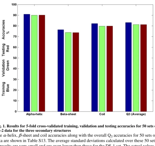
Classification of each residue in the test set is determined by the maximum votes received by one of the three secondary structure classes. The 5-fold cross-validation was carried out using different sets of hidden neurons which were limited in the range between 5% and 30% of the number of training samples. Of the 150 sets generated, 50 sets belonging to 10 cross-validation runs were selected where the number of hidden neurons was fewer than 10% of the number of training samples. These results are shown in Figures S13 and S14. Only these predictions are taken into consideration for further analysis. When all predictions (150 runs) were considered, the overall confidence level actually decreased by 0.3%, which shows that there is no significant gain from using a larger number of hidden neurons. Limiting the hidden neurons to be less than 10% of the number of training samples provides adequate and better generalization performance. The results for training, validation and testing are given in Tables S13 where the best test result of 83.4% is obtained when 573 hidden neurons are selected and the three values are within 2.5% of one another. The overall standard deviation is also very low at 0.7% over 50 sets of data. Table 2 shows the results of a 5-fold cross-validation study on DS-2, averaged over 50 runs. These results are illustrated in Figures 1 and S15. Overall (Q3) training, validation and testing accuracies are 83.2%, 81.2% and 81.3% respectively. Testing accuracies are highest for α-helix at 90.1% while β-sheet and coil show 73.7% and 79.9% respectively. Overall (Q3) values for sensitivity, specificity and MCC are 68.3%, 90.1% and 60.7% respectively. Coil has the highest sensitivity and MCC at 78.3% and 63.5% respectively, while α-helix has the highest specificity at 93.6%. The standard deviations are much lower for this study when compared to the DS-1 study, where the model was built using small proteins (Table S12). The SOV score is observed to be the highest for α-helix at 85.6% which is 5% less than its Q3 score of 90.1%. The overall SOV score is 78% which is only 1.8% less than other studies, as seen in Table 6. The β-sheet does better at 75.8% which is only 2% below its Q3 accuracy. Coil has the lowest SOV at 73.4% which is almost 6.5% less than its Q3 accuracy but still less than the 10% gap between the SOV score and coil accuracy values obtained for DS-1. These numbers are better and more uniform and closer to the individual accuracies and Q3 accuracy than the results seen earlier for DS-1. Table S14 and Figure S16 give the confidence levels for the predictions made using DS-2. This table and figure show the confidence level of predictions for the three secondary structures α-helix (H), β-sheet (E) and coil (C) along with the overall Q3 values obtained under a 5-fold cross-validation study using less than 800 hidden neurons. Percentage of residues predicted over ten different confidence levels are calculated (from 50% to 95%). α-helix (blue) has the highest confidence levels of predictions, where 94.3% of these residues are predicted with 50% confidence and at the other extreme, 84.5% are predicted with 95% accuracy. Similarly, for β-sheet (green), 82.4% of these residues are predicted with 50% confidence and at the other extreme, 62% are predicted with 95% accuracy. For coil (red), 87.7% of these residues are predicted with 50% confidence and at the other extreme, 69.4% are predicted with 95% accuracy. For overall (cyan) accuracies,

NIH-PA Author Manuscript

NIH-PA Author Manuscript

88.1% of all residues are predicted with 50% confidence and on the other extreme, 72.3% are predicted with 95% accuracy. In conclusion, we find that the results for the DS-2 study using a mix of small and large proteins from the CB513 provide better generalization and smaller standard deviations, but the overall prediction accuracy was slightly higher for the DS-1 study by about 3%. This might be due to the smaller size of the proteins used for that study. We find that the α-helix predictions are almost the same for both these studies while the prediction accuracies for β-sheet and coil are lower by 6.03% and 2.6% respectively, which contribute to the lower overall accuracy. The true test for the better model will be determined by how well the stored parameters do on independent test sets.

Results for DS-3

A set of 25 protein sequences (DS-3) known as switch proteins [54,55], each consisting of 56 amino acid residues provides a particularly interesting test set because the structures show a switch between a 3 helix bundle structure and a 4 beta strand plus 1 helix structure for a change of only one amino acid. These sequences are used in an independent study of the sensitivity of the present method to detect such a remarkable change from a single substitution. This provides an important test of the efficacy of the FLOPRED model. These proteins are listed in Table S15 and are detailed in section S1.5. The secondary structure for each of these proteins is predicted using the four models that were built earlier with DS-1 (averaged over 25 sets of data) and DS-2 (averaged over 150 sets of data). For each of these studies, results for obtained with different numbers of hidden neurons - (high (A) and low (B))were stored and used during testing to see how the number of hidden neurons used during modeling affects the test results. The parameters for all cross-validation runs on DS-1 and DS-2 were stored and used to predict the DS-3A and DS-3B sets separately. The results discussed here are averaged over all these runs for DS-3A and DS-3B which includes GA98 and GB98. We aim to see how well FLOPRED differentiates between these closely

homologous switching proteins which differ from each other so slightly but which

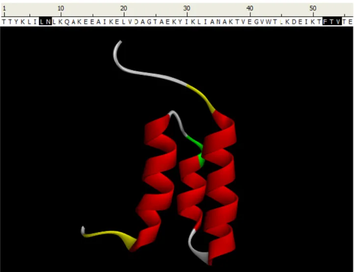
individually take on two different folds. These results are given in Table 3 and illustrated in Figures 4, S17 and S18. GA98 and GB98 proteins differ only by a single amino acid residue (L45Y) where the 45th residue leucine (L) is substituted for a tyrosine (Y), but these proteins have two different folds as described earlier and switch folds when a single amino acid is switched from one to the other. FLOPRED is able to differentiate between the two different folds (results are given here only for models built with DS-2) and predict the secondary structure of GA98 protein with 91.1% accuracy (51 correct predictions with 5 errors) as shown in Figure 2. (The figure and sequence shown are for the rendering of the GA95 protein since the PDB [1] file is available only for this protein, but the errors marked are for the prediction of the GA98). The erroneous predictions of the 5 residues are marked in yellow in the figure and in black on the sequence given above the figure, while the remaining 51 residues are predicted correctly and are shown in red for α-helix, white for coil and turns are shown in green. The 7th and 8th residues are erroneously predicted as α -helix instead of as coil, 52nd, 53rd residues are predicted as coil instead of as α-helix, while 54th residue is predicted as β-sheet instead of as coil. 43 out of 45 alpha-helix residues are predicted correctly and the two errors occur at the end of the α-helix, while the 4 errors in the coil residues occur on both ends of this protein. The GB98 protein has 56 residues [54, 55] and has a 4 beta strand plus 1 helix structure. FLOPRED predicts the secondary

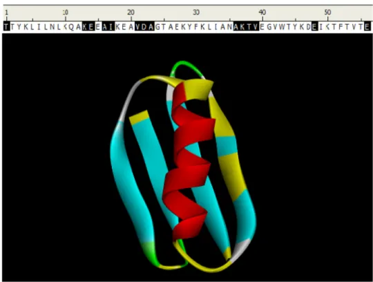
structure of this protein with 75% accuracy (42 correct predictions with 14 errors), as shown in Figure 3. (The figure and sequence shown are for the rendering of the GB95 protein since the PDB [1] file is available only for this protein, but the errors marked are for the prediction of the GB98). The erroneous predictions of the 14 residues are marked in yellow in the figure and in black on the sequence given above the figure, while the remaining 42 residues are predicted correctly and are shown in red for α-helix, blue for β-sheet. The 36th and 37th

α-helix residues are erroneously predicted as coil, and 23rd residue which is a β-sheet is

NIH-PA Author Manuscript

NIH-PA Author Manuscript

predicted as α-helix and all other erroneously predicted β-sheet residues are predicted as coil. The α-helix prediction accuracy is 84.3% (10 out of 12 residues) and β-sheet prediction accuracy is 72.3% (32 out of 44 residues) for an overall accuracy of 75%. For the GA proteins we have an overall QH accuracy of 95.5%, QC accuracy of 81 .8% and Q3 accuracy of 89.3% using the models built with DS-1A. When the same set of proteins are tested on DS-1B (where fewer hidden neurons were used), we obtain a QH accuracy of 84.4%, QC accuracy of 81.8% and Q3 accuracy of 83.9%. Thus, reducing the number of hidden neurons seems to lower the overall accuracy for GA proteins by 5.4% when they are tested on models built with small proteins. The biggest impact is on the accuracy of α-helix which drops by 6.7% while the coil accuracy stays the same for all models. The reduction in α-helix accuracy has a larger impact on the Q3 accuracy since there are 45 α-helix residues compared to only 11 coil residues. We get much higher results when the GA proteins are tested using the models built with DS-2. The QH, QC and Q3 accuracies are 97.8%, 81.8% and 94.6% for both models built with DS-2. Here the overall accuracies and α-helix accuracies are much higher while the accuracies for coil do not show any improvement when compared to the accuracies obtained on the models built with DS-1. Reducing the number of hidden neurons does not seem to have any effect overall for the GA proteins when the training models are built with a mix of small and large proteins.

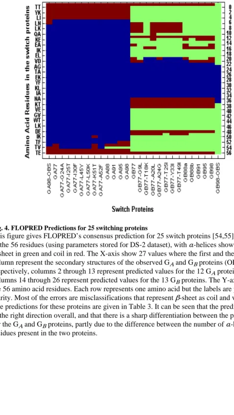
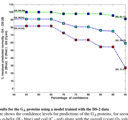
The consensus predictions are obtained using all the models that were built earlier with the DS-1 and DS-2 sets and are shown in Figures 4, S20 and S21 and in Table S15. This study also indicates that the confidence levels with which these predictions are made are higher when smaller number of hidden neurons are used. These results are illustrated in Figure 5, S16 and S19. For the GA proteins, we can see that 100% of α-helices are predicted with 65% confidence and 91.1% of the residues are predicted with 95% confidence. 81.8% of coil residues are predicted with 65% confidence and 27.3% of the residues are predicted with 95% confidence. Overall, 91.0% of GA proteins are predicted with 50% confidence and 59.2% of all residues are predicted with 95% confidence. For the GB proteins, we can see that 92.9% of α-helices are predicted with 50% confidence and 85.7% of the residues are predicted with 95% confidence. 88.1% of β-sheet residues are predicted with 50%

confidence and 38.1% of the residues are predicted with 95% confidence. Overall, 90.5% of GB proteins are predicted with 50% confidence and 61.9% of all residues are predicted with 95% confidence. The percentage of residues correctly predicted for the GA and GB proteins using the DS-2B data are given in Figures S20 and S21. The final predicted class for each residue is a consensus obtained after testing the residues using parameters from 25 models built with DS-1 and 150 models built with DS-2, whose parameters were stored after training and validation. Figure S20 shows the percentage of predictions (Y-axis) that were predicted correctly for each residue in GA proteins. The 56 residues are represented on the X-axis. We have observed that if the percentage of prediction falls below 39.6% then the predictions turn out to be erroneous. All the predictions above this line are correct. There are only three errors in the over-all prediction of the GA proteins when tested using the models built with DS-2B. (One of the predictions near the borderline which separates the correct predictions from the errors at the 40% mark, given in Figure S20, is also correct). Most interestingly, the 45th residue, in GA98 and GB98, that is a change in amino acid between leucine (L) and tyrosine (Y), is correctly predicted with 100% confidence in all the four studies, as shown in Figures 4, S20 and S21 and in Table S15. The consistency of the prediction of this switched residue indicates that FLOPRED is able to discern this subtle difference and correctly predict the residue’s secondary structure from its context even though the sequences differ very slightly, by only a single residue.

The higher accuracies for GA proteins can be attributed to the fact that 45 out of 56 residues belong to α-helix secondary structure. In contrast, the number of α-helix residues in GB protein is only 14 while the number of β-sheet residues is 42, and hence the contribution

NIH-PA Author Manuscript

NIH-PA Author Manuscript

from the α-helices in terms of overall accuracy is small. The SOV score for GA proteins are observed to be highest for coil at 99.4% compared to α-helix at 92.8% with an overall score of 93.9%. There is only one α-helix in this protein, and it spans 45 residues while there are only 11 coil residues on the two ends of this protein. The length and position of these secondary structure elements might bias the SOV score interpretations. These SOV scores were nevertheless better than those SOV scores obtained where the models had been trained on small proteins (DS-1), which had an overall score of only 26.3% (not shown in table) due to a fragmented alpha-helix prediction, although the Q₃ accuracy was misleadingly higher at 83.9%. The higher SOV score of 93.9% is obtained when the switch proteins are tested with models built from a mix of small and large proteins (DS-2) where the Q3 accuracy is better and closer at 94.6%, showing that it appears to be important to have a good mix of small and large proteins to train the model. Similarly, for the GB proteins, the QH, QE and Q3

accuracies are 85.7%, 71.4% and 75% for models built using DS-1A, while the accuracies are 78 .6%, 64.3% and 67.9% for QH, QE and Q3, respectively, when tested on models built using DS-1B. There is a 7.1% fall in accuracy for all three values which indicates that the GB protein predictions are sensitive to the number of hidden neurons used if tested with models where only small proteins were used. When the GB proteins are tested on models built with DS-2A, the accuracies are 85.7%, 69.1% and 73.2% for QH, QE and Q3, respectively, while the accuracies are 85.7%, 71.4% and 75% for QH, QE and Q3 when tested on models built with DS-2B. There is no change in the accuracy for α-helix while there is an increase of 2.4% accuracy for β-sheet and 1.8% increase in overall accuracy, when reduced number of hidden neurons are used for modeling. Hence, the reduction in hidden neurons seem to affect only the β-sheet accuracy slightly when models are built with small and large proteins and tested on the GB proteins. The results for switch proteins are shown in Figure 4. The predictions indicate that the first 8 and the last 3 residues of the GA proteins are coil (red) and the rest of them are α-helix (blue). For the GB proteins, residues 23 through 36 are α-helix (blue) while the rest of the residues are β-sheet (green). This figure shows that most of the errors are misclassifications of β-sheet (green) as coil and vice-versa, although some residues are misclassified as α-helix. The SOV score for GB proteins are observed to be highest for α-helix at 85.7%, which is the same as their individual accuracies compared to SOV for beta-sheet at only 69.9%, which is 2% lesser than its individual accuracy of 71.4%, while the overall SOV score of 74% is only 1% less than its Q3 accuracy of 75%. There are four β-sheets in this protein which span 42 residues while there are only 14 α-helix residues which are in the middle of this protein. These SOV scores are nevertheless better than for those SOV scores obtained with results where the models had been trained on small proteins (DS-1), where the overall score was only 21% due to a much fragmented alpha-helix SOV score of 52% and β-sheet score of only 17% (not shown in the table) although the Q3 accuracy was misleadingly higher at 70%. The higher SOV score of 74% was obtained when the switch proteins are tested with models built from a mix of small and large proteins (DS-2B with fewer hidden neurons), while the Q3 accuracy is slightly better and closer at 75%.

In conclusion, we see that the models built with only small proteins provide lower prediction accuracies while models built with training sets containing a homogenous mixture of small and large proteins yield better performance when tested on GA proteins, while GB proteins appear not seem to be very sensitive to the sizes of proteins used in the models and they give the same accuracies for both cases. These studies also show that it is important to have a good mix of small and large proteins to train the model for good generalization even if the protein has a larger number of residues belonging to one type of secondary structure element compared to others.

NIH-PA Author Manuscript

NIH-PA Author Manuscript

Results for DS-4

A set of 78 proteins (6605 residues) are selected using the PISCES culling server [41] with the criteria that they are less than 120 residues with a percentage identity less than 20%, resolution cutoff of 1.8 angstroms and an R-factor cutoff which is less than 0.3. These proteins are tested using the FLOPRED models built with DS-1 and DS-2. This is a highly diverse set and differs significantly from the switching proteins that are all very similar to one another and differ only by a few residues (Table S15). The proteins in DS-4 have less than 20% similarity with each other (Table S16). The same models that were used to test DS-3 are used to test DS-4, as described earlier and test results are averaged over all runs with DS-4. We aim to see whether FLOPRED can efficiently predict secondary structures when applied to this diverse set of proteins having less than 20% sequence identity and compare the results with those obtained for the more limited DS-3 set. The results for predictions of secondary structures for the DS-4 proteins are given in Table 4 and illustrated in Figure 6. This table gives the prediction accuracies for four independent studies

conducted with DS-4 proteins with four different models, DS-1A, DS-1B, DS-2A and DS-2B, where large (A) and small (B) numbers of hidden neurons are used in DS-1 and DS-2. When large (A) number of hidden neurons are used, they are limited to be between 5% and 30% of the number of training samples used. This number could be as high as 1560 for DS-1 and 2250 for DS-2. When smaller number of hidden neurons are used (B) they are limited to be between 5% and 11% of the number of training samples. This number could be as high as 425 for DS-1 and 760 for DS-2, depending on the number of residues present in the proteins selected for training the model. We observe that the accuracies for α-helices are highest for all sets compared to coil and β-sheet and Q3 accuracy is higher for the DS-2 than it is for DS-1 by almost 7%. Notably, the increase in accuracies for the DS-2 set originates from improved accuracies in β-sheet (11%) and coil (8%) and to a smaller (2%) extent in the

α-helix predictions. Overall the accuracies for these proteins are at 84.2% and 84.4% for the two subsets of DS-2 where a good mix of small and large proteins are used for model building and do not seem to be sensitive to the number of hidden neurons used, as observed previously for the switching proteins also. The SOV score is only 45.3% when tested on DS-1, while the corresponding Q3 accuracy is much higher at 77.8%. The SOV score improves significantly when tested on models built with the DS-2 model that has a mix of small and large proteins. The SOV score is highest for α-helix at 82.9%, 78.3% for β-sheet and 71.4% for coil, with an overall score of 76.9%, which is still 8% less than the Q3 accuracy of 84.4%. These results are illustrated in Figure 6. Average confidence levels for DS-4 using models built with DS-2 are given in Table 5 for each of the three secondary structures and overall Q3 values. These results are illustrated in Figure S22. α-helix has the highest confidence levels of prediction where 90.5% of these residues are predicted with 65% confidence and at the other extreme, 86.6% are predicted with 95% confidence. For β -sheet, 75.8% of these residues are predicted with 55% confidence and at the other extreme, 62.7% are predicted with 95% confidence. For coil, 81.5% of these residues are predicted with 55% confidence and at the other extreme, 66.6% are predicted with 95% confidence. For overall Q3 values 82.9% of all residues are predicted with 55% confidence and on the other extreme, 72.0% are predicted with 95% confidence. The actual values are given in Table 5. Finally, Figures S23 and S24 give an analysis of the number of residues predicted correctly for confidence levels from 5% through 95%. The final predicted class for each residue is a consensus obtained after testing the residues using parameters from 25 models built with DS-1 and 150 models built with DS-2, whose parameters were stored after training and validation. This histogram shows the number of residues (Y-axis) predicted correctly at different levels of percentage accuracy given on the X-axis. Out of 6605 residues, we can see that almost about 340 residues are predicted with 55% confidence and about 2700 residues are predicted with 95% accuracy and the remaining residues at different levels of confidence. In Figure S24, we can see that almost 100 residues are predicted within

NIH-PA Author Manuscript

NIH-PA Author Manuscript

a range of accuracies between 15% and 85% confidence and about 5000 residues are predicted with 95% accuracy.

Comparison of FLOPRED with other secondary structure prediction methods

We now compare FLOPRED DS-1 results with those studies in literature that use the CB513 dataset for secondary structure prediction (Table 6). All the methods that are listed include multiple sequence (evolutionary) information, to develop their models whereas we use information derived from protein sequences and knowledge-based potentials calculated using the CABS algorithm. Some of these studies also use very elaborate algorithms while our model uses only a single layer neural network with Particle Swarm Optimization. The overall Q3 training, testing and validation accuracies are 87.4%, 84.9% and 84.1% respectively. Except in one case, our average testing accuracy of 84.1% is higher than the accuracies found in literature. Our method achieves between 8.3% and 4.1% increase in Q₃ results compared for most previous methods and is only slightly below (1.4%) the CPM [31] method that has the highest Q₃ reported accuracy (85.6%), but CPM uses a much more elaborate algorithm to obtain this efficiency. CPM predicts protein secondary structure using a multi-layered approach which integrates several methods to produce the final results. One of our studies also achieves the highest accuracy of 85.7% when 1066 neurons are selected, but we have taken a conservative approach to limit the number of hidden neurons to be less than 11% of the number of training samples in order to achieve better generalization performance. Table 1 and Figure S11, gives the individual secondary structure accuracies for α-helix, β-sheet and coil. The training, testing and validation accuracies are the highest in this study for α-helix at 92.2%, 90.2% and 90.1% respectively. The training, testing and validation accuracies for β-sheet are 83.6%, 81% and 79.8% respectively while those for coil are 86.3%, 83.6% and 82.6% respectively. These results are higher compared to other results found in the literature (with one exception) as seen in Table 6. FLOPRED’s α-helix and β-sheet testing accuracies are 2.5% and 3.0% higher, while the accuracy for coil is 4.4% less compared to CPM. All other results for secondary structures cited in this table are less than the accuracies obtained by FLOPRED. Table 1 and Figure S12 also show the

sensitivity, specificity and Mathew’s correlation coefficient calculated from the 13 sets of selected results. Similarly, the other metrics seen in this table such as, 95.4% specificity for

α-helix, 80.7% sensitivity for coil and a Matthew’s correlation coefficient of 67.1% for coil are also higher for the FLOPRED DS-1 study compared to those found in the literature. These higher accuracies can be attributed to the learning capabilities of the ELM algorithm and the advanced optimization techniques offered by the PSO algorithms [37] that were used to tune the parameters of the neural network. For the DS-2 study, the α-helix testing

accuracies are still the highest compared to other studies while the β-sheet accuracies are lower only in comparison with those of CPM and DS-1 set. Coil accuracies do not fare so well compared to previous studies, and the overall accuracy is 4.3% lower than the CPM study and 2.9% lower than in the DS-1 study. The SOV scores are 77.6% for DS-1B set which is between 1.1% and 6.8% higher than the first four studies listed, 2.2% lesser than the CPM study, 1.4% lesser than the SPINE X study. The SOV scores for DS-2B are 78%, which is between 1 and 7% higher than the first four studies listed, 1.9% lesser than the CPM study and 1% lesser than the SPINE X study. We are unable to make similar

comparative studies for DS-3 and DS-4 with other studies in the literature since it is difficult to find a study which uses the same proteins. Hence we compare them only with one another. In comparing the results for the independent studies on DS-3 and DS-4 we see that predictions for α-helix structures do well in both these studies. These predictions are much higher for GA proteins at 97.8%, followed by 91.6% for DS-4 (6% lower) and only 75% for GB proteins (when lower number of hidden neurons are used and modeled using a mixture of small and large proteins). Similarly, the overall Q3 accuracies are higher for GA proteins at 94.6% followed by DS-4 at 84.4 (10% lower), and they are even lower for GB proteins at

NIH-PA Author Manuscript

NIH-PA Author Manuscript

75%. The higher accuracies for GA proteins can be attributed to the predominance of α -helices in the GA proteins. The accuracies obtained in tests on DS-4 are comparable with the cross-validation accuracies for DS-1 at 84.1%. DS-4 accuracies are higher than those obtained for DS-2 set by almost 3%. Notably, this increase came from improved accuracies in β-sheet (11%) and coil (8%) which might indicate that a good mix of big and small proteins in the training set can help to obtain better results for predicting β-sheet and coil secondary structures.

Conclusions

FLOPRED has performed evenly on small and large proteins from four different data sets, where three of these had only small proteins and the fourth one had a mixture of small and large proteins. So, FLOPRED gives somewhat better results for those proteins with

predominantly α-helix structures and lower accuracy for structures that have predominantly

β-sheet structures such as the GB proteins and it seems to do fairly well on a randomly selected set of proteins that have similar lengths but have a more homogenous mix of secondary structures. FLOPRED has SOV scores comparable to some of the best prediction servers available today. On the whole FLOPRED performs best when the proteins used for developing the computational model include a mixture of small and large proteins and a smaller number of hidden neurons is used. FLOPRED has good prediction capabilities for

α-helices but somewhat lower prediction accuracies for β-sheet and coil. We have also investigated the contribution of the twenty amino acids to the prediction accuracies which might be used to improve the results.

Supplementary Material

Refer to Web version on PubMed Central for supplementary material.

Acknowledgments

The algorithm for knowledge-based potentials data, was developed by members from the Kolinski [32] lab. We would like to thank Dr. John Orban for providing us with the sequences for the switching proteins. This work was supported by the National Institutes of Health grants R01GM081680, R01GM072014 and National Science Foundation grant IGERT-0504304.

References

1. Berman HM, Westbrook J, Feng Z, Gilliland G, Bhat TN, Weissig H, Shindyalov IN, Bourne PE. Nucleic Acids Res. 2000; 28:235. [PubMed: 10592235]

2. Chou PY, Fasman GD. Biochemistry. 1974:13, 222.

3. Garnier J, Osguthorpe DJ, Robson B. J Mol Biol. 1978; 1:97. [PubMed: 642007] 4. Garnier J, Gibrat JF, Robson B. Methods Enzymol. 1996:226, 540. [PubMed: 8791781] 5. Zvelebil MJ, Barton GJ, Taylor WR, Sternberg MJE. J Mol Biol. 1987; 195:957. [PubMed:

3656439]

6. Kloczkowski A, Ting KL, Jernigan RL, Garnier J. Proteins. 2002; 49:154. [PubMed: 12210997] 7. Salzberg S, Cost S. J Mol Biol. 1992; 227:371. [PubMed: 1404357]

8. Yi TM, Lander ES. J Mol Biol. 1993; 232:1117. [PubMed: 8371270] 9. Salamov AA, Solovyev VV. J Mol Biol. 1995; 247:11. [PubMed: 7897654] 10. Salamov VV, Solovyev AA. J Mol Biol. 1997; 268:31. [PubMed: 9149139]

11. Vapnik, VN. The Nature of Statistical Learning Theory (Information Science and Statistics). Springer-Verlag; New York: 2000.

12. Ward JJ, McGuffin LJ, Buxton BF, Jones DT. Bioinformatics. 2003; 19:1650. [PubMed: 12967961]

NIH-PA Author Manuscript

NIH-PA Author Manuscript

13. Qian N, Sejnowski TJ. J Mol Biol. 1988; 202:865. [PubMed: 3172241] 14. Rost B, Sander C. J Mol Biol. 1993; 232:584. [PubMed: 8345525] 15. Rost B. Methods Enzymol. 1996; 266:525. [PubMed: 8743704] 16. Cuff JA, Barton GJ. Proteins. 2000; 40:502. [PubMed: 10861942] 17. Jones D. J Mol Biol. 1999; 292:195. [PubMed: 10493868]

18. Rost B, Yachdav G, Liu J. Nucleic Acids Res. 2004; 32:W321. [PubMed: 15215403] 19. Eddy SR. Bioinformatics. 1998; 14:755. [PubMed: 9918945]

20. Kihara D. Protein Science. 2005; 14:1955. [PubMed: 15987894]

21. Madera M, Calmus R, Thiltgen G, Karplus K, Gough J. Bioinformatics. 2010; 26:596. [PubMed: 20130034]

22. Montgomerie S, Sundaraj S, Gallin W, Wishart D. BMC Bioinformatics. 2006; 301:301. [PubMed: 16774686]

23. Pollastri G, Martin A, Mooney C, Vullo A. BMC Bioinformatics. 2007; 8:201. [PubMed: 17570843]

24. Wang G, Zhao Y, Wang D. Neurocomputing. 2008; 72:262.

25. Malekpour SA, Naghizadeh S, Pezeshk H, Sadeghi M, Eslahchi C. Mathematical Biosciences. 2009; 217:145. [PubMed: 19046975]

26. Palopoli L, Rombo SE, Terracina G, Tradigo G, Veltri P. Information Fusion. 2009; 10:217. 27. Santiago-Gómez MP, Kermasha S, Nicaud JM, Belin JM, Husson F. J Mol Catal B-Enzym. 2010;

65:63.

28. Yang B, Wei H, Zhun Z, Huabin Q. Expert Syst Appl. 2009; 36:9000. 29. Zhou Z, Yang B, Hou W. Expert Syst Appl. 2010; 37:6381.

30. Babaei S, Geranmayeh A, Seyyedsalehi SA. Comput Meth and Prog Bio. 2010; 100:237. 31. Yang B, Wu Q, Ying Z, SH. Knowl-Based Syst. 2011; 24:304.

32. Kolinski A. ACTA Biochem Pol. 2004; 51:349.

33. Kennedy J, Eberhart RC. Particle Swarm Optimization. 1995 34. Fernández-Martínez JL, García-Gonzalo E. JAEA. 2008; 2008:15.

35. Fernández-Martínez JL, García-Gonzalo E, Fernández-Alvarez JP. IJCIR. 2008; 4:93. 36. García-Gonzalo E, Fernández-Martínez JL. P IC-CMS. 2009:1280–1290.

37. Fernández-Martínez JL, García-Gonzalo E. PIJCCI/ICNC. 2010:237–242.

38. Fernández-Martínez JL, García-Gonzalo E. IEEE Trans Evol Comput. 2011; 15:405. 39. Rost B, Sander C. Proteins. 1994; 20:216. [PubMed: 7892171]

40. Zemla A, Venclovas, Fidelis K, Rost B. Proteins: Struct, Funct, Bioinf. 1999; 34:220. 41. Wang G, Dunbrack RLJ. Bioinformatics. 2003; 19:1589. [PubMed: 12912846]

42. Orengo CA, Michie AD, Jones DT, Swindells JM, Thornton MB. Structure. 1997; 5:1093. [PubMed: 9309224]

43. Huang GB, Zhu QY, SCK. Neurocomputing. 2006; 70:489.

44. Saraswathi S, Jernigan RL, Koliniski A, Kloczkowski A. P IJCCI/ICNC. 2010:370–375. 45. Suresh S, Saraswathi S, Sundararajan N. EAAI. 2010; 23:1149.

46. Needleman SB, Wunsch CD. J Mol Biol. 1970; 48:443. [PubMed: 5420325]

47. Henikoff S, Henikoff J. Proc Natl Acad Sci U S A. 1992; 89:10915. [PubMed: 1438297] 48. Sander C, Schneider R. Proteins. 1991; 9:56. [PubMed: 2017436]

49. Kabsch W, Sander C. Biopolymers. 1983; 22:2577. [PubMed: 6667333] 50. Silva PJ. Proteins. 2008; 70:1588. [PubMed: 17918727]

51. Saraswathi S, Suresh S, Sundararajan N, Zimmermann M, Nilsen-Hamilton M. IEEE ACM T Comput Bi. 2011; 8:452.

52. Fernández-Martínez JL, García-Gonzalo E. Swarm Intell : Spec Publ PSO. 2009; 3:245.

53. Fahnestoc S, Alexander P, Nagle J, Filpula D. J Bacteriol. 1986; 167(3):870. [PubMed: 3745123] 54. Alexander PA, He Y, Chen Y, Orban J, Bryan PN. Proc Natl Acad Sci U S A. 2009; 106(50):

21149. [PubMed: 19923431]

NIH-PA Author Manuscript

NIH-PA Author Manuscript

55. Bryan PN, Orban J. Curr Opin Struct Biol. 2010; 20(4):482. [PubMed: 20591649]

56. Faraggi E, Zhang T, Yang Y, Kurgan L, Zhou Y. J Comput Chem. 2012; 33(3):259. [PubMed: 22045506]

NIH-PA Author Manuscript

NIH-PA Author Manuscript

Fig. 1. Results for 5-fold cross-validated training, validation and testing accuracies for 50 sets of DS-2 data for the three secondary structures

The α-helix, β-sheet and coil accuracies along with the overall Q3 accuracies for 50 sets of data are shown in Table S13. The average standard deviations calculated over these 50 sets of results are very small and are even lower than those for the DS-1 set. The actual values are given in Table 2 and are discussed further in the results section for DS-2.

NIH-PA Author Manuscript

NIH-PA Author Manuscript

Fig. 2. FLOPRED Predictions for G_A98 protein

The GA98 protein has 56 residues [54, 55] and has a 3 helix bundle structure. FLOPRED predicts the secondary structure of this protein with 91.1% accuracy (51 correct predictions with 5 errors). The erroneous predictions of the 5 residues are marked in yellow in the figure and marked in black on the sequence given above the figure, while the remaining 51

residues are predicted correctly and are shown in red for α-helix, white for coil and the turns are shown in green.

NIH-PA Author Manuscript

NIH-PA Author Manuscript

Fig. 3. FLOPRED Predictions for G_B98 protein

The GB98 protein has 56 residues [54, 55] and has a 4 beta strand plus 1 helix structure. FLOPRED predicts the secondary structure of this protein with 75% accuracy (42 correct predictions with 14 errors). The erroneous predictions of the 14 residues are marked in yellow in the figure and in black on the sequence given above the figure, while the remaining 42 residues are predicted correctly and are shown in red for α-helix, blue for β -sheet and the turns are shown in green. (Although some of the coloring is rendered in white representing coil, this protein has no residues classified as coil).

NIH-PA Author Manuscript

NIH-PA Author Manuscript

Fig. 4. FLOPRED Predictions for 25 switching proteins

This figure gives FLOPRED’s consensus prediction for 25 switch proteins [54,55] for each of the 56 residues (using parameters stored for DS-2 dataset), with α-helices shown in blue,

β-sheet in green and coil in red. The X-axis show 27 values where the first and the last column represent the secondary structures of the observed GA and GB proteins (OBS) respectively, columns 2 through 13 represent predicted values for the 12 GA proteins and columns 14 through 26 represent predicted values for the 13 GB proteins. The Y-axis shows the 56 amino acid residues. Each row represents one amino acid but the labels are paired for clarity. Most of the errors are misclassifications that represent β-sheet as coil and vice-versa. The predictions for these proteins are given in Table 3. It can be seen that the predictions are in the right direction overall, and that there is a sharp differentiation between the predictions for the GA and GB proteins, partly due to the difference between the number of α-helix residues present in the two proteins.

NIH-PA Author Manuscript

NIH-PA Author Manuscript

Fig. 5. Results for the G_A proteins using a model trained with the DS-2 data

This figure shows the confidence levels for predictions of the GA proteins, for secondary structures α-helix (H - blue) and coil (C - red) along with the overall (cyan) Q₃ values obtained under an independent study using DS-2. These results are discussed further in the results section.

NIH-PA Author Manuscript

NIH-PA Author Manuscript

Fig. 6.

Results of an independent study of the DS-4 proteins on DS-1 and DS-2 data using a wide range of hidden neurons This figures shows that the α-helix (H - blue) accuracies are higher than those for β-sheet (E - green) and coil (C - red) for all four sets. The overall accuracy (cyan - Q3) is higher for the DS-2A and DS-2B sets and there seems to be less sensitivity to the number of hidden neurons used for models based on DS-2A and DS-2B, since there is only a 0.17% difference in accuracy between these results. Predictions using models built with a mix of small and large proteins perform better than those predictions which were obtained using models which were built using data consisting of only small proteins (DS-1). The actual values are given under Table 4 and are discussed further in the results section for DS-4.

NIH-PA Author Manuscript

NIH-PA Author Manuscript

NIH-PA Author Manuscript

NIH-PA Author Manuscript

NIH-PA Author Manuscript

Table 1

Test results for DS-1 from a 5-fold cross-validation study. 3800 to 4250 residues were used for the training model, 1100 to 1300 residues were used for validation and the remaining 1200 to 1400 residues were used for testing. (Different number of residues are chosen for each set during random selection of proteins). These results are illustrated in Figures S10, S11, and S12. and are further discussed under results for DS-1, where the numbers given are percentages. Metrics

α -helix β -sheet Coil Overall a Stdev Training 92.2 83.6 86.3 87.4 0.6 Validation 90.2 81.0 83.6 84.9 1.0 Testing 90.1 79.8 82.6 84.1 1.0 SOV b 89.6 76.4 72.2 77.6 – Sensitivity 64.2 68.8 80.7 71.2 4.1 Specificity 95.4 91.2 86.2 91.0 1.4 MCC c 65.3 62.5 67.1 65.0 2.6

a Overall scores are the Q

3

scores, the average accuracy of prediction for all three secondary structures.

NIH-PA Author Manuscript

NIH-PA Author Manuscript

NIH-PA Author Manuscript

Table 2

Testing results for DS-2 for a 5-fold cross-validation study, averaged over 50 runs. Approximately 50, 000 residues were used for the training model, 13, 000 residues for validation and the remaining 13, 000 residues were used for testing. These results are illustrated in Figures 1 and S15 and are further discussed under the results section for DS-2. Metrics

α -helix β -sheet Coil Overall Stdev Training 91.0 76.4 82.3 83.2 1.0 Validation 90.0 73.9 79.8 81.2 0.8 Testing 90.1 73.7 79.9 81.3 0.7 SOV 85.6 75.8 73.4 78.0 – Sensitivity 68.4 58.2 78.3 68.3 2.5 Specificity 93.6 91.6 85.0 90.1 1.0 MCC 64.9 53.9 63.5 60.7 1.6