Application of a hybrid of least square support vector machine and artificial bee colony for building load forecasting

78: 6–2 (2016) 91–96 | www.jurnalteknologi.utm.my | eISSN 2180–3722 |

Jurnal

Teknologi

Full Paper

A

PPLICATION OF A HYBRID OF LEAST SQUARE

SUPPORT VECTOR MACHINE AND ARTIFICIAL BEE

COLONY FOR BUILDING LOAD FORECASTING

Mohammad Azhar Mat Daut

a,b

_{, Mohammad Yusri Hassan}

a,b*

_,

Hayati Abdullah

a,c

_{, Hasimah Abdul Rahman}

a,b

_{, Md Pauzi}

Abdullah

a,b

_{, Faridah Hussin}

a,b

a

_{Centre of Electrical Energy Systems (CEES), Institute of Future}

Energy, Universiti Teknologi Malaysia (UTM), 81310 Johor Bahru,

Johor, Malaysia

b

_{Faculty of Electrical Engineering, Universiti Teknologi Malaysia}

(UTM), 81310 Johor Bahru, Johor, Malaysia

c

_{Faculty of Mechanical Engineering, Universiti Teknologi Malaysia}

(UTM), 81310 Johor Bahru, Johor, Malaysia

Article history Received 04 June 2015 Received in revised form 27November 2015 Accepted 01January 2016

*Corresponding author

[email protected]

Graphical abstract

Abstract

Accurate load forecasting is an important element for proper planning and management of electricity production. Although load forecasting has been an important area of research, methods for accurate load forecasting is still scarce in the literature. This paper presents a study on a hybrid load forecasting method that combines the Least Square Support Vector Machine (LSSVM) and Artificial Bee Colony (ABC) methods for building load forecasting. The performance of the LSSVM-ABC hybrid method was compared to the LSSVM method in building load forecasting problems and the results has shown that the hybrid method is able to substantially improve the load forecasting ability of the LSSVM method.

Keywords: Load forecasting, least square support vector machine, artificial bee

colony

© 2016 Penerbit UTM Press. All rights reserved

1.0 INTRODUCTION

The increase in production cost in the power generating industry requires a consideration of more economical and reliable operation including the accuracy of load forecasting. Accurate load forecasting is essential to avoid a mismatch in load from happening.

Many research studies have been published in the literature on load forecasting using conventional methods such as stochastic time series [1] and multiple regression [2]. Currently, the most widely used involves the use of Artificial Intelligence (AI) methods. Some examples include Artificial Neural Network (ANN) and Support Vector Machine (SVM) [3, 4] methods. These

AI methods are able to capture non-linear relationships but they face over-fitting issues as discussed in various research studies [5, 6]. To this end, the hybrid methods are necessary in order to improve the performance of load forecasting.

The Least Square Support Vector Machine (LSSVM) [7] has proven to be a useful method for hybrid purposes. LSSVM has the benefits of Structural Risk Minimization (SRM) from its unique structure, namely the Support Vector Machine (SVM) [8]. The LSSVM is intended to minimize the upper bound generalization error as opposed to the training error as applied in the Empirical Risk Minimization (ERM). Thus, LSSVM is less uncovering with the over-fitting issue when compared

with other ANN methods [9]. LSSVM is also suitable for problems with restricted information [10].

Current studies in the hybridization of LSSVM with optimization algorithm, especially with Evolutionary Computation (EC) algorithm showed some potential in improving the performance of load forecasting. Among the EC calculations, Particle Swarm Optimization (PSO) [11] and Ant Colony Optimization (ACO) [12] are considered as having the most potential because of its application in the field of load forecasting. The PSO also has been used in some recent work [13].

In recent years, the utilization of honey bees based algorithm, in particular Artificial Bee Colony (ABC) [14] can be seen as having significant potential when compared to current optimization algorithms. When compared with the PSO and ACO, the ABC involves less control parameters and basic mathematical calculations. These features have resulted in its application in more extensive optimization problems.

The combination of LSSVM and ABC methods has been proposed in this study to improve the performance of load forecasting. In this study, the role of LSSVM is to train the actual load data which will be then be used for forecasting. The difference between the actual and the forecasted load data will be used to evaluate the performance accuracy. The result from the LSSVM will then be incorporated with the ABC algorithm. The role of the ABC algorithm is to find the local minimum for the results.

The remaining section of this paper is organized as follows: a brief description of the experimental methodis presented in section 2, the experiment and discussion is described in section 3 and the conclusion will be given in section 4.

2.0 EXPERIMENTAL

This section introduces the fundamental of Least Square Support Vector Machine and Artificial Bee Colony in terms of their theories and concepts.

2.1 Least Square Support Vector Machine

For nonlinear regression, given a training set of N points



x

_i

,

y

_i



with the input values,

x

_iand the output values,

y

_ithe aim is to obtain a model of the structure using equation 1 below [15]:

i i T

e

b

x

w

x

y

(

)





(

)





(1)

where is the weight vector,

b

is the bias and

e

_i is the blunder between the genuine and anticipated yield at the

i

_thtest point. The data,

x

_i and yield,

y

 

x

are explained in Section 5. The coefficient vector

w

and

b

can be obtained using the equations given below [15]:









N i i T

e

w

w

e

w

J

e

b

w

1 2

2

1

2

1

)

,

(

,

,

min



(2)

Subject to the equality constraints

N

i

e

b

x

w

y

_i



T



(

_i

)





_i

,



1

,

2

,....,

Applying the Lagrange multiplier to (2) yields:



















N i i i i T i

w

x

b

e

y

e

w

J

e

b

w

L

1

)

(

)

,

(

)

;

,

,

(







(3)

where



_iare Lagrange multipliers,



is the regularization parameter which adjusts the unpredictability of the LSSVM model, i.e. y(x), and the training error. Separating (3) with

w

,

b

,

e

_i and



_i the Karush-Kuhn-Tucker (KKT) conditions for optimality of this issue can be obtained by setting all subordinates equivalent to zero, as expressed in the followings:

 















N i i i

x

w

w

L

1

0



















N i i

b

L

1

0

0



i i i

e

e

L

_

_

_

_

_





0

 

0

0









_







i i i T i

y

e

b

x

w

L

_



(4) i = 1,2,…,N

By eliminating

w

and

e

_i , the optimization problem can be transformed into the following linear equation:



















































y

I

b

T v v

0

1

1

0





(

5)

TheLSSVM model for regression in (1) becomes:









N i i i

K

x

x

b

x

y

1

)

,

(

)

(



(6)

where



and

b

are from equation (5). In (6), there are a few available kernel functions

K



x

,

x

_i



, to be specific Radial Basis Function (RBF) kernel, Multilayer Perceptron (MLP) kernel or quadratic kernel. In this study, the RBF portion is utilized. It is expressed as:

2 2 2

)

,

(

 i x x i

e

x

x

K





(7) where



2

is a tuning parameter which is connected with RBF part. Another tuning parameter, which is regularization parameter,



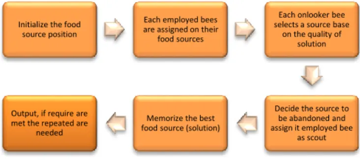
can be seen in (2) 2.2 Artificial Bee Colony

Artificial Bee Colony (ABC) is one of the methods in the Swarm Intelligence family. The ABC concept was introduced by Karaboga and Basturk [16], inspired from the behaviour of honey bee searching for food. The ABC has been compared with other algorithms for unconstrained and constrained problems [16]. The ABC algorithm has also been used in machine learning by training the neural network on classification [17] and clustering techniques [18]. The basic steps in the ABC algorithm is given in Fig. 1 [16].

Figure 1 Basic Step of ABC

In the ABC algorithm, two important elements are the food source and the amount of nectar. This food source represents the possible solution for the optimization problem while the amount of nectar is for the fitness value of the associated solution. The group bees in this algorithm can be categorized into three; employed, onlooker and scout bees. The function of the employed bee is to determine the food source from the neighbourhood and share their food with the onlooker bees. Then, the onlooker bees will select the food source. Increased in the number of nectar will increase the probability of selection [14]. The source will then be abandoned and the employed bee will become a scout and starts to search for a new food source randomly.

In the initialization stage, the population of food source will be generated randomly with a range of variable boundaries by using Eq. 8.

 



max min



min

1

,

0

_{j j} j ij

x

rand

x

x

x







(8)

where

i

represent the

i

_thfood source number and j is the optimization variable associated with the

i

_th food source. For the quality of the solution (fitness), the nectar amount will be evaluated according to Eq. 9



































0

if

0

if

)

(

1

)

1

(

1

i i i i i

f

f

f

abs

f

fitness

(9)

where fi is the cost associated with solution xi. . Then,

each employed bee will search for the new food source within the neighborhood which is already in the memory. The new food source will evaluated according to Eq. 10.



ij kj



ij ij ij

x

x

x

v









(10)

where j is a random optimization variable in the range of [1, D]. K is the randomly selected food source which is different from i, a uniformly distributed real number in the range [-1, 1] and D is a non-negative number. The next step will involve the solution weighting. In the solution weighting, each onlooker will select the higher probability by using Eq. 11.





_SN i j i i

fit

fit

p

(11)

where fiti is the fitness of the solution. SN is the

number of food source position. After all employed bees exploit a new solution and the onlooker bees are allocated the food source, if the food number is not being improved, it is abandoned and the employed bees with associated with which becomes a scout and make a random search according to Eq. 12.



max min



min d d d id

x

r

x

x

x







(12)

where

r

is a random real number within a range of [0,1]. min

d

x

and max d

x

is the boundaries in the

d

_th

dimension of the problem space.

3.0 RESULTS AND DISCUSSION

This section covers the data description and evaluation criteria for building load forecasting.

Initialize the food source position

Each employed bees are assigned on their

food sources

Each onlooker bee selects a source base

on the quality of solution

Decide the source to be abandoned and assign it employed bee

as scout Memorize the best

food source (solution) Output, if require are

met the repeated are needed

3.1 Data Description

The performance of the proposed method has been implemented and tested by using the dataset of input which include the weather, holidays, humidity, and actual hourly load. The output variable is the daily usage of the building consumer for two years ahead.

3.2 Evaluation Criteria

In this study, two evaluation criteria have been used as the measurement for forecasting performance which are the Means Absolute Percentage Error (MAPE) and the Means Absolute Error (MAE) [16]. Both parameters interpret the generalization capability of the model in making predictions. The definition is given in equations (13) and (14).

100

1

1

x

A

F

A

N

MAPE

N t t t t

_











_





 (13)









N i t t

A

F

N

MAE

1

1

(14) Where t=1,2,…,x At = actual values Ft = forecasted value N = Number of test data 3.2 Empirical Result

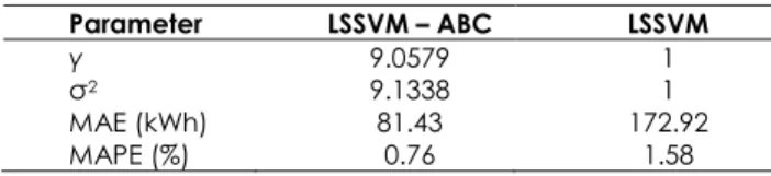
For analysis purposes, the results of proposed LSSVM-ABC were compared to those of the standard LSSVM. The results in Table 1 shows that the value of



and



2

produced by the LSSVM-ABC are 9.0579 and 9.1338 respectively. Using this hybrid method, the average of MAPE and MAE produced by the proposed method was 0.76 % and 81.43 kWh respectively, which has a lower value of MAPE compared to the LSSVM which resulted in the values of MAPE and MAE as 1.58% and 172.92 kWh respectively. The LSSVM with the small value of



2_{has resulted in over-fitting issues which}

consequently affects its forecasting capability.

Table 1 Building load forecasting

Parameter LSSVM – ABC LSSVM

γ 9.0579 1

σ2 _{9.1338 1}

MAE (kWh) 81.43 172.92 MAPE (%) 0.76 1.58

Table2 Actual and forecasted Load

Year Month _{Load (W)} Actual

ABC – LSSVM LSSVM Forecasted Load (W) MAE (Wh) MAPE (%) Forecasted Load (W) MAE (Wh) MAPE (%) 2008 January 11750534 11716457.76 34076.24 0.29 11765323.14 14789.14 0.13 February 10876512 10900022.25 23510.25 0.22 10906455.91 29943.91 0.27 March 11002037 10986681.38 15355.62 0.14 11033700.16 31663.16 0.29 April 9813955 9762765.242 51189.76 0.52 9875774.07 61819.07 0.63 May 9895937 9840586.922 55350.08 0.56 10003003.15 107066.15 1.07 June 11337827 11203100.47 134726.53 1.19 11009334.7 328492.30 2.90 July 13021300 12914686.38 106613.62 0.82 12523826.14 497473.86 3.82 August 11569470 11591649.03 22179.03 0.19 11530880.19 38589.81 0.33 September 10615976 10670837.19 54861.19 0.51 10687686 71710.00 0.67 October 10185148 10205357.94 20209.94 0.20 10223812.89 38664.89 0.38 November 10296718 10358363.85 61645.85 0.60 10412235.87 115517.87 1.11 December 11388228 11482600.25 94372.25 0.82 11441794.8 53566.80 0.47 2009 January 12004539 12163765.16 159226.16 1.31 12088114.55 83575.55 0.69 February 10143498 10331947.81 188449.81 1.82 10329076.55 185578.55 1.80 March 10539960 10732926.73 192966.73 1.80 10760175.4 220215.40 2.05 April 9515010 9628901.107 113891.11 1.18 9873726.655 358716.65 3.63 May 9663171 9742140.314 78969.31 0.81 10046374.22 383203.22 3.81 June 9960139 10003667.37 43528.37 0.44 10181161.91 221022.91 2.17 July 11290902 11364527.93 73625.93 0.65 11394635.71 103733.71 0.91 August 12556713 12510067.52 46645.48 0.37 11999350.56 557362.44 4.44 September 9889642 9990348.245 100706.25 1.01 10107619.32 217977.32 2.16 October 10004781 10087033.56 82252.56 0.82 10191473.22 186692.22 1.83 November 9749530 9853885.634 104355.63 1.06 9912421.309 162891.31 1.64 December 11524993 11620626.85 95633.85 0.82 11604732.02 79739.02 0.69

Figure 2 Comparison of MAPE for the two models

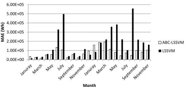
Figure 3 Comparison of MAE for the two models

The forecasted results using these two models are shown in Table 2. The actual load values and percentage error for each model are also shown in the table. It can be seen from Table 2 and Table 3, that the accuracy of the ABC-LSSVM model is better than the LSSVM model. Figure 2 and Figure 3 show the percentage error for each month for both models. From Figure 2, it can be seen that the MAPE of the ABC-LSSVM model is better than the LSSVM model. Figure 3 shows a comparison of the MAE between the actual and forecasted data.

4.0 CONCLUSION

This paper presents a hybrid method for LSSVM, which was incorporated with the ABC algorithm. The introduction of the ABC algorithm in this study has improved the performance of load forecasting by the LSSVM method. The results presented in this study for a building case study show that the forecasted value using the proposed hybrid method is very close to the actual value. It can be concluded that the ABC algorithm has significantly improved the performance of the LSSVM method and has the potential to be used for accurate building load forecasting.

0.00E+00 1.00E+05 2.00E+05 3.00E+05 4.00E+05 5.00E+05 6.00E+05 M A E (Wh ) Month ABC-LSSVM LSSVM 0.00 0.50 1.00 1.50 2.00 2.50 3.00 3.50 4.00 4.50 5.00 M A P E (% ) Month ABC-LSSVM LSSVM

Acknowledgement

This work was supported by the Ministry of Education Malaysia, and Universiti Teknologi Malaysia through the Research University Grant (GUP) vot 07H57.

References

[1] Pappas S. S., EkonomouL., KaramousantasD. C., ChatzarakisG. E., KatsikasS. K., and LiatsisP. 2008. Electricity demand loads modeling using AutoRegressive Moving Average (ARMA) Models.

Energy, 33(9): 1353-1360.

[2] Tao H., PuW., and WillisH. L. 2011. A Naive Multiple Linear Regression Benchmark For Short Term Load Forecasting. in Power and Energy Society General Meeting, 2011

IEEE. 1-6.

[3] Dong B., CaoC., and LeeS. E. 2005. Applying Support Vector Machines To Predict Building Energy Consumption In Tropical Region," Energy and Buildings. 37(5): 545-553.

[4] González P. A. and ZamarreñoJ. M. 2005. Prediction Of Hourly Energy Consumption In Buildings Based On A Feedback Artificial Neural Network. Energy and

Buildings. 37(6): 595-601.

[5] Foucquier A., RobertS., SuardF., StéphanL., and JayA. 2013. State Of The Art In Building Modelling And Energy Performances Prediction: A Review. Renewable and

Sustainable Energy Reviews. 23(7): 272-288.

[6] Lazos D., SproulA. B., and KayM. 2014. Optimisation Of Energy Management In Commercial Buildings With Weather Forecasting Inputs: A Review. Renewable and

Sustainable Energy Reviews. 39(11): 587-603.

[7] Samsudin P. S. R. and ShabriA. 2011. River Flow Time Series Using Least Squares Support Vector Machines.

Hydrology and Earth System Sciences. 18.

[8] Vapnik V. N. 1995. The Nature Of Statistical Learning

Theory: Springer-Verlag New York, Inc.

[9] Ji-yong S., Xiao-boZ., Xiao-weiH., Jie-wenZ., YanxiaoL., LiminH. et al. 2013. Rapid Detecting Total Acid Content And Classifying Different Types Of Vinegar Based On Near Infrared Spectroscopy And Least-Squares Support Vector Machine. Food Chemistry. 138: 192-199.

[10] WangX., ChenJ., LiuC. and PanF. 2010. Hybrid Modeling Of Penicillin Fermentation Process Based On Least Square Support Vector Machine. Chemical Engineering Research and Design. 88: 415-420.

[11] Gong Q., LuW., GongW., and WangX. 2014. Short-Term Load Forecasting of LSSVM Based on Improved PSO Algorithm. in Pattern Recognition. S. Li, C. Liu, and Y. Wang, Eds., ed: Springer Berlin Heidelberg, 483: 63-71.

[12] Sheikhan M. and MohammadiN. 2012. Neural-Based Electricity Load Forecasting Using Hybrid of GA and ACO for Feature Selection. Neural Computing and

Applications. 21: 1961-1970.

[13] Shang Y. and BouffanaisR. 2014. Influence Of The Number Of Topologically Interacting Neighbors On Swarm Dynamics. Sci. Rep.4.

[14] Karaboga D. 2005. An idea Based On Honey Bee Swarm for Numerical Optimization.

[15] SuykensJ. A. K., GestelT. V., BrabanterJ. D., MoorB. D. and VandewalleJ. 2011.LS-SVMlab Toolbox User’s

Guide.

[16] Karaboga D. and BasturkB. 2007. A Powerful And Efficient Algorithm For Numerical Function Optimization: Artificial Bee Colony (ABC) Algorithm .Journal of Global

Optimization. 39: 459-471.

[17] Bullinaria J. and AlYahyaK. 2013. Artificial Bee Colony Training of Neural Networks," in Nature Inspired

Cooperative Strategies for Optimization (NICSO 2013).

G. Terrazas, F. E. B. Otero, and A. D. Masegosa, Eds., ed: Springer International Publishing. 512: 191-201.

[18] Karaboga D. and Ozturk C. 2011. A novel clustering approach: Artificial Bee Colony (ABC) Algorithm.