Computational Methods for the Analysis of Single-Cell RNA-Seq Data

(1)

Masthead Logo

University of Connecticut

OpenCommons@UConn

Doctoral Dissertations University of Connecticut Graduate School

4-26-2019

Computational Methods for the Analysis of

Single-Cell RNA-Seq Data

Marmar Moussa

University of Connecticut - Storrs, [email protected]

Follow this and additional works at:https://opencommons.uconn.edu/dissertations Recommended Citation

Moussa, Marmar, "Computational Methods for the Analysis of Single-Cell RNA-Seq Data" (2019).Doctoral Dissertations. 2135.

(2)

Computational Methods for the Analysis of

Single-Cell RNA-Seq Data

Marmar Moussa, Ph.D. University of Connecticut, 2019

Single cell transcriptional profiling is critical for understanding cellular heterogeneity and identification of novel cell types as well as for studying growth and development of tissues and tumors. Leveraging the recent advances in single cell RNA sequencing (scRNA-Seq) technology requires novel methods that are robust to high levels of tech-nical and biological noise and scale to datasets of millions of cells. In this work, we address several challenges in the analysis work-flow of scRNA-Seq data: First, we pro-pose novel computational approaches for unsupervised clustering scRNA-Seq data based on the Term Frequency - Inverse Document Frequency (TF-IDF) transformation that has been successfully used in the field of text analysis. For this part, we present empirical experimental results showing that TF-IDF methods consistently outperform commonly used scRNA-Seq clustering approaches. Second, we study the so called ‘drop-out’ ef-fect that is considered one of the most notable challenges in single cell RNA-Seq data analysis, where only a fraction of the transcriptome of each cell is captured. The ran-dom nature of drop-outs, however, makes it possible to consider imputation methods as means of correcting for drop-outs. In this part we study some existing scRNA-Seq im-putation methods and propose a novel iterative imim-putation approach based on efficiently computing highly similar cells. We then present the results of a comprehensive assess-ment of existing and proposed methods on real scRNA-Seq datasets with varying per cell sequencing depth. Third, we present a computational method for assigning and/or ordering cells based on their cell-cycle stages from single-cell transcriptome data. And finally, we present a web-based interactive computational work-flow for the analysis and visualization of single-cell RNA-seq data.

(3)

Computational Methods for the Analysis of

Single-Cell RNA-Seq Data

Marmar Moussa

M.Sc., Alexandria University, 2004

M.Sc., University of Connecticut, 2018

A Dissertation

Submitted in Partial Fulfillment of the Requirements for the Degree of

Doctor of Philosophy at the

University of Connecticut 2019

(4)

Approval Page

Doctor of Philosophy Dissertation

Computational Methods for the Analysis of Single-Cell RNA-Seq Data

Presented by Marmar Moussa, B.Sc., M.Sc. Major Advisor Ion I. M˘andoiu Associate Advisor Mukul S. Bansal Associate Advisor Sheida Nabavi University of Connecticut 2019

(5)

Acknowledgements:

First and foremost I would like to thank my supervisor, Professor Ion M˘andoiu, for his guidance and support that he provided me throughout the past years. He taught, challenged and advised! A great model of support that I was extremely lucky to enjoy during my time as his student. There are not enough words to thank him; he will always have my deepest gratitude.

I would also like to thank Professor Steven A. Demurjian for his help and support, without him I would not have started this program in the first place.

Additionally, I would like to thank my thesis committee Professor Mukul Bansal and Professor Sheida Nabavi for their time, advice, and insightful comments. I would also like to extend my thanks to Professor Reda Ammar and Professor Sanguthevar Rajasekaran for their support and to the CSE Department especially Rebecca Randazzo and Joy Billion for their help throughout the program.

I must express my gratitude to Ahmad for his encouragement to start this program and for Laila who was my constant light throughout the years. She endured countless hours listening to my research obsessions.

Finally, I would like to give all my appreciation, love, and gratitude to Soheir, Moemen, Mayada, Maaly, and the great Reda Moussa for their constant belief in me and their unconditional support, they were, still are, and will always be my best friends and greatest allies.

(6)

Chapter 1 Introduction

The recent advances in single cell RNA sequencing (scRNA-Seq) technologies promise to unveil novel cell types and uncover subtle regulatory processes that are undetectable by analyzing bulk samples. Currently, droplet-based technologies such as the Chromium Megacell commercialized by 10x Genomics can quickly and inexpensively generate scRNA-Seq expression profiles for up to millions of cells. However, the sequencing depth of each cell in such datasets is typically very low, resulting in many missing gene expression levels. The large amounts of data and high levels of noise render many unsupervised clustering methods developed for bulk gene expression data [24] unusable, prompting the devel-opment of a new generation of computational methods tailored for single cell RNA-Seq data analysis. Single cell transcriptional profiling is critical for understanding cellular heterogeneity and identification of novel cell types as well as for studying growth and development of tissues and tumors. Leveraging the recent advances in single cell RNA sequencing (scRNA-Seq) technology requires novel computational methods that are ro-bust to high levels of technical and biological noise and scale to datasets of millions of cells.

In this work, we address several challenges in the analysis work-flow of scRNA-Seq data: First, we propose novel computational approaches for unsupervised clustering of scRNA-Seq data based on the Term Frequency - Inverse Document Frequency (TF-IDF) (a transformation that has been successfully used in the field of text analysis). For this

(9)

part, we present empirical experimental results showing that TF-IDF methods consis-tently outperform commonly used scRNA-Seq clustering approaches. Second, we study the so called ‘drop-out’ effect that is considered one of the most notable challenges in scRNA-Seq data analysis, where only a fraction of the transcriptome of each cell is cap-tured. The random nature of drop-outs, however, makes it possible to consider imputation methods as means of correcting for drop-outs. In this part we study some existing scRNA-Seq imputation methods and propose a novel iterative imputation approach (LSImpute) based on efficiently computing highly similar cells using LSH (Locality Sensitive Hash-ing). We then present the results of a comprehensive assessment of existing and proposed methods on real scRNA-Seq datasets with varying per cell sequencing depths. Third, we present a computational method for assigning and/or ordering cells based on their cell-cycle stages from single-cell transcriptome data. And finally, we present a web-based interactive computational work-flow for the analysis and visualization of single-cell RNA-seq data.

(10)

Chapter 2 TF-IDF-based Clustering Methods

for Single Cell RNA-Seq Data

2.1 Introduction

In this work, we propose several computational approaches for clustering scRNA-Seq data based on the Term Frequency - Inverse Document Frequency (TF-IDF) transformation commonly used for text/document analysis. Empirical evaluation on simulated and real cell mixtures of FACS sorted cells with different levels of complexity suggests that the TF-IDF methods consistently outperform existing scRNA-Seq clustering methods. In the Methods section we detail several commonly used scRNA-Seq clustering methods, provide background on the TF-IDF transformation and its proposed application to scRNA-Seq data clustering, and describe the experimental setup and accuracy metrics used in our empirical assessment. In the Results section we present the results of a comprehensive evaluation comparing the accuracy of the proposed TF-IDF based methods with that of existing methods on cell mixtures with both simulated and real proportions. Finally, in the Conclusions section we outline directions for future work.

(11)

Cells’ QC, Genes’ QC*, Gap-Statistics Analysis Data Transformation: Log2(x+1) or none Feature Selection: PCA, tSNE, highly variable genes* or none Seurat (K-means)* Seurat (SNN)* GMM K-means Sph. K-means HC (E/P) Louvain (E) Data Transformation: TF-IDF Feature Selection: High avg. TFIDF

score (Top) or Highly variable TF-IDF (Var) GMM K-means Sph. K-means HC (E/P/C) Data Binarization (Bin): Cutoff threshold per

cell based on cell avg. TF-IDF

HC (E/P/C/J) Greedy (E/P/C/J) Louvain (E/P/C/J)

Figure 2.1: Compared scRNA-Seq clustering methods. *For Seurat, QC and gene selec-tion were carried out as suggested in [44].

2.2 Methods

We did a preliminary assessment of twelve previously proposed methods for clustering scRNA-Seq data, and selected for the final assessment nine methods that had consistently high accuracy as described in the Results section. Our assessment also did a preliminary analysis of twenty four methods based on the TF-IDF transformation, out of which we selected nineteen methods for inclusion in the final comparison. A summary of the compared methods is given in Figure 2.1. We next describe the common data processing employed for all methods, then give details of individual methods. Synthetic datasets comprised of two to seven cell types mixed in different proportions were generated as described below using 3´-end scRNA-Seq data generated using the 10x Genomics platform from FACS sorted immune cells [53]. Quality Control over Genes and Cells was performed on these sets.

For experiments on these mixtures all methods take as input the rawUnique Molecular

Identifier (UMI) counts generated using 10x Genomics’ CellRanger pipeline for each gene

(12)

introduced by PCR amplification in scRNA-Seq protocols. For all 10x Genomics datasets we first filtered the cells based on the number of detected genes and the total UMI count per cell [23]. We also removed outliers based on the median-absolute-deviation (MAD) of cell distances from the centroid of the corresponding cell type. We also performed basic gene quality control by applying a cutoff on the minimum total UMI count per gene across all cells and removing outliers based on MAD. For Seurat [44], the cell and gene quality control was performed as recommended by the authors and described below. A second test dataset consisted of scRNA-Seq data generated using the Smart-seq2 protocol from seven types of pancreatic cells [46]. For this dataset clustering was per-formed twice, once using Reads Per Kilobase per Million (RPKM) estimates and once using raw read counts reported in [46]. No cell QC was performed for this set. The same gene QC as described above for 10x UMI data was performed; again for Seurat, the recommended defaults for gene quality control and selection were applied.

For all methods, we determine an ‘optimal’ number of clusters using the gap statistic approach introduced in [48].

Briefly, the optimal number of clusters is selected as argmax_kGap_n(k), where the gap statistic for clusteringn points intok clusters is given by

Gap_n(k) =E_n∗{logWk} −logWk, (2.1)

i.e., the difference between the logarithm of the normalized sumWk of pairwise distances

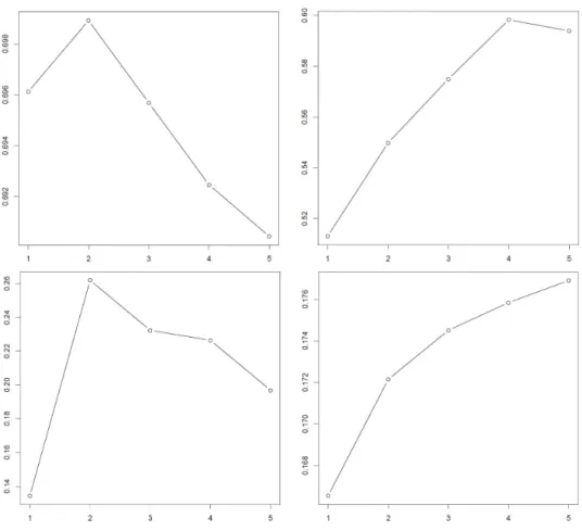
in the k clusters and its expectation under a null reference distribution generated by Monte Carlo sampling. The gap statistic analysis was independently performed for each transformation applied to the data (log-transform, PCA, tSNE, TF-IDF, etc.) as the gap statistics, and hence the optimal number of clusters, are sensitive to these transformations (Figure 2.2).

The gap statistic based estimate was used to directly specify the number of clusters for all methods exceptSeurat, Seurat SNN and graph-based clustering algorithms, which determine the number of clusters internally.

(13)

Figure 2.2: Clockwise from top left: gap statistics for log-transformed, log-transformed PCA, tSNE, and TF-IDF transformed and binarized expression levels of a 7:1 mixture of regulatory t and naive t cells. The x-axis gives the number of clusters K and the y-axis gives the gap statistic in (2.1).

algorithms was lower than the gap statistic estimate additional partitioning steps were performed as described below to enforce a minimum number of clusters.

2.2.1 Existing scRNA-Seq clustering methods

We included in our comparison several commonly used methods. First, we included two methods from the Seurat package [44], one based on K-means and one based on graph clustering. Following the Granatum pipeline [55], we included K-means and hierarchical clustering with Euclidean and Pearson distances based on a 2-dimensional projection of the data using the t-distributed Stochastic Neighbor Embedding (tSNE) transformation [51]. Also from Granatum, we tested K-means using the log2(x+1) transformed data. Using the log2(x+1) transform of the data followed by PCA, we tested a Gaussian Mixture Model (GMM) based algorithm, a K-means algorithm similar to that implemented in the

(14)

CellRanger pipeline distributed by 10x Genomics [18], as well as spherical K-means and hierarchical clustering algorithms, again with both Euclidean and Pearson correlation distances. Finally, similar to the graph-based algorithms implemented in the latest version of the CellRanger pipeline [18], we tested the graph-based Louvain clustering algorithm [4] with Euclidean distance over log2(x+1) transformed data. Details on individual methods can be found in [39].

Details on individual methods are as follows.

Seurat, Seurat SNN

To test Seurat, we followed the guided clustering workflow recommended in the tutorial at [1] by first applying the recommended cell quality filtering based on the number of detected genes, minimum 200 per cell, and percentage of reads from mitochondrial genes. Then, as recommended by Seurat’s authors, we ‘regressed out’ uninteresting sources of variation such as technical noise and batch effects. As suggested in [5], regressing out these effects improves downstream dimensionality reduction and clustering. We then used Seurat’s MeanVarPlot() with its default values to identify genes that are outliers on the ‘mean variability plot’ as recommended by Seurat’s authors. After selecting highly variable genes and performing PCA analysis, we used Seurat’s DOKMeans() function which performs K-means clustering on both genes and cells; we refer to this method as

Seurat in the Results section. We also used the FindClusters() function which uses the

top principal components and identifies clusters of cells by a shared nearest neighbor (SNN) modularity optimization based clustering algorithm that first calculates k-nearest neighbors and constructs the SNN graph, then optimizes the modularity function to determine clusters; this method is referred to as Seurat SNN.

Gaussian Mixture Model based clustering (Log PCA GMM)

We used the mclust R package [17] to perform clustering by fitting a finite Gaussian Mixture Model (GMM) using expectation-maximization. We first performed Principal Component Analysis (PCA) of the log2(x+1) transformed UMI count matrix and ran

(15)

mclust on the top 10 principal components.

K-means clustering variants (Log Kmeans, Log PCA Kmeans, tSNE Kmeans)

K-means clustering [21]

aims to partition n points (cells in our case) intok clusters such that the total intra-cluster variance is minimized. Motivated by the similar intra-clustering option provided in the Granatum pipeline from [55] we included in the comparison a K-means variant (called

Log Kmeans) that takes as input the log2(x+1) transformed UMI counts. We also

fol-lowed an approach similar to that adopted in the CellRanger pipeline distributed by 10x Genomics [18], referred to as Log PCA Kmeans, in which the PCA is run on the log2(x+1) transformed UMI counts and K-means clustering is performed on the first 10 principal components. Finally, and again motivated by the Granatum pipeline from [55], we included a K-means variant run on the 2-dimensional tSNE transformation of the data

(tSNE Kmeans).

Spherical K-means with log transform and PCA (Log PCA sKmeans)

In this method we used the spherical K-means algorithm [22] to cluster the log2(x+1) and PCA transformed data. Instead of Euclidean distance, spherical K-means employs

the cosine dissimilarity,

1−cos(θ) = 1− n P i=1 AiBi r _n P i=1 A2 i r _n P i=1 B2 i (2.2)

based on the angle between two feature vectors A and B, which has been shown to be more robust to large differences in total vector weights. We added this method here as we wanted to compare its performance with the spherical K-means applied to TF-IDF transformed data described in next subsection.

(16)

Hierarchical Clustering variants (Log PCA HC E, Log PCA HC P, tSNE HC E, tSNE HC P)

Agglomerative hierarchical clustering is a “bottom up” approach: each observation starts in its own cluster, and pairs of clusters are iteratively merged based on inter-cluster dis-tances. Ward’s method [52] was used as linkage criterion. We included in the com-parison four variants of hierarchical clustering, in which the algorithm was run us-ing Euclidean and Pearson correlation distances on either the first 10 principal com-ponents of the log2(x+1) UMI counts (methods referred to as Log PCA HC E and

Log PCA HC P, respectively), or on the 2-dimensional tSNE transformation of the data

as in [55] (tSNE HC E and tSNE HC P).

Graph based Louvain clustering algorithm (Log Louvain E)

We also included in our comparison a graph-based Louvain clustering algorithm similar to that provided by the current version of the CellRanger pipeline distributed by 10x Genomics [18]. This method takes as input the log2(x+1) transformed UMI counts and builds a graph by connecting pairs of cells with Euclidean pairwise distance above a certain threshold. For our experiments we scaled the distance values to the range 0 to 1 and set a cutoff of 0.01 to build a rather dense but weighted graph. We then apply the Louvain for modularity optimization [4] as implemented in igraph R [12] package to identify communities (clusters) of cells.

Different from our method, the CellRanger pipeline implements Louvain modularity optimization on a sparse nearest-neighbor graph, where each cell is linked to its k nearest Euclidean neighbors, where k is set to scale logarithmically with the number of cells. CellRanger’s implementation also includes an additional cluster-merging step which con-sists of hierarchical clustering on the cluster-medoids in PCA space followed by merging of sibling clusters with no differentially expressed genes at an FDR of 0.05; such a step was not included in our implementation.

(17)

2.2.2 TF-IDF scoring

TF-IDF, which stands forTerm Frequency times Inverse Document Frequency, is a data transformation and a scoring scheme typically used in text analyses for measuring whether or not and how concentrated into relatively few documents the occurrences of a given word are [29]. Given a collection ofN documents, and letfij be the number of occurrences

of word i in document j. Theterm frequency of word i in document j, denoted by T Fij,

is defined as

T Fij =fij/max

k fkj (2.3)

Here, the term frequency of wordiin documentjis the number of occurrences normalized by dividing it by the maximum number of occurrences of any word in the same docu-ment, sometimes this is done after excluding stop words. The normalization is needed to make it possible to compare term frequencies for documents of different lengths. After normalization, the most frequent word in a document always gets a term frequency value of 1, while other words get fractional values as their respective term frequencies. The

Inverse Document Frequency of wordi is defined as

IDFi = log2(N/ni). (2.4)

where ni denotes the number documents that contain word i among the N documents

in the collection. Finally, the TF-IDF score for word i in document j is defined to be

T Fij ×IDFi. Words with the highest TF-IDF score in a document are often the terms

that best characterize the topic of that document.

To apply TF-IDF scores for scRNA-Seq data we consider the cells to be analogous to documents; in this analogy, genes correspond to words and UMI counts replace word counts. The TF-IDF scores can then be computed from UMI counts using equations (2.3) and (2.4). Similar to document analysis, the genes with highest TF-IDF scores in a cell are expected to provide most information about the cell’s type.

We explored two different approaches of using TF-IDF scores for scRNA-Seq cluster-ing. In first approach TF-IDF scores were used to select a subset of the most informative

(18)

Figure 2.3: Highly variable genes for a 1:1 mixture of b cells and cd14 monocytes. genes that were then used for performing clustering. In the second approach all genes are used for clustering but the gene expression data was first binarized based on a TF-IDF cutoff. Each of these data transformations were combined with a number of clustering algorithms, as detailed in the following two subsections.

2.2.3 scRNA-Seq clustering based on TF-IDF gene selection

We tested two alternatives methods for TF-IDF based gene selection: using the genes with highest TF-IDF average and using the genes with highest variability in TF-IDF values.

In the first method, referred to as Top, we fitted a 2-mixture GMM model to the distribution of TF-IDF gene averages using mclust, and selected the genes assigned to the mixture component with highest mean. In case this resulted in a list of more than 3,000 genes, we retained only the top 3,000 genes when ranking the genes based on the number cells in which they are detected.

(19)

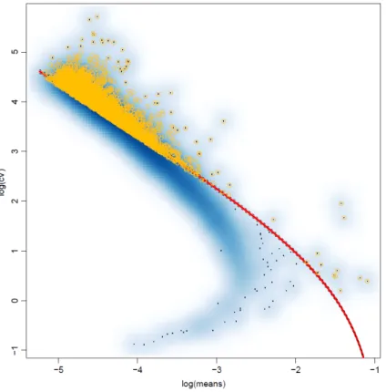
vari-ability by analyzing the relationship between the coefficient of variation (CV) and average expression levels as described in [8]. We first computed for each gene the sample TF-IDF mean and coefficient of variation CV, which is a standardized measure of dispersion. We then fitted a regression line for the observed pairs of mean/CV values (plotted on log-log scale in Figure 2.3). Finally, we computed for each gene the difference between the observed CV and the CV expected for the observed mean based on the regression line, and retained for clustering analysis only the top 30% of the genes ranked by this difference (shown in yellow in Figure 2.3).

After applying the TF-IDF transform to the UMI count matrix and performing gene selection using the above two methods, clustering was performed using one of the following algorithms:

Gaussian Mixture Model based clustering (TF-IDF Top GMM, TF-IDF Var GMM).The

expectation-maximization clustering algorithm implemented in the mclust R pack-age [17] was applied to the TF-IDF scores of genes selected using the Top, respec-tively Var methods.

K-means (TF-IDF Top Kmeans, TF-IDF Var Kmeans). Similarly, we applied K-means

clustering to the TF-IDF scores of genes selected using either Top orVar.

Spherical K-means (TF-IDF Top sKmeans, TF-IDF Var sKmeans). We also used the

spherical K-means algorithm [22] on TF-IDF scores of genes selected using Top, respectively Var.

Hierarchical Clustering (TF-IDF Top HC E, TF-IDF Top HC P, TF-IDF Top HC C,

TF-IDF Var HC E, TF-IDF Var HC P, TF-IDF Var HC C).Finally, we performed

hierarchical clustering with Ward aggregation on the TF-IDF scores of selected genes using Euclidean, Pearson correlation, as well as cosine distance (2.2) – the latter metric was included as it is often employed in conjunction with TF-IDF for text analysis [13].

(20)

Figure 2.4: Left: Distribution of TF-IDF gene averages for a 1:1 mixture of memory and regulatory T cells. Right: Binarization cutoff effect on macro accuracy of TF-IDF Bin HC C method on the same cell mixture.

2.2.4 scRNA-Seq clustering using TF-IDF based binarization

The distribution of mean TF-IDF scores of the genes (plotted for a mix of 1,000 memory and 1,000 regulatory T cells in the left panel of Figure 2.4) typically exhibits a long tail. The genes with very high mean TF-IDF scores are potentially the most informative in identifying the underlying cell types. The final group of TF-IDF based methods uses this intuition by binarizing the gene expression data. We first selected a suitable TF-IDF cutoff and then, for each cell, we set the expression signature of all genes with a TF-IDF above the cutoff to 1, and all remaining signatures to 0. Cells sharing the same type are expected to have highly similar 0/1 expression signature vectors. By setting to 1 only the ‘informative’ genes in each cell we aim to remove unnecessary noise and achieve better clustering accuracy. Although the choice of TF-IDF cutoff can affect the clustering accuracy, as shown in the right side of Figure 2.4) for a sample cell mixture, near maximum accuracy is achieved by using a cutoff value equal to 0.1 × the mean of the per-cell non-zero TF-IDF values. All experimental results presented in the Results section are based on this cutoff.

The resulting binary expression signatures were then clustered using one of the fol-lowing algorithms:

Hierarchical clustering with Euclidean, Pearson, cosine and Jaccard distances

(TF-IDF Bin HC E, TF-(TF-IDF Bin HC P, TF-(TF-IDF Bin HC C, TF-(TF-IDF Bin HC J).

Hi-erarchical clustering with Ward aggregation was applied to the binarized TF-IDF expression signature vectors using Euclidean, Pearson correlation, and cosine

(21)

dis-tances (2.2), respectively, to compare with the previous variations of hierarchical clustering based on the same distances. Additionally, we performed hierarchical clustering with Ward aggregation using the Jaccard distance to measure dissimi-larity between cells. This is defined as 1 - Jaccard simidissimi-larity, where the Jaccard

similarity between two cells is computed as the number of genes with a signature

of 1 in both cells divided by the number of genes with a signatures of 1 in at least one of the cells.

TF-IDF graph-based Greedy clustering with Euclidean, Pearson, cosine and Jaccard distances (TF-IDF Bin Greedy E, TF-IDF Bin Greedy P, TF-IDF Bin Greedy C,

TF-IDF Bin Greedy J).In these methods we begin by building an undirected graph

with cells as the vertices and edges connecting pairs of cells for which the binarized expression signature vectors have Euclidean, Pearson, cosine, or Jaccard distance below a certain cutoff value. For our experiments we set a rather low cutoff of 0.01 to to build a dense graph, but weighted the edges of this graph by the correspond-ing pairwise similarity measures for clustercorrespond-ing by greedy modularity optimization, which was performed using the algorithm introduced in [9] and implemented in the cluster fast greedy() function of the igraph R package [12]. To ensure the ho-mogeneity of resulting clusters and to force a minimum number of clusters when required, all clusters with a silhouette score below a given threshold were subjected to further partitioning. All cells in such a cluster were used to form a new gene ex-pression matrix which was subjected to TF-IDF transformation, binarization, and then clustering via the greedy modularity optimization algorithm. The process was repeated until the minimum number of clusters was achieved, or no cluster had a silhouette score below the given threshold.

TF-IDF graph-based Louvain clustering with Euclidean, Pearson, cosine and Jaccard dis-tances (TF-IDF Bin Louvain E, TF-IDF Bin Louvain P, TF-IDF Bin Louvain C,

TF-IDF Bin Louvain J).Here, the same approach described above for graph-based

Greedy clustering was used in conjunction with the Louvain modularity optimiza-tion algorithm [4] as implemented in the cluster louvain() funcoptimiza-tion of the igraph R

(22)

Figure 2.5: Left: Correlation distances between mean expression levels of 7 immune cell types from [53]. Right: 3D PCA plot of 1000 cells of each type.

package [12].

2.2.5 Experimental setup

Datasets

To assess the accuracy of compared clustering methods we used synthetic mixtures of real scRNA-Seq profiles generated from FACS sorted immune cells using the 10x Genomics platform [53]. We started from the filtered UMI count matrices generated using the CellRanger pipeline and made publicly available at https://support.10xgenomics.com/ single-cell-gene-expression/datasets. Of the available sorted cell populations we excluded those shown to have substantial heterogeneity in [53]. This left us with seven cell types: CD4+/CD25+ Regulatory Cells (regulatory t), CD4+/CD45RO+ Memory Cells (mem-ory t), CD19+ B Cells (b cells), CD14+ Monocytes (cd14 monocytes), CD56+ Natural Killer Cells (cd56 nk), CD8+/CD45RA+ Naive Cytotoxic T Cells(naive cytotoxic), and CD4+/CD45RA+/CD25- Naive T cells (naive t).

The hierarchical clustering dendrogram based on Pearson correlations between mean gene expression levels of the seven cell types along with a 3-dimensional PCA projection of the individual scRNA-Seq profiles are shown in Figure 2.5.

Clearly, B cells, NK cells and monocytes are relatively dissimilar to each other and to the four T cell types, which in turn form two highly similar pairs (memory t and

(23)

naive cytotoxic) and (regulatory t and naive t) and pairs with intermediate dissimilarity like (memory t and naive t) and (regulatory t and naive cytotoxic). Thus, in a first set of experiments, we focused on mixtures of cells generated from six pairs of cell types of varying degrees of dissimilarity.

We chose pairs (b cells and cd14 monocytes) and (b cells and cd56 nk) to represent mixtures of highly dissimilar cell types, pairs (memory t and naive cytotoxic) and (regula-tory t and naive t) to represent mixtures of highly similar cell types, and pairs(memory t and naive t) and (regulatory t and naive cytotoxic) to represent mixtures of cell types with intermediate similarity. To assess clustering accuracy in the presence of different levels of imbalance between the numbers of cells of different types, for each of the six pairs of cell types we generated mixtures in ratios 7:1, 3:1, 1:1, 1:3, and 1:7. For each mixture ratio, we sampled a total of 1,000 cells from the corresponding cell types. Finally, to assess accuracy on a more complex cell population, we generated mixtures comprised of 7,000 cells sampled from all seven cell types in equal proportions.

We also tested the implemented methods on scRNA-Seq data from [46].

Single-cell RNA-Seq libraries were generated using the Smart-seq2 protocol and se-quenced on an Illumina HiSeq 2000.

For this dataset we included all cells without any quality filtering to reflect as close as possible the natural frequency of these cell types in pancreatic islets. As in [26], marker genes with unusually high expression levels (INS for beta cells, GCG for alpha cells, SST for delta cells, PPY for PP/gamma cells, and GHRL for epsilon cells) were removed prior to clustering to eliminate the possibility that they drive the clustering by themselves. A hierarchical clustering dendrogram based on the Pearson correlation between mean gene expression levels of the seven cell types and a 3-dimensional PCA projection of the individual scRNA-Seq profiles are shown in Figure 2.6.

(24)

Figure 2.6: Left: Correlation distances between mean expression levels of 7 pancreatic island cell types from [46]. Right: 3D PCA plot of the 2,045 pancreatic island cells.

Accuracy measures.

For each dataset we computed macro- and micro-accuracy measures [27],[50] defined by:

Micro Accuracy= K X i=1 Ci/ K X i=1 Ni (2.5) Macro Accuracy= 1 K K X i=1 Ci Ni (2.6) where K is the number of classes, Ni is the number of samples in class i, and Ci is the

number of correctly labeled samples in class i. Note that macro- and micro-accuracy are identical for 1:1 mixtures, but may differ significantly for imbalanced datasets, as macro-averaging gives equal weight to the accuracy of each class (average accuracy of all classes’ accuracies), whereas micro-averaging gives equal weight to each cell classification decision (overall accuracy). The ground truth was based on the cell sorting information and annotations from [53] and [46].

For methods that identified more clusters than expected (more than two clusters for the 2-class experiments or more than seven for the 7-class mixtures), we used majority based matching to label clusters with cell types. For example, if a predicted cluster hasx

cells labeled as cell type C1 in the ground truth andy cells labeled as cell type C2, then all cells are assumed to be predicted as cell type C1 for relevant accuracy calculations

(25)

when x > y. This approach ensures that methods that are more sensitive to the existing heterogeneity within the true cell types are not penalized as long as the resulting sub-clusters are “pure”, i.e., all or most cells of that sub-cluster belong to only one of the cell types contributing to the mixture.

All datasets used in this work along with a Shiny application that performs accuracy calculations for user uploaded clustering results are available at http://cnv1.engr.uconn. edu:3838/SCA/.

2.3 Results and discussion

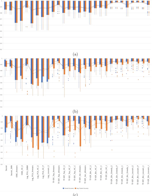
Each of the 36 clustering algorithms described in the Methods section was run on 2-class synthetic mixtures of 1,000 cells sampled in different ratios from six pairs of immune cell types as described in Experimental setup. For each combination of cell types and mixture ratio we repeated each experiment five times and computed the macro- and micro-accuracy using equations (2.5)-(2.6). Box-and-whiskers plots displaying the macro-and micro-accuracies of the compared algorithms, grouped into three categories (existing methods, algorithms using TF-IDF based gene selection, and algorithms using TF-IDF binarization), are shown in Figure 2.7. Each plot shows the median of the corresponding measure as the middle horizontal line, along with mean values as the middle points connected by lines across methods. The whiskers indicate the extreme non-outlier data points of the upper and lower quartiles. If present, outliers, i.e., data points that lie more than 1.5 interquartile ranges below the first quartile or above the third quartile, are indicated as single points on the plot.

Overall, algorithms using TF-IDF binarization have consistently high accuracy in all 2-class experiments, with existing methods and algorithms using TF-IDF based gene selection showing a higher degree of variability in accuracy across datasets. For remain-ing results we eliminated 8 methods that show consistently lower clusterremain-ing accuracy in the 2-class experiments. Specifically, from the existing methods group we removed from further analysis tSNE HC P, Log Kmeans, and Log PCA sKmeans, all of which have

(26)

(a)

(b)

(c)

Figure 2.7: Micro and macro accuracy on 2-class synthetic mixtures of immune cells with ratios 1:1, 1:3/3:1, and 1:7/7:1 for (a) existing methods, (b) algorithms using TF-IDF based gene selection, and (c) algorithms using TF-IDF binarization.

(27)

both macro and micro-accuracy averages below 0.8. From the group of methods using TF-IDF based gene selection we removed the two GMM methods (TF-IDF Top GMM and TF-IDF Var GMM), which clearly performed much worse than the rest. We also re-moved the three hierarchical clustering methods using genes with highly variable TF-IDF scores (TF-IDF Var HC E, TF-IDF Var HC P, TF-IDF Var HC C) since their accuracy is worse than the corresponding methods that use the genes with top average TF-IDF score. All twelve algorithms using TF-IDF binarization were retained for further in-depth comparisons.

The macro- and micro-accuracies of the 28 remaining algorithms on 2-class synthetic mixtures with varying mixture ratios and varying difficulties and more discussion of these results can also be found in [6] and [39].

Box-and-whiskers plots displaying the macro- and micro-accuracies of the 28 remain-ing algorithms on 2-class synthetic mixtures with varyremain-ing mixture ratios are shown in Figure 2.8. Among existing methods, the Log PCA GMM EM-based algorithm and Seurat SNN have highest average macro and micro-accuracies, with Log PCA GMM having an edge in average accuracies on the more balanced 1:1 and 1:3/3:1 mixtures, and Seurat SNN yielding slightly better macro-accuracy for the more imbalanced 1:7/7:1 mixtures. However, several TF-IDF based clustering methods achieve higher overall av-erage macro- and micro-accuracies for all mixture ratios, with TF-IDF Bin Louvain C, TF-IDF Bin Louvain P and TF-IDF Top sKmeans scoring the highest. For imbalanced mixtures, the micro-accuracy is usually lower than but closely tracks macro-accuracy, generally preserving the relative performance of the compared methods.

Plots displaying the macro- and micro-accuracies of the 28 methods grouped by the level of similarity of the two cell types in the mixtures are given in Figure 2.9.

As expected, all methods have very high clustering accuracy on mixtures of highly dissimilar cell types. The accuracy is generally lower on mixtures of cell types with intermediate similarity, and lower still on mixtures of highly similar cell types. Algo-rithms based on TF-IDF binarization perform among the best on all types of mixtures, with TF-IDF Bin Louvain C and TF-IDF Bin Louvain P showing most consistent

(28)

per-(a)

(b)

(c)

Figure 2.8: Micro and macro accuracies on 2-class synthetic mixtures with ratios 1:1 (a), 1:3/3:1 (b), and 1:7/7:1 (c).

(29)

(a)

(b)

(c)

Figure 2.9: Micro- and macro-accuracies for synthetic mixtures with ratios 1:1, 1:3/3:1, and 1:7/7:1 simulated from (a) highly dissimilar cell type pairs (cd14 monocytes,b cells) and (cd56 nk,b cells), (b) intermediate similarity cell type pairs (regulatory t,naive cytotoxic) and (memory t,naive t), and (c) highly similar cell type pairs (regulatory t,naive t) and (memory t,naive cytotoxic).

(30)

Figure 2.10: Accuracy for equal-proportion 7-way mixtures of immune cell types (1000 cells each).

formance. The TF-IDF Top sKmeans algorithm is best-performing within the group of algorithms using TF-IDF based gene selection, with only slightly lower performance than TF-IDF Bin Louvain C and TF-IDF Bin Louvain P on mixtures of highly similar pairs. To assess the effect of increased population complexity on accuracy, we also ran the 28 methods on equal-proportion mixtures consisting of all seven immune cell types from [53].

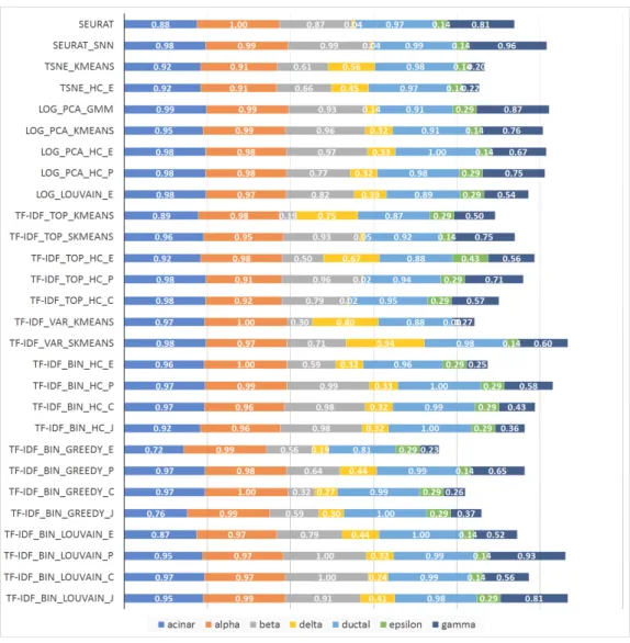
The accuracies achieved for each cell type are shown in Figure 2.10. Since the cell types were mixed in equal proportions in this experiment, the macro- and micro-accuracy of each method are equal to the average accuracy over all cell types, and hence proportional to the total length of the horizontal bars in the figure. These mixtures contain both highly similar and highly dissimilar cell types, and several methods end up assigning

(31)

Figure 2.11: Accuracy for pancreatic cells based on the RPKM values.

highly similar cell types to a single cluster, resulting in significantly reduced accuracy for some of the cell types. TF-IDF Bin Louvain C is least affected by such miss-assignments, achieving the best overall accuracy.

Figure 2.11 show the accuracy per cell type for experiments on the scRNA-Seq dataset from [46], consisting of 2,045 pancreatic islet cells annotated with one of seven cell types. Since cell type abundances in this dataset reflect their natural frequency in pancreatic islets, the total length of the horizontal bars in the figure is proportional with the macro-accuracy (but not necessarily micro-macro-accuracy) of each method. Two sets of results are presented, one based on raw counts and one based on RPKM values in [46]. The relative performance of the compared methods on this dataset is quite different from that on the 7-way mixture in Figure 2.10, underscoring the fact that the performance of clustering

(32)

algorithms is highly dependent on specific aspects of each dataset. The relative perfor-mance is also dependent on the metric used, with raw counts yielding a quite different ranking of methods compared to RPKMs.

Tables 2.1 and 2.2 from [39] summarizes the results of all experiments by giving the average rank (among the 28 selected methods) achieved on each dataset based on macro-, respectively micro-accuracy, along with overall rank averages that give equal weight to each dataset. TF-IDF Bin Louvain C has the lowest overall average rank with respect to both macro- and micro-accuracy. The next three best performers with respect to overall average rank for both macro- and micro-accuracy are all based on the TF-IDF transform as well (in order, IDF Bin Louvain P, IDF Bin Louvain E, and TF-IDF Top sKmeans), with TF-TF-IDF Bin Greedy P coming fifth in macro-accuracy overall average rank (Log PCA GMM takes fifth place for micro-accuracy average rank).

2.4 Conclusion

In this work we compared twenty eight methods for clustering scRNA-Seq data: nine commonly used existing approaches and nineteen methods based on the use of TF-IDF scores similar to those used in the text analysis field. Empirical experiments on a variety of cell types and ratio mixtures suggest that TF-IDF based methods achieve consistently high accuracy, even on complex mixtures of highly similar cell types.

A limitation of the TF-IDF Bin HC methods’ group is the quadratic time required for distance calculations used in hierarchical clustering methods, which becomes a per-formance bottleneck for datasets with millions of single cells. We are also exploring TF-IDF based feature selection further in our future work, an interpretable way of using the Genes’ average TF-IDF score was used to visualize the data and clustering results as described in Part III of this document.

(33)

Table 2.1: Average ranks based on micro-accuracy. The lowest five average ranks (in-cluding ties) for each dataset are typeset in bold, and the best overall average rank is shown in red.

Methods M Nc R N M N R Nc B Nk B Mc 7-class Pancreas Avg.

Seurat 14.6 19.0 25.0 25.6 1.0 25.6 28.0 4.0 17.9

Seurat SNN 6.8 13.8 21.0 18.4 1.0 25.6 26.6 1.0 14.3

tSNE Kmeans 26.0 27.0 14.6 18.6 22.6 27.8 11.4 19.5 20.9

tSNE HC E 25.0 25.4 12.6 18.0 6.0 11.2 10.0 20.0 16.0

Log PCA GMM 20.8 10.6 2.4 12.8 1.0 1.0 4.4 14.5 8.4

Log PCA Kmeans 24.4 24.4 26.4 26.8 1.0 1.0 7.6 14.0 15.7

Log PCA HC E 23.8 22.8 22.6 23.8 1.0 1.0 4.6 14.0 14.2

Log PCA HC P 27.0 25.2 25.4 26.0 16.4 6.0 2.4 18.5 18.4

Log Louvain E 26.2 27.2 25.8 21.0 15.4 6.2 10.4 14.0 18.3

TF-IDF Top Kmeans 6.0 16.8 15.8 17.0 1.0 1.0 9.2 21.0 11.0

TF-IDF Top sKmeans 2.0 7.4 7.0 2.4 1.0 1.0 8.4 9.5 4.8

TF-IDF Top HC E 20.4 21.0 24.4 23.4 1.0 1.0 19.8 18.5 16.2

TF-IDF Top HC P 14.8 15.8 19.2 16.0 1.0 1.0 16.4 12.0 12.0

TF-IDF Top HC C 14.6 17.0 17.4 15.4 1.0 1.0 18.0 14.5 12.4

TF-IDF Var Kmeans 7.2 10.6 19.0 24.2 10.0 1.0 25.8 21.5 15.0

TF-IDF Var sKmeans 11.0 15.2 19.4 18.2 1.0 1.0 20.2 4.5 11.3

TF-IDF Bin HC E 21.0 21.4 17.4 14.6 1.0 1.0 17.0 19.5 14.1

TF-IDF Bin HC P 13.6 9.4 8.4 9.2 1.0 1.0 8.0 6.0 7.1

TF-IDF Bin HC C 14.0 10.8 11.4 9.2 1.0 1.0 10.6 8.5 8.3

TF-IDF Bin HC J 17.4 13.2 13.4 9.8 1.0 1.0 12.8 14.0 10.3

TF-IDF Bin Greedy E 11.6 7.4 7.2 8.8 18.8 5.8 23.8 27.0 13.8

TF-IDF Bin Greedy P 4.6 4.6 5.2 2.4 5.0 1.0 19.0 12.0 6.7

TF-IDF Bin Greedy C 5.2 5.2 7.8 2.8 23.2 1.0 19.4 28.0 11.6

TF-IDF Bin Greedy J 16.2 9.4 10.6 6.4 5.8 1.0 18.0 24.5 11.5

TF-IDF Bin Louvain E 5.8 2.0 3.2 2.4 5.0 1.0 4.2 13.0 4.6

TF-IDF Bin Louvain P 1.0 1.4 1.8 1.4 1.0 1.0 14.2 4.0 3.2

TF-IDF Bin Louvain C 1.2 2.0 1.6 1.0 1.0 1.0 1.2 11.5 2.6

TF-IDF Bin Louvain J 9.6 6.2 6.0 2.8 18.4 1.0 11.8 7.0 7.9

2.5 Availability of data and materials

Datasets used in this work are available for download from http://cnv1.engr.uconn.edu: 3838/SCA/. The application also provides accuracy calculations for user uploaded clus-tering results. Also, the proposed TF-IDF analysis approach is implemented in the web-based scRNA-Seq data analysis tool available at http://sc1.engr.uconn.edu. This tool further implements the work-flow analysis that is presented in the last chapter of this work.

(34)

Table 2.2: Average ranks based on macro-accuracy. The lowest five average ranks (in-cluding ties) for each dataset are typeset in bold, and the best overall average rank is shown in red.

Methods M Nc R N M N R Nc B Nk B Mc 7-class Pancreas Avg.

Seurat 8.2 8.0 18.8 24.2 1.0 26.4 27.2 10.0 15.5

Seurat SNN 9.0 9.2 18.0 19.4 1.0 27.0 27.0 3.5 14.3

tSNE Kmeans 24.2 24.0 9.0 14.8 22.4 26.6 11.6 18.5 18.9

tSNE HC E 24.4 24.8 9.4 18.2 6.2 10.4 9.2 20.0 15.3

Log PCA GMM 20.4 6.4 3.0 4.8 1.0 1.0 4.4 14.0 6.9

Log PCA Kmeans 27.2 27.4 26.6 26.8 1.0 1.0 7.6 16.0 16.7

Log PCA HC E 27.2 24.8 22.0 24.6 1.0 1.0 4.8 13.5 14.9

Log PCA HC P 25.8 23.8 17.8 20.6 16.2 5.6 2.4 18.0 16.3

Log Louvain E 23.0 25.6 20.8 14.2 15.0 5.8 10.6 14.5 16.2

TF-IDF Top Kmeans 9.6 13.4 18.6 13.6 1.0 1.0 9.6 18.5 10.7

TF-IDF Top sKmeans 4.2 9.4 8.0 6.2 1.0 1.0 8.6 12.5 6.4

TF-IDF Top HC E 21.4 19.2 25.6 23.6 1.0 1.0 17.4 13.0 15.3

TF-IDF Top HC P 17.6 17.4 20.4 20.6 1.0 1.0 18.2 11.5 13.5

TF-IDF Top HC C 17.0 16.2 20.6 21.2 1.0 1.0 20.4 12.5 13.7

TF-IDF Var Kmeans 12.0 21.0 27.4 27.6 19.6 19.0 26.4 24.0 22.1

TF-IDF Var sKmeans 11.8 18.0 23.4 18.6 1.0 1.0 21.6 2.5 12.2

TF-IDF Bin HC E 20.2 22.2 19.8 16.6 1.0 1.0 19.2 21.0 15.1

TF-IDF Bin HC P 15.4 13.2 12.0 12.2 1.0 1.0 8.4 4.5 8.5

TF-IDF Bin HC C 15.8 15.2 13.2 11.4 1.0 1.0 10.8 5.5 9.2

TF-IDF Bin HC J 17.8 15.8 14.0 12.8 1.0 1.0 13.0 12.0 10.9

TF-IDF Bin Greedy E 7.0 5.2 5.4 4.8 20.0 1.0 23.0 27.0 11.7

TF-IDF Bin Greedy P 3.8 4.2 4.4 2.2 1.0 9.8 19.2 11.0 7.0

TF-IDF Bin Greedy C 4.8 5.0 5.6 3.2 1.0 9.8 19.4 26.5 9.4

TF-IDF Bin Greedy J 13.8 10.2 11.0 6.2 10.2 1.0 16.2 22.0 11.3

TF-IDF Bin Louvain E 4.4 2.6 3.4 6.4 1.0 1.0 4.2 16.0 4.9

TF-IDF Bin Louvain P 1.2 3.4 2.4 2.4 10.0 1.0 11.2 4.0 4.5

TF-IDF Bin Louvain C 1.0 3.0 1.8 2.4 5.2 1.0 1.2 11.5 3.4

(35)

Chapter 3 LSImpute: Locality Sensitive

Imputation for Single Cell RNA-Seq

Data

3.1 Introduction

Emerging single cell RNA sequencing (scRNA-Seq) technologies enable the analysis of transcriptional profiles at single cell resolution, bringing new insights into tissue hetero-geneity, cell differentiation, cell type identification and many other applications. The scRNA-Seq technologies, however, suffer from several sources of significant technical and biological noise, that need to be addressed differently than in bulk RNA-Seq.

One of the most notable challenges is the so called ‘drop-out’ effect. Whether occurring because of inefficient mRNA capture, or naturally due to low number of RNA transcripts and the stochastic nature of gene expression, the result is capturing only a fraction of the transcriptome of each cell and hence data that has a high degree of sparsity. The drop-outs typically do not affect the highly expressed genes but may affect biologically interesting genes expressed at low levels such as transcription factors. Combining cells as a measure to compensate for the drop-out effects could be defeating the purpose of performing single cell RNA-Seq. In this work we take advantage of the random nature of

(36)

drop-outs and develop imputation methods for scRNA-Seq. In next section we briefly discuss some existing scRNA-Seq imputation methods and propose a novel iterative imputation approach based on efficiently computing highly similar cells. We then present the results of a comprehensive assessment of the existing and proposed methods on real scRNA-Seq datasets with varying sequencing depth.

3.2 Methods

3.2.1 Existing single cell RNA-Seq imputation methods

Several methods were studied and tested: DrImpute [25], scImpute [31], and KNNImpute [49]. The existing methods are discussed in more details in our paper [38].

3.2.2 Proposed method: locality sensitive imputation

(LSIm-pute)

We propose a novel algorithm that uses similarity between cells to infer missing values in an iterative approach. The algorithm summary is as follows:

Step 1. Given a set S of n cells (represented by their scRNA-Seq gene expression profiles), start by selecting pairs of cells with highest similarity level until at least mmin

distinct cells (mmin = 6 in our implementation) are selected or the highest pair similarity

drops below a given threshold. This process guarantees that each selected cell has highest pairwise similarity level to at least one other selected cell.1

Step 2. Cluster them cells selected in Step 1 using a suitable clustering algorithm (our implementation uses spherical K-means withk =√m). The clusters formed in this step are expected to be “tight”, with each selected cell having high similarity to the other cells in its cluster.

1_{Note that, unlike KNN, which uses similarity between genes, LSImpute uses similarity between cells.}

Also, the number of nearest cells used for imputation is not fixed but depends on the minimum similarity threshold.

(37)

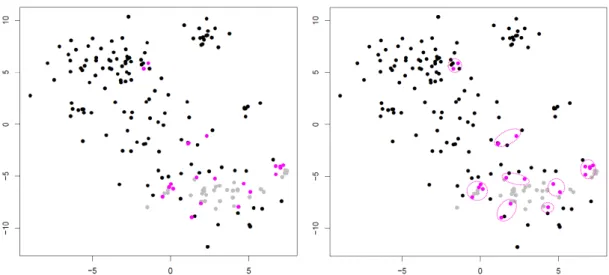
Figure 3.1: Illustration of Steps 1 (left) and 2 (right) of LSImpute. Gray dots repre-sent already processed cells and collapsed centroids from previous iterations. Pink dots represent cells in pairs with highest similarity level which are selected for clustering.

Step 3. For each of the clusters identified in step 2, replace zero values for each gene

j with values imputed based on the expression levels of gene j in all the cells within the cluster.

Step 4. The selected cells now have imputed values and the clusters they form are col-lapsed into their respective centroids. The centroids are pooled together with unselected cells to form a new set S, and the process is repeated starting again at Step 1.

Note that, naturally, in Step 3 expression levels are imputed only for original cells and not for centroids but centroid expression levels are used in the imputation process if they are selected in Step 1. The expression levels used to replace the zero expression values can be inferred via different models. In Section 3.3 we give results for two simple approaches, namely using the mean, respectively the median of all expression values for gene j in cells belonging to the cluster (these variants are referred to as LSImputeMean, respectively LSImputeMed in Section 3.3). Using the median of both zero and non-zero values first, decides implicitly whether a non-zero is a drop-out event or a true biological effect, and prevents large but isolated expression values from driving imputation of nearby zeros, while collapsing into centroids in each iteration limits the propagation of potential imputation errors. Figure 3.1 illustrates the first two steps of the algorithm.

(38)

● ● ● ● ● ● ● ● ● ● ● ● ● ● ● ● ● ● ● ● ● ● ● ●● ● ● ●● ● ● ● ● ● ● ● ● ● ● ● ● ● ● ● ● ● ●● ● ● ● ● ● ● ●●●● ● ● ● ●● ● ● ● ● ● ● ● ● ● ● ● ●● ● ● ● ●● ● ● ● ● ● ● ● ● ● ● ● ● ● ● ● ● ● ● ● ● ● ● ● ●● ● ● ● ● ● ● ● ● ● ● ● ● ● ● ● ● ● ● ● ● ● ● ● ● ● ● ● ● ● ●●● ● ● ● ● ●● ● ● ●● ● ● ● ● ● ● ● ● ● ● ● ● ● ● ● ● ● ● ● ● ● ● ● ● ●●● ● ● ● ● ● ● ● ● ● ●●●●●● ● ● ● ● ● ● ● −8 −6 −4 −2 0 2 4 6 −10 −5 0 5 10 tSNE−1 tSNE−2 ● ● ● ● ● ● ● ● ● ● ● ● ● ● ● ● ● ● ● ● ● ● ● ● ● ●● ● ● ●● ● ● ● ● ● ● ● ● ● ● ● ● ● ● ● ● ● ●● ● ● ● ● ● ● ●●●● ● ● ● ●● ● ● ● ● ● ● ● ● ● ● ● ●● ● ● ● ●● ● ● ● ● ● ● ● ● ● ● ● ● ● ● ● ● ● ● ● ● ● ● ● ●● ● ● ● ● ● ● ● ● ● ● ● ● ● ● ● ● ● ● ● ● ● ● ● ● ● ● ● ● ● ●●● ● ● ● ● ●● ● ● ●● ● ● ● ● ● ● ● ● ● ● ● ● ● ● ● ● ● ● ● ● ● ● ● ● ●●● ● ● ● ● ● ● ● ● ● ●●●●●● ● ● ● ● ● ● ● ● ● ● ● ● ● CellTypeIDs C1 C2 C3 C4 C5 C6 C7 C8

Figure 3.2: Heatmap of log-transformed TPM values of marker genes identified for DRG neurons in [30] (left) and t-SNE plot showing the 8 clusters from [30] (right).

of remaining cells and centroids starts at n and decreases by at least one in each itera-tion. In practice the number of iterations is much smaller. Our current implementation has two options for finding the pairs of cells with highest similarity level in Step 1. The first option is to use Cosine similarity of [22]. Alternatively, this could be done in O(n) time using Jaccard similarity and Locality Sensitive Hashing [29]. Both similarity metrics are available in the Shiny app available at http://cnv1.engr.uconn.edu:3838/LSImpute/, where the user can also adjust the minimum similarity threshold used in Step 1. It is recommended however to use a high similarity threshold, which will restrict the imputa-tion to only highly similar cells as a way of being conservative with imputaimputa-tion to avoid the risk of over-imputation. A low similarity threshold can lead to imputing more values and can be used when the dataset is of particularly low depths. All results presented in Section 3.3 use Cosine similarity and a minimum similarity threshold of 0.85 for all sets regardless of depth to avoid over-fitting. Using Jaccard similarity based on the R package LSHR [47] resulted in similar imputation levels as the Cosine similarity based implementation.

3.2.3 Experimental setup

Datasets. To assess the performance of the compared imputation methods, we used multiple evaluation metrics on datasets consisting of real scRNA-Seq reads down-sampled to simulate varying sequencing depths per cell. Specifically, we used ultra-deep

(39)

scRNA-Seq data generated for 209 somatosensory neurons isolated from the mouse dorsal root ganglion (DRG) and described in [30]. An average of 31.5M 2×100 read pairs were sequenced for each cell, leading to the detection of an average of 10,950±1,218 genes per cell. To simulate varying levels of drop-out effects we down-sampled the full dataset to 50K, 100K, 200K, 300K, 400K, 500K, 1M, 5M , 10M, respectively 20M read pairs per cell. At each sequencing depthtranscript per million (TPM) gene expression values were estimated for each neuron using the IsoEM2 package [34]. As ground truth we used TPM values determined by running IsoEM2 on the full set of reads. For clustering accuracy evaluation, we used as ground truth the cluster assignment from [30], focusing on the 8 cell populations identified using scRNA-Seq data and not its refinement based on neuron sizes (see Figure 3.2). The C1-C8 clusters we use in this work correspond to the following cell populations identified by their most prominent marker genes as indicated by [30] : C1: Gal; C2: Nppb; C3:Th; C4: Mrgpra3 & Mrgprb4; C5:Mrgprd-high; C6:Mrgprd-low & S100b-high; C7: S100b-low; C8: Ntrk2 & S100b-high.

Evaluation metrics. We used the following metrics to evaluate the imputation meth-ods’ performance at different sequencing depths:

• Detection fraction accuracy. A common application of single cell analyses is to estimate the percentage of cells expressing a given marker gene, for instanceCD4+ orCD8+ tumor infiltrating lymphocytes [15]. A gene is considered to be detected in a cell if the (imputed or ground truth) TPM is positive. For each imputation method, the detection fraction is defined as the number of cells in which the cell is detected divided by the total number of cells. This was compared to the ‘true’ detection ratio, defined based on ground truth TPM values.

• Median percent error (MPE).As defined in [41], theMedian Percentage Error

(MPE) is the median of the set of relative errors for the gene metric examined, in

this case the detection fraction. If a gene has predicted detection fraction y and a ground truth detection fraction ofx, the gene’s relative error is defined as |y−_xx|. For each sequencing depth we computed MPE relative to all genes as well as subsets

(40)

of genes corresponding to the four quartiles defined by gene averages of non-zero ground truth TPM values over all cells (ranges of mean non-zero TPM values for the four quantiles were [0,2.3] (2.3,6.744], (6.744,24.517], and (24.517,18576.98], respectively. Full error curves plotting the percentage of genes with relative error above varying thresholds were also used for a more detailed comparison of imputa-tion methods.

• Gene detection accuracy. This metric views gene detection as a binary classifica-tion problem. For each imputaclassifica-tion method, true positives (TP) are the (gene,cell) pairs for which both imputed and ground truth TPM values are positive, while

true negatives (TN) are (gene,cell) pairs for which both TPM values are zero. The

accuracy is computed as the number of true predictions (T P +T N) divided by the product between the number of genes and the number of cells.

• Clustering micro-accuracy. For each sequencing depth and imputation method we clustered imputed TPM values using several clustering algorithms and assessed the effect of imputation on clustering accuracy using the micro-accuracy measure [27, 50] defined by PK

i=1Ci/

PK

i=1Ni, where K is the number of classes, Ni is the size of class i, and Ci is the number of correctly labeled samples in class i relative

to the ground truth from [30].

3.3 Results and discussion

To assess imputation accuracy on datasets with varying amounts of drop-outs we sub-sampled the ultra-deep DRG scRNA-Seq data to simulate sequencing depths between 50K and 20M read pairs per cell. For each sequencing depth the metrics described in Section 3.2.3 were computed for three previous methods (DrImpute, scImpute and KNNImpute), the two variants of our locality sensitive imputation method described in Section 3.2.2 (LSImputeMean and LSImputeMed), and, as a reference, for the ‘Raw Data’ consisting of TPM values without any imputation.

(41)

Figure 3.3: True vs. imputed detection fractions (left to right: 100K, 1M, 10M read pairs per cell; top to bottom: Raw Data, DrImpute, scImpute, KNNImpute, LSImputeMed,

(42)

Detection fraction accuracy. Figure 3.3 plots the true detection fraction (x-axis) against the detection fraction in the raw data, respectively after imputation with each of the five compared methods (y-axis) at three selected sequencing depths (100K, 1M, respectively 10M read pairs per cell . Each dot in the scatter plots represents one gene. Dot color shades are based on the four quartiles as defined above. For an ideal imputation method all dots would lie on the main diagonal, which represents perfect agreement between predicted and true detection fractions. Dots below the diagonal correspond to genes for which the detection fraction is under-estimated, while dots above the diagonal correspond to genes for which the detection fraction is over-estimated. Drop-outs in the raw data yield severe under-estimation of the detection fraction for most genes at sequencing depths of 100K and 1M read pairs per cell, but at 10M read pairs per cell detection fractions computed based on raw data are very close to the true fractions for nearly all genes. Existing methods over-impute detection fractions for most genes, even at low sequencing depths. At 100K read pairs per cell LSImputeMed under-estimates detection fractions, improving very little over raw values, while LSImputeMean gives most accurate detection fractions. At higher sequencing depths LSImputeMean begins over-imputing, while LSImputeMed yields most accurate detection fractions at 1M read pairs per cell and only slightly over-imputes at 10M read pairs per cell.

Detection fraction error curves and MPE comparison. While dot-plots in Figure 3.3 give a useful qualitative comparison of detection fraction accuracy of different meth-ods, for a more quantitative comparison of detection fraction accuracy Figure 3.4 gives the so called error curve of each method. The error curve plots, for every threshold x

between 0 and 1, the percentage of genes with a relative error above x. The error curves in Figure 3.4 confirm that LSImputeMean has highest detection fraction accuracy of the compared methods at a sequencing depth of 100K read pairs per cell, while LSImputeMed significantly outperforms the other methods at 1M read pairs per cell and matches raw data accuracy at 10M read pairs per cell. The relative performance of the methods can be even more concisely captured by their MPE values, which are the abscissae of the points where the horizontal line with an ordinate of 0.5 crosses the corresponding error

(43)

(a) (b) (c)

Figure 3.4: Error curves for (a) 100K, (b) 1M, respectively (c) 10M read pairs per cell. The abscissa of dashed vertical lines correspond to MPE of raw data.

curves. The surface plots in Figure 3.5 display MPE values (y-axis, on a logarithmic scale) as a function of both sequencing depth (x-axis) and mean non-zero expression quartile (z-axis). The only imputation methods that do not result in MPE values over 100%, depicted in red in the surface plot, are LSImputeMed and LSImputeMean. At all sequencing depths and for all assessed imputation methods genes in the lowest quartile (Q1) have very high MPE, suggesting that detection fractions based on imputed values should not be used for these genes.

Gene detection accuracy and relation to MPE. Table 3.1 shows the gene detection accuracy achieved by the compared imputation methods, with the highest accuracy at each sequencing depth typeset in bold. We assessed gene detection accuracy both based on fractional ground truth and imputed TPM values, as well as after rounding both to the nearest integer, which is equivalent to using a TPM of 0.5 as the detection threshold.

(44)

(a) (b)

(c) (d)

(e) (f)

Figure 3.5: Surface plots indicating Median Percent Error values in log scale (y-axis) for each depth (x-axis) in each quantile (z-axis) for each method: (a) Raw data, (b) DrImpute, (c) scImpute, (d) KNNImpute, (e) LSImputeMed, and (f) LSImputeMean For the results without rounding, DrImpute has the highest gene detection accuracy at 50K and 100K read pairs per cell. LSImputeMean has highest gene detection accuracy for 200K read pairs per cell, while LSImputeMed outperforms the other methods for 300K-1M read pairs per cell. Raw data (no imputation) gives best gene detection accuracy at 5M read pairs per cell and higher depths. For the rounded datasets, DrImpute also has the highest gene detection accuracy at 50K and 100K read pairs per cell, while LSImputeMed outperforms the other methods for 200K-500K read pairs per cell. For sequencing depth of 1M read pairs per cell and higher the raw data gives best detection accuracy followed by LSImpute methods.

At very low sequencing depth it is possible for some methods to impute values that are not detected in the ground truth. This could lead to good performance in detection

(45)

Table 3.1: Gene detection accuracy

Data Not Rounded Rounded

Raw Dr. sc. KNN. LSMd LSMn Raw Dr. sc. KNN. LSMd LSMn 50K 0.676 0.822 0.700 0.799 0.687 0.693 0.752 0.866 0.748 0.700 0.762 0.765 100K 0.740 0.810 0.778 0.713 0.772 0.797 0.816 0.876 0.720 0.712 0.841 0.850 200K 0.800 0.778 0.754 0.726 0.836 0.839 0.872 0.878 0.689 0.722 0.892 0.884 300K 0.829 0.772 0.740 0.732 0.864 0.861 0.899 0.880 0.673 0.726 0.909 0.892 400K 0.847 0.762 0.731 0.736 0.872 0.868 0.915 0.882 0.663 0.730 0.918 0.895 500K 0.859 0.759 0.725 0.738 0.878 0.878 0.927 0.883 0.655 0.732 0.928 0.909 1M 0.891 0.737 0.703 0.747 0.899 0.896 0.952 0.882 0.634 0.738 0.947 0.937 5M 0.918 0.705 0.661 0.762 0.902 0.910 0.980 0.894 0.621 0.772 0.940 0.960 10M 0.920 0.768 0.692 0.648 0.896 0.887 0.987 0.907 0.627 0.800 0.947 0.939 20M 0.921 0.690 0.635 0.774 0.892 0.901 0.994 0.921 0.634 0.825 0.959 0.970

fraction accuracy despite low performance in gene detection accuracy. Furthermore, although one would expect all accuracy measures to improve with increased sequencing depth, this may not necessarily be the case for methods that over-impute.

3.4 Conclusion

Although imputation can be a useful step in scRNA-Seq analysis pipelines, it can become a two-edged sword if expression values are over-imputed. In this work we evaluated the performance of several existing imputation R packages and presented a novel approach for imputation. LSImpute, especially the variant based on median imputation, tends to impute more conservatively than existing methods resulting in improved performance based on a variety of metrics. Overall, LSImpute is more likely to reduce drop-out effects and reduce sparsity of the data without introducing false expression patterns or over-imputation. Cosine and Jaccard similarity based implementations of LSImpute are available as a Shiny app at http://cnv1.engr.uconn.edu:3838/LSImpute/.

(46)

Chapter 4 Cell Cycle Stage and Order

Inference from Single Cell

Transcriptome Data

4.1 Background

The variation in gene expression profiles of single cells that are captured in different phases of the cell cycle can interfere with the functional analysis of the transcriptomic data. In particular, it is important to differentiate between cell type and cell cycle effects when analyzing single cell RNA-Seq data. A first challenge in the computational analysis of the cell cycle effect in single cell transcriptomics is to differentiate between cells that are actively proliferating vs. those that are quiescent, i.e., cells that do not actively divide but retain the ability to re-enter a proliferative state. A second computational challenge is to correctly label individual cells or cell clusters according to their phase in the cell cycle. The main cell cycle phases are G1 (where metabolic changes prepare the cell for division), S (where DNA synthesis replicates the genetic material), G2 (where molecular components needed for mitosis and cytokinesis are assembled), and M (where a nuclear division followed by cytokinesis occurs), although transition phases G1/S and G2/M are also sometimes identified [11]. Such cell labels coupled with existing biological

(47)

knowledge of genes associated with each of the cell cycle phases can assist functional analysis of single cell transcriptional profiles and interpretation of scRNA-Seq clusters. Finally, another computational challenge is to order individual cells according to where they are in the cell cycle. Below we review three existing methods for cell cycle analysis, each trying to address a different challenge:

4.1.1 ccRemover

The ccRemover tool [3] attempts to remove the cell-cycle effect from the single cell tran-scriptional profiles by identifying the principal components that, based on their loadings, capture mostly cell cycle effects. Subtracting the contribution of these components to a low dimensional principal component analysis (PCA) projection of the scRNA-Seq data attempts to enhance the cell type effects on gene expression. We performed an initial test to determine the effectiveness of removing cell cycle effect on a dataset consisting of a 50%:50% mixture of Jurkat and 293T single cells, profiled using the 10x Genomics doplet-based scRNA-Seq platform [18]. This dataset is comprised of cells of two very different types (T lymphocyte and human embryonic kidney cells, respectively) that are well separated according to the original scRNA-Seq profiles (see the 3D tSNE visualiza-tion in Figure 4.10a). However, after transforming the data using ccRemover the two cell lines were indistinguishable (Figure 4.10b), we hence did not include ccRemover method in further method comparisons in this work. Figure 4.10 shows the 3D t-SNE plots of Jurkat-239T data before and after applying ccRemover method. As in [54] we inferred the cluster/library labels based on the expression of cell type-specific markers, the blue cluster corresponds to Jurkat cells (preferentially expressing CD3D), and red corresponds to 293T cells (preferentially expressing XIST, as 293T is a female cell line, and Jurkat is a male cell line). Supplementary Figure 4.11 shows the clustering of cells. We used TF-IDF based Hierarchical Clustering method from [39] and the heat map features the top 50 genes with highest average TF-IDF scores. Both markers, CD3D and XIST that are used in [54] to identify the cell lines in the mixture are selected amongst the list of genes with highest TF-IDF scores.

Computational Methods for the Analysis of Single-Cell RNA-Seq Data

University of Connecticut

OpenCommons@UConn

Computational Methods for the Analysis of

Single-Cell RNA-Seq Data

Marmar Moussa

Computational Methods for the Analysis of

Single-Cell RNA-Seq Data

Computational Methods for the Analysis of

Single-Cell RNA-Seq Data

Contents

Chapter 1

Introduction

Chapter 2

TF-IDF-based Clustering Methods

for Single Cell RNA-Seq Data

2.1

Introduction

2.2

Methods

2.2.1

Existing scRNA-Seq clustering methods

2.2.2

TF-IDF scoring

2.2.3

scRNA-Seq clustering based on TF-IDF gene selection

2.2.4

scRNA-Seq clustering using TF-IDF based binarization

2.2.5

Experimental setup

2.3

Results and discussion

2.4

Conclusion

2.5

Availability of data and materials

Chapter 3

LSImpute: Locality Sensitive

Imputation for Single Cell RNA-Seq

Data

3.1

Introduction

3.2

Methods

3.2.1

Existing single cell RNA-Seq imputation methods

3.2.2

Proposed method: locality sensitive imputation

(LSIm-pute)

3.2.3

Experimental setup

3.3

Results and discussion

3.4

Conclusion

Chapter 4

Cell Cycle Stage and Order

Inference from Single Cell

Transcriptome Data

4.1

Background

4.1.1

ccRemover