Numerical Relativity
J. Lange,1R. O’Shaughnessy,1 M. Boyle,2 J. Calder´on Bustillo,3 M. Campanelli,1 T. Chu,4, 5 J. A. Clark,3 N. Demos,6 H. Fong,5, 7J. Healy,1D. A. Hemberger,8I. Hinder,9 K. Jani,3 B. Khamesra,3 L. E. Kidder,2 P. Kumar,5P. Laguna,3C. O. Lousto,1G. Lovelace,6 S. Ossokine,9 H. Pfeiffer,5, 9, 10M. A. Scheel,8 D. M. Shoemaker,3B. Szilagyi,8, 11 S. Teukolsky,2, 8and Y. Zlochower1
1Center for Computational Relativity and Gravitation, Rochester Institute of Technology, 85 Lomb Memorial Drive, Rochester, NY 14623, USA
2
Center for Astrophysics and Planetary Science, Cornell University, Ithaca, New York 14853, USA 3
Center for Relativistic Astrophysics and School of Physics, Georgia Institute of Technology, Atlanta, GA 30332, USA 4
Department of Physics, Princeton University, Jadwin Hall, Princeton, NJ 08544, USA 5
Canadian Institute for Theoretical Astrophysics, University of Toronto, Toronto M5S 3H8, Canada 6
Gravitational Wave Physics and Astronomy Center, California State University Fullerton, Fullerton, California 92834, USA 7Department of Physics, University of Toronto, Toronto M5S 3H8, Canada
8Theoretical Astrophysics 350-17, California Institute of Technology, Pasadena, CA 91125, USA
9Max Planck Institute for Gravitational Physics (Albert Einstein Institute), Am M¨uhlenberg 1, 14476 Potsdam-Golm, Germany 10
Canadian Institute for Advanced Research, 180 Dundas St. West, Toronto, ON M5G 1Z8, Canada 11
Caltech JPL, Pasadena, California 91109, USA
We present and assess a Bayesian method to interpret gravitational wave signals from binary black holes. Our method directly compares gravitational wave data to numerical relativity simulations. This procedure bypasses approximations used in semi-analytical models for compact binary coalescence. In this work, we use only the full posterior parameter distribution for generic nonprecessing binaries, drawing inferences away from the set of NR simulations used, via interpolation of a single scalar quantity (the marginalized log-likelihood,lnL) evaluated by comparing data to nonprecessing binary black hole simulations. We also compare the data to generic simulations, and discuss the effectiveness of this procedure for generic sources. We specifically assess the impact of higher order modes, repeating our interpretation with bothl≤2as well asl≤3harmonic modes. Using thel≤3higher modes, we gain more information from the signal and can better constrain the parameters of the gravitational wave signal. We assess and quantify several sources of systematic error that our procedure could introduce, including simulation resolution and duration; most are negligible. We show through examples that our method can recover the parameters for equal mass, zero spin; GW150914-like; and unequal mass, precessing spin sources. Our study of this new parameter estimation method demonstrates we can quantify and understand the systematic and statistical error. This method allows us to use higher order modes from numerical relativity simulations to better constrain the black hole binary parameters.
Contents
I. Introduction 2
II. Methods and inputs 2
A. Numerical relativity simulations 2
B. Simulations used 3
C. Extracting asymptotic strain fromψ4(r, t) 3
D. Framework for directly comparing simulations to observations I: Single simulations 5 E. Framework for directly comparing simulations to observations II: Multidimensional fits and posterior distribution 5
III. Diagnostics 6
A. Inner products between waveforms: the mismatch 6
B. Marginalized likelihood versus mass 7
C. Probability Density Function/KL Divergence 7
D. Example 0: Null test/Impact of Monte Carlo Error 8
E. Example 1: Two NR simulations with different parameters/Illustrating how sensitively parameters can be measured 9 F. Example 2: Different physics: SEOB vs NR/Illustrating the value of numerical relativity 9
G. Example 3: Signal duration and cutoff frequency/Illustrating the impact of simulation duration with SEOB 12
IV. Validation studies 12
A. Impact of Monte Carlo error 13
B. Error budget for waveform extraction 13
C. Impact of simulation resolution 15
D. Impact of low frequency content and simulation duration 16
V. Reconstructing properties of synthetic data I: Zero, Aligned, and Precessing spin 18
A. Zero Spin: A fiducial example demonstrating the method’s validity 18
B. Nonprecessing binaries: unequal mass ratios and aligned spin 18
C. Precessing binaries: unequal mass ratios and precessing spin, but short duration 19
VI. Conclusions 22
Acknowledgments 23
References 24
A. Exploring the parameter space 26
I. INTRODUCTION
On September 14, 2015 gravitational waves (GW) were detected for the first time at the Laser Interferometer Grav-itational Wave Observatory (LIGO) in both Hanford, Wash-ington and Livingston, Louisiana [1]. The LIGO Scientific Collaboration and Virgo Collaboration (LVC) concluded that the source of the GW signal was a binary black hole (BBH) system with masses m1 = 26.2+5−3..28 and m2 = 29.13−.47.4 that merged into a more massive black hole (BH) with mass mf = 62.3+3−3..71 [2]. These parameters were estimated by comparing the signal to state-of-the-art semi-analytic mod-els [3–5]. However, in this mass regime, LIGO is sensi-tive to the last few cycles of coalescence, characterized by a strongly nonlinear phase not comprehensively modeled by analytic inspiral or ringdown models. In [6], the LVC rean-alyzed GW150914 with an alternative method that compares the data directly to numerical relativity (NR), which include aspects of the gravitational radiation omitted by the aforemen-tioned models. This additional information led to a shift in some inferred parameters (e.g., the mass ratio) of the coalesc-ing binary.
In this work, we assess the reliability and utility of this novel parameter estimation method in greater detail. For clarity and relevance, we apply this method to synthetic data derived from black hole binaries qualitatively similar to GW150914. Previous work [6] demonstrated by example that this method could access information about GW sources us-ing higher order modes that was not presently accessible by other means. In this work, we demonstrate the utility of this method with a larger set of examples, showing we recover (known) parameters of a synthetic source more reliably when higher order modes are included. More critically, we present a detailed study of the systematic and statistical parameter es-timation errors of this method. This analysis demonstrates that these sources of error are under control allowing us to identify source parameters and conduct detailed investigations
into subtle systematic issues, such as the impact of higher or-der modes on parameter estimation. For simplicity and to best leverage the most exhaustively explored region of bi-nary parameters, our analysis emphasizes simulations of non-precessing black hole binaries as in [6], particularly simula-tions with mass ratios and spins that are highly consistent with GW150914.
The paper is outlined as follows. Section II lists the simu-lations used in the study (both for our template bank and syn-thetic sources), describes our method of choice with regards to waveform extraction, and briefly describes the method (see Section III in [6]). Section III describes the diagnostics used in our assessment of the systematics, illustrating each with con-crete examples. Section IV describes several sources of error and their relative impact on our results. Section V presents 3 end-to-end runs, q = 1 zero spin; q = 1.22 anti-aligned (GW150914-like); andq = 1.23short precessing, including bothl ≤2andl ≤3(for the GW150914-like) results. Sec-tion VI summarizes our findings. Appendix A includes more end-to-end studies that use intrinsically different sources to explore more of the parameter space using our method. For context, the same method used to analyze GW150914 has also been applied to synthetic data using numerical relativity sim-ulations [7].
II. METHODS AND INPUTS
A. Numerical relativity simulations
A numerical relativity (NR) simulation of a coalescing compact binary can be completely characterized by its intrin-sic parameters, namely its individual masses and spins. We parameterize the binary using the mass ratioq=m1/m2with the conventionq≥1(m1 ≥m2) and the dimensionless spin
��� ��� ��� ��� ��� ��� -��� -��� ��� ��� ��� �/� χ���
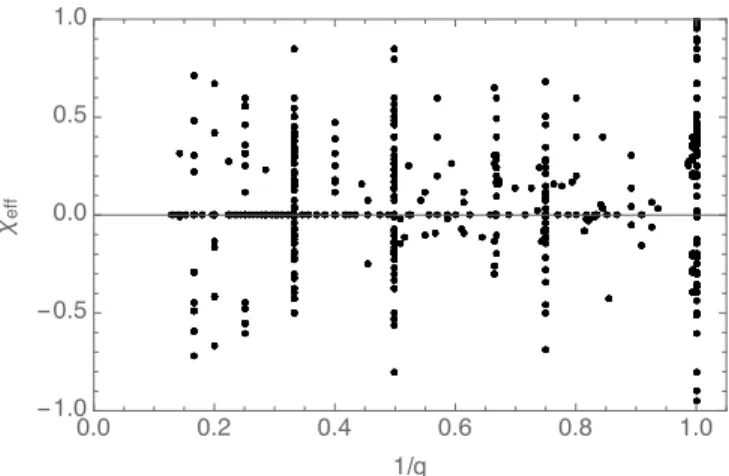
FIG. 1: NR template bank: An illustration of all the simulations used in this study in the 2D space of1/qandχeff [Eq. (2)]. Com-bined with our interpolation methods, the wide range of mass ratios and spins represented in this illustration allow us to reproduce binary parameters for much of the parameter space.
parameters
χi=Si/m2i. (1)
wherei = 1,2indexes the component black holes in the bi-nary. With regard to spin, we define another dimensionless parameter that is a combination of the spins [8–10]:
χeff = (S1/m1+S2/m2)·L/M.ˆ (2) Figure 1 illustrates our NR template bank, with each simu-lation represented as a point in theχeff, q plane. Finally we quantify the duration of each simulation signal by a dimen-sionless parameterM ω0, corresponding to the dimensionless starting binary frequency measured at infinity.
For a given simulation, the GW strain h(t, r,nˆ) can be characterized by a spin-weighted spherical harmonic decomposition at large enough distance: h(t, r,ˆn) = Σl≥2Σlm=−lhlm(t, r)−2Ylm(ˆn). In this expression,nˆis
char-acterized by polar anglesι,−φref; see [11]. For the majority of sources, the (2,±2) mode dominates the summation and can adequately characterize the observationally-accessible ra-diation in any direction to a relative good approximation; how-ever, other higher modes can often contribute in a signifi-cant way to the overall signal [12]. More exotic sources (i.e. high mass ratio and/or precessing, high spins) have significant power in higher modes [13–17].
B. Simulations used
In this work, we use a wide parameter-range of NR simu-lations similar to the set used in [6]. We use all of the 300 public and 13 non-public SXS simulations for a total of 313 [18]. From the RIT group, we use all 126 public and 281 non-public simulations to bring the total contribution up to 407 [19]. We also use a total of 282 simulations provided from the GT group [20]. Including all the contributions from these three groups, we have a total NR template bank of 1002 sim-ulations. Figure 1 shows all the NR simulations in the 2D parameter space ofχeff, as defined in Eq. (2), vs1/qi.e. the mass ratio. All these simulations have already been published and were produced by one of three familiar procedures, see Appendix A in [6] for more details for each particular group.
From these simulations, we selected 12 simulations to focus on as candidate synthetic sources. Table I shows the specific simulations used, specifying the mass ratio (q >1), compo-nent spins of each BH, and total mass. To simplify the process of referring to these heterogeneous simulations, in the last col-umn we assign a shorthand label to each one. These candi-dates have a variety of mass ratios and spins including zero, aligned, and precessing systems from different NR groups. The first three simulations (RIT-1a,-1b, and -1c) have iden-tical initial conditions/parameters, carried out with different simulation numerical resolution. In many of the validation studies, RIT-1a is used; this is a GW150914-like simulation with comparable masses and anti-aligned spins. We use this simulation for its relative simplicity (higher order modes start to become important at the total mass we’ll scale the simu-lation to, namely70M) and to relate it to our similar work done on the real event GW150914.
In this paper, we present 3 end-to-end studies of our param-eter estimation method using data from synthetic sources. We use: a zero spin q=1.0 NR simulation (SXS-1) to show that the method recovers the parameters for the most basic source, an aligned spin GW150914-like simulation (SXS-0233) to show that higher order modes and therefore NR is needed to op-timally recover the parameters even with aligned spin cases, and a precessing source (SXS-0234v2) to show our method arrives at reasonable conclusions for any heavy, comparable-mass binary system with generic spins.
C. Extracting asymptotic strain fromψ4(r, t)
From our large and heterogeneous set of simulations, we need to consistently and reproducibly estimaterhlm(t). Many
gen-eral methods for strain estimation exist; see the review in [21]. The method adopted here must be robust, using the minimal subset of all groups’ output; function with all simulations, precessing or not; and rely on only knowledge of asymptotic proper-ties, not (gauge-dependent) information about dynamics. For these reasons, we implemented our own strain reconstruction and extrapolation algorithm, which as input requires onlyψ4,lm(t)on some (known) code extraction radius. This method combines
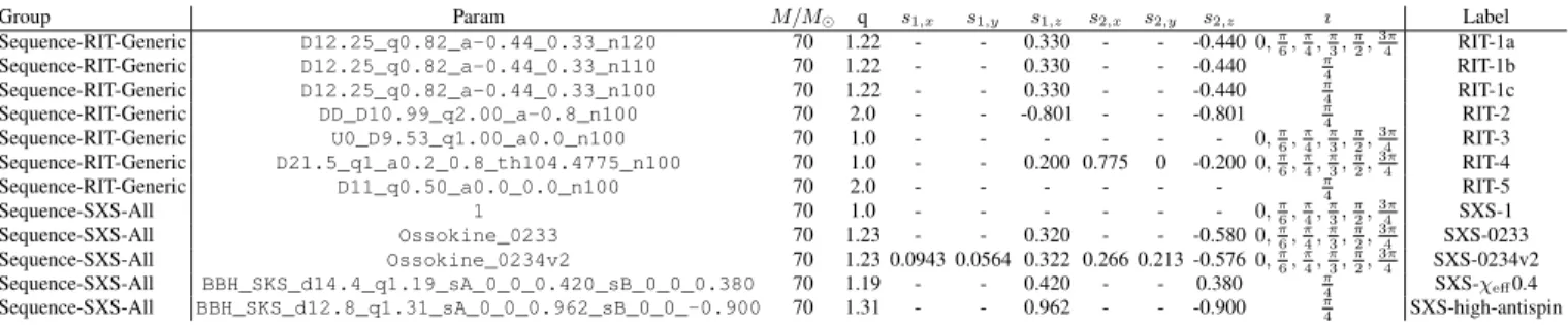
Group Param M/M q s1,x s1,y s1,z s2,x s2,y s2,z ı Label Sequence-RIT-Generic D12.25_q0.82_a-0.44_0.33_n120 70 1.22 - - 0.330 - - -0.4400,π 6, π 4, π 3, π 2, 3π 4 RIT-1a Sequence-RIT-Generic D12.25_q0.82_a-0.44_0.33_n110 70 1.22 - - 0.330 - - -0.440 π 4 RIT-1b Sequence-RIT-Generic D12.25_q0.82_a-0.44_0.33_n100 70 1.22 - - 0.330 - - -0.440 π 4 RIT-1c Sequence-RIT-Generic DD_D10.99_q2.00_a-0.8_n100 70 2.0 - - -0.801 - - -0.801 π 4 RIT-2 Sequence-RIT-Generic U0_D9.53_q1.00_a0.0_n100 70 1.0 - - - 0,π 6, π 4, π 3, π 2, 3π 4 RIT-3 Sequence-RIT-Generic D21.5_q1_a0.2_0.8_th104.4775_n100 70 1.0 - - 0.200 0.775 0 -0.2000,π 6, π 4, π 3, π 2, 3π 4 RIT-4 Sequence-RIT-Generic D11_q0.50_a0.0_0.0_n100 70 2.0 - - - π 4 RIT-5 Sequence-SXS-All 1 70 1.0 - - - 0,π 6, π 4, π 3, π 2, 3π 4 SXS-1 Sequence-SXS-All Ossokine_0233 70 1.23 - - 0.320 - - -0.5800,π 6, π 4, π 3, π 2, 3π 4 SXS-0233 Sequence-SXS-All Ossokine_0234v2 70 1.23 0.0943 0.0564 0.322 0.266 0.213 -0.5760,π 6, π 4, π 3, π 2, 3π 4 SXS-0234v2 Sequence-SXS-All BBH_SKS_d14.4_q1.19_sA_0_0_0.420_sB_0_0_0.380 70 1.19 - - 0.420 - - 0.380 π 4 SXS-χeff0.4 Sequence-SXS-All BBH_SKS_d12.8_q1.31_sA_0_0_0.962_sB_0_0_-0.900 70 1.31 - - 0.962 - - -0.900 π 4 SXS-high-antispin
TABLE I:Synthetic sources: A list of the synthetic sources used in our mismatch studies and end-to-end runs. These are done at different inclinations and with higher order modes. All synthetic sources are performed using the same SNR (20) and the same extrinsic parameters: GPS time109s; RA=0; DEC=3.1; and line of sight relative to the NR simulation characterized by Euler anglesι, φ, ψwithιprovided in the table andφ=ψ= 0.
Specifically, we extractrh(t)at infinity fromψ4(r, t)at finite radius using a perturbative extrapolation technique based on Eq. (29) in [22], implemented in the fourier domain and using a low-frequency cutoff [23]. Specifically, iffminis identified as the minimum frequency content for the mode, we construct the gravitational wave strain fromψ4at a single finite radius from
r˜hlm(f) = ˜ ψ4,lm (iω)2(1−2M/r)[1− (`−1)(`+ 2) 2r 1 iω + (`−1)(`+ 2)(`2+`−4) 8r2 1 (iω)2] + ˜ ψ4,l+1,m (iω)2 2ia (`+ 1)2 s (`+ 3)(`−1)(`+m+ 1)(`−m+ 1) (2l+ 1)(2l+ 3) [iω− `(`+ 3) r ] −ψ˜4,l−1,m (iω)2 2ia (`)2 s (`+ 1)(`−2)(`+m)(`−m) (2l−1)(2l+ 1) [iω− (`−2)(`+ 1) r ] (3)
where the effective frequency is implemented as
iω=i2πsign(f)max(|f|, fmin) (4) and whereais an estimate for the final black hole spin. This method nominally introduces an obvious obstacle to practical calculation: the last two terms manifestly require an estimate ofaand are tied to a frame in which the final black hole spin is aligned with our coordinate axis. In practice, the two spin-dependent terms are small and can be safely omitted in most practical calculations; moreover, each group provides a suitable estimate for the final state. We will clearly indicate when these terms are incorporated into our analysis in subsequent discussion.
When implementing this procedure numerically, we first cleanψ4,lmusing pre-identified simulation-specific criteria to
elim-inate junk radiation at early and late times, tapering the start and end of the signal to avoid introducing discontinuities. For example, for many simulations and for all modes, any content inψ4,lmprior tot≤r+t0was set to zero, for some suitablet0 (fixed for all modes); subsequently, to eliminate the discontinuity this choice introduces, each mode was multiplied by a Tukey window chosen to cover 5% of the remaining waveform duration. Similarly, all data after a mode-dependent timetewas set to
zero, where the timetewas identified via the first time (after the time where|ψ4,22|is largest) wherer|ψ4,lm|fell below a fixed,
mode-independent threshold. To smooth discontinuity, a cosine taper was applied at the end, with duration the larger of either 15 M or 10% of the remaining post-coalescence duration, whichever is larger.
The Fourier transform implementation includes additional interpolation/resampling and padding. First, particularly to enable non-uniform time-sampling, each mode is interpolated and resampled to a uniform grid, with spacing set by the time-sampling rate of the underlying simulation. In carrying out this resampling, the waveform is padded to cover a duration2T + 100M, whereT is the remaining duration of the (2,2) mode after the truncation steps identified above. To simplify subsequent visual interpretation and investigation, the padding is aligned such that the peak of the (2,2) mode occurs near the center of the interval (t= 0).
Finally, the characteristic frequencyM fmin,(l,m) is identified from the starting frequency of eachψ4,lm. In cases where the
starting frequency cannot be reliably identified (e.g., due to lack of resolution), the frequency is estimated from the minimum frequency of the 22 mode as|m|fmin,(2,2)/2.1 In Section IV B we will demonstrate the reliability of this procedure to extract
1This fallback approximation is not always appropriate for strongly
precess-ing systems. However, for strongly precessprecess-ing systems, the relevant start-ing frequency can be easily identified.
h(t)fromψ4.
D. Framework for directly comparing simulations to observations I: Single simulations
In this section, we briefly review the methods introduced in [11] and [6] to infer compact binary parameters from GW data. All analyses of the data begin with the likelihood of the data given noise, which always has the form (up to normaliza-tion) lnL(λ;θ) =−1 2 X k hhk(λ, θ)−dk|hk(λ, θ)−dkik−hdk|dkik, (5) wherehk are the predicted response of the kthdetector due
to a source with parameters (λ, θ) and dk are the
detec-tor data in each instrument k; λ denotes the combination of redshifted massMz and the numerical relativity
simula-tion parameters needed to uniquely specify the binary’s dy-namics;θrepresents the seven extrinsic parameters (4 space-time coordinates for the coalescence event and 3 Euler an-gles for the binary’s orientation relative to the Earth); and ha|bik ≡
R∞
−∞2df˜a(f)∗˜b(f)/Sh,k(|f|) is an inner product
implied by the kthdetector’s noise power spectrumS h,k(f).
In all calculations, we adopt the fiducial O1 noise power spec-tra associated with data near GW150914 [1]. In practice we adopt a low-frequency cutoff fmin so all inner products are modified to ha|bik≡2 Z |f|>fmin df˜a(f) ∗˜b(f) Sh,k(|f|) . (6)
The joint posterior probability of λ, θ follows from Bayes’ theorem:
ppost(λ, θ) =
L(λ, θ)p(θ)p(λ)
R
dλdθL(λ, θ)p(λ)p(θ), (7)
wherep(θ)andp(λ)are priors on the (independent) variables θ, λ. For eachλ, we evaluate the marginalized likelihood
Lmarg ≡
Z
L(λ, θ)p(θ)dθ (8) via direct Monte Carlo integration, wherep(θ)is uniform in 4-volume and source orientation. To evaluate the likelihood in regions of high importance, we use an adaptive Monte Carlo as described in [11]. We will henceforth refer to the algorithm to “integrate over extrinsic parameters” as ILE. The marginal-ized likelihood is a way to quantify the similarity of the data and template. If we integrate out all the parameters except total mass, we get a curve that looks like Figure 2. Having
lnLin this form is the most useful for our purposes, and plots involvinglnLwill be as a function of total mass.
E. Framework for directly comparing simulations to observations II: Multidimensional fits and posterior distribution
The posterior distribution for intrinsic parameters, in terms of the marginalized likelihood and assumed priorp(λ)on
in-trinsic parameters like mass and spin, is
ppost =
Lmarg(λ)p(λ)
R
dλLmarg(λ)p(λ)
. (9)
As we demonstrate by concrete examples in this work, us-ing a sufficiently dense grid of intrinsic parameters, Eq. (9) indicates that we can reconstruct the full posterior parameter distribution via interpolation or other local approximations. The reconstruction only needs to be accurate near the peak. If the marginalized likelihoodLmargcan be approximated by a d-dimensional Gaussian, with (estimated) maximum value Lmax, then we anticipate only configurationsλwith
lnLmax/Lmarg(λ)> χ2d,/2 (10)
contribute to the posterior distribution at the 1-creditable in-terval, whereχ2d,is the inverse-χ2 distribution. [The prac-tical significance of this threshold will be more apparent in Section III B, which implicitly illustrates it using one dimen-sion.] Since the mass of the system can be trivially rescaled to any value, each NR simulation is represented by particular values for the seven intrinsic parameters (mass ratio and the three components of the spin vectors) and is represented by a one-parameter family of points in the 8-dimensional parame-ter space of all possible values ofλ. Given our NR archive, we evaluate the natural log of the marginalized likelihood as a function of the redshifted masslnLmarg(Mz). As in [6], our
first-stage result is this function, explored almost continuously in mass and discretely as our fixed simulations permit. This information alone is sufficient to estimate what parameters are consistent with the data: for example, using a cutoff such as Eq. (10), we identify the masses that are most consistent for each simulation.
As demonstrated first in [6] and explored more systemati-cally here, this likelihood is smooth and broad extending over many NR simulations’ parameters. As a result, even though our function exploration is a restricted to a discrete grid of NR simulation values, we can interpolate between simulations to reconstruct the entire likelihood and hence entire posterior. We can do this because of the simplicity of the signal, which for the most massive binaries involves only a few cycles. More broadly, our method works because many NR simulations pro-duce very similar radiation, up to an overall mass scale; as a result, as has been described previously in other contexts [24], surprisingly few simulations have been needed to explore the model space (e.g., for nonprecessing binaries).
Finally, as we demonstrate repeatedly below by example,
lnLmarg is often well approximated by a simple low-order series, typically just a quadratic. Moreover, for the short GW150914-like signals here, many nonprecessing simula-tions fit both observasimula-tions and even precessing simulasimula-tions fairly well. As a result, we employ a quadratic approximation tolnLmarg near the peak under the restrictive approximation that all angular momenta are parallel using information from only nonprecessing binaries. Using this fit, we can estimate
lnLmarg for all masses and aligned spins and therefore esti-mate the full posterior distribution. Section IV B in [6] gives the results of this method based on the LIGO data containing GW150914. In this work, we apply this method to a larger set of examples.
III. DIAGNOSTICS
Many steps in our procedure to compare NR simulations to GW observations can introduce systematic error into our in-ferred posterior distribution. Sources of error include the nu-merical simulations’ resolution; waveform extraction; finite duration; Monte Carlo integration error; the finite, discrete, and sparsely spaced simulation grid; and our fit to said grid. In the following sections, we describe tools to characterize the magnitude and effect of these systematic errors. First and foremost, we introduce the broadly-usedmatch, a complex-valued inner product which arises naturally in data analysis and parameter inference applications. Following many previ-ous studies [25], we review how systematic error shows up as a mismatch and parameter bias. Second, we describe an anal-ogy to the match which uses our full multimodal infrastructure and is more directly connected to our final posterior distribu-tion: the marginalized likelihood versus masslnLmarg(M), or equivalently (one-dimensional) posterior distribution im-plied by assuming the data must be drawn from a specific sim-ulation up to overall unknown mass and orientation. Due to systematic error, the inferred one-dimensional distribution (or match versus mass) may change, both globally and through any concrete confidence interval (CI) derived from it. To ap-propriately quantify the magnitude of these effects, we intro-duce two measures to compare similar distributions. On the one hand, any change in the 90% CI provides a simple and easily-explained measure of how much an error changes our conclusions. On the one hand, the KL divergence(DKL) gives a simple, well-studied, theoretically appropriate, and numer-ical measure of the difference between two neighboring dis-tributions. In this section we describe these diagnostics and illustrate them using concrete and extreme examples to illus-trate how a significant error propagates into our interpretation.
A. Inner products between waveforms: the mismatch
The match is a well-used and data-analysis-driven tool to compare two candidate GW signals in an idealized setting. Unlike most discussions of the match, which derive them from the response of a single idealized instrument, we follow [26] and work with the response of an idealizedtwo-detector in-strument, with both co-located identical interferometers ori-ented at45o relative to one another, and the source located
directly overhead this network.2As is well-known, the match
2Equivalently, we work in the limit of many identical detectors, such that
the network has equal sensitivity to both polarizations for all source
prop-arises naturally in the likelihood of a candidate signal, given known and noise-free data – or, in the notation of this work, from Eq. (5) restricted to this idealized network, settingdto h0=h(t, λ0)andh(λ, θ) =h: lnL=−1 2{hh−h0|h−h0i − hh0|h0i} =−1 2{hh|hi −2<hh0|hi}, (11)
where<is the real part. Againha|biis the complex overlap (inner product) between two waveforms for a single detector as shown in Eq. (6); the GW strainh=h+−ih×contains two polarizations, and is assumed to propagate from directly over-head the network; the likelihood reflects the response of both detectors’ antenna response and noise. Eq. (11) is slightly different than the the likelihood obtained in Eq. (17) of [26] by an overall constant. What we use, described in [27], is the likelihood ratio (divided by the likelihood of zero signal). If we add this constant back into the equation, we recover Eq. (17) from [26]:
lnLsingle=−
1
2{hh0|h0i+hh|hi −2<hh0|hi}. (12)
This single-detector likelihood depends on the parametersλ, θ of handλo, θ0 of h0. For the purposes of our discussion, we will include “systematic error” parameters that enhance or change the model space inλ(e.g., changes in simulation resolution).
The parameters which maximize the likelihood identify the configuration of parameters that makehmost similar toh0. For a fixed emission direction from the source, three key pa-rameters inθ dominate howhcan be changed to maximize the likelihood: the event timetevent; the source luminosity distanceDL; and the polarization angleψ, characterizing
ro-tations of the source (or detector) about the line of sight con-necting the source and instrument. In terms of these parame-ters,
h=e−2iψDL,ref DL
href(t−tevent|λ, θrest) (13)
wherehref is the value ofhatDL =DL,ref, tevent= 0, and ψ= 0andθrest denotes the four remaining extrinsic param-eters besides these three. As noted in [26], a change of the polarization angleψcorresponds to a rotation of the argument of the complex strain function,h(ψ) = e−2iψh(ψ = 0). As a result, maximizing the likelihood versusψcorresponds to choosing a phase angle sohh|h0iis purely real:
maxψhh0|hi=|hh0|hi|. (14) Similarly maximizing the likelihood versus distance, the like-lihood becomes
max ψ,DL
lnLsingle=−ρ2(1−P∗). (15)
where in this expressionρ2=hh0|h0i=hh|hiand the func-tionPis P∗(h0, h)≡maxψ |hh0|hi| p hh0|h0ihh|hi , (16)
This partially-maximized likelihood depends strongly on the event time. If we furthermore maximize over event time, we find the final and important relationships
lnLsingle,max= max
ψ,DL,tevent lnLsingle=−ρ2(1−P), (17) P(h0, h)≡maxψ,tevent |hh0|hi| p hh0|h0ihh|hi . (18)
In the rest of this paper, we will use the mismatchM be-tween two signals:
M(h0, h) = 1−P(h0, h). (19) Because of its form – an inner product – the mismatch identi-fies differences between the two candidate signals; substitut-ing this expression into the maximized ideal-detector likeli-hood [Eq. (17)] yields:
lnLsingle,max=−ρ2M. (20) As the above relationships make apparent, a candidate sig-nal hwhich has a significant mismatch cannot be scaled to resembleh0and therefore must be unlikely. This relationship has been used to motivate simple criteria to characterize when two signalsh, h0are indistinguishable (or, conversely, distin-guishable); working to order of magnitude [cf. Eq. (10)], two signals are indistinguishable if [28–31]
M ≤ 1
ρ2. (21)
In this work, we apply the match criteria to assess when two simulations of the same or similar parameters (or the same simulation at a different mass) can be distinguished from a reference configuration.
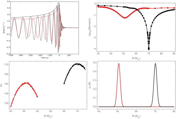
As a concrete example, discussed at greater length in Sec-tion III E, the top-right panel in Figure 3 shows two plots of mismatch versus total mass. In the black curve, we calculate the match of two identical waveforms from the RIT-1a sim-ulation: one set at a fixed total massM = 70Mwhile the other changes over a given mass range. At the true total mass, the mismatch goes to zero. For comparison, the red curve in that figure shows the mismatch between another simulationh and a fixed RIT-1a (h0), versus total mass forh. As illustrated in the top-left panel of Figure 3, the two simulations are not identical; hence, the mismatch in the top-right panel between handh0never reaches zero. Moreover, due to differences in the sourcehoand template familyh, the location of the
mini-mum mismatch and hence best fit occurs at a different, offset total mass, close to50M.
As the reader will see in subsequent sections, we can also calculate the mismatch as a function of particular properties of NR simulations to see how much error is introduced, see Section IV.
B. Marginalized likelihood versus mass
Another simple diagnostic is the resultlnLmarg(M)for a single simulation on some reference data (e.g., the simulation itself, or a signal with comparable physical origin). This func-tion enters naturally into our full parameter estimafunc-tion cal-culation; therefore, it allows us to test all of the quantities that influence our principal result directly including NR res-olution, extraction radius, etc. as described below. For sim-plicity, as computed for the purposes of this test, this function depends on part (onlyl ≤2modes) of the NR radiation and the data. Figure 2 shows a null example run with RIT-1a, a GW150914-like simulation, as a source compared against it-self. As previous work from both real LIGO and synthetic data has suggested,lnL(M)can be well-approximated by a locally quadratic fit (see Section III D for a more in-depth dis-cussion of this example).
C. Probability Density Function/KL Divergence
To quantitatively assess whether two given versions of lnL(M) are demonstrably different, we employ an observationally-motivated diagnostic to prioritize agreement in regions with significant posterior support. Motivated by the applications we perform when comparing results of this kind, we translatelnL(M)into a probability distribution (i.e., as-suming all other parameters are fixed):
pc(M) = 1
R
dM elnLe
lnL. (22)
In practice, this distribution is always extremely well approx-imated by a gaussian, so we can further simplify by char-acterizing any 1d distribution by its meanM∗ and variance
1/ΓM M =σ2∗. Using this ansatz, we can therefore define a quantity to assess the difference between any pair of results forlnL(M). In this work, we use the KL divergence between these two approximately-normal distributions:
DKL(p∗|p) = Z dxp(x) lnp(x)/p∗(x) = ln σ σ∗ −1 2+ (¯x−x¯∗)2+σ∗2 2σ2 . (23)
We also will plot the derived PDF pc(M) and evaluate the
implied 1D 90% CI derived from it.
The implications of a significant disagreement for this di-agnostic – already illustrated via high mismatch in Figure 3 – can be clearly seen in the 1D posterior distributions derived from the fit oflnLmarg(M)as shown in Figure 3 and Figure 4. Loosely following the work in [25] for estimating parameter errors due to mismatch, we expect the parameter error will be a significant fraction of the statistical error. Using the notation above and approximatingP '1−1
2Γ¯xxδx
2for some nomi-nal perturbed parameterx, we estimate the statistical error to beσx,stat '1/ρ
√
�� �� �� �� �� �� �� �� ��� ��� ��� ��� ��� ��(�⊙) ��� �� �� �� �� �� ��� ��� ��� ��� ��� �(�⊙) �� ( � )
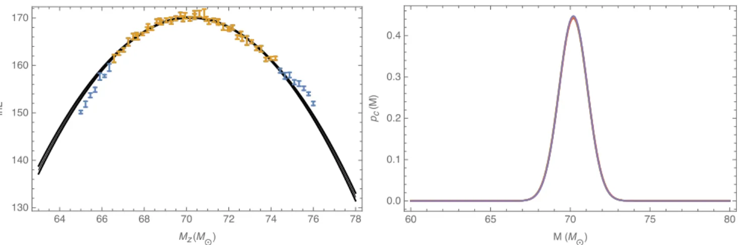
FIG. 2: Example oflnLmarg(M): comparing a simulation to itself: Left panel: Blue and yellow points (with error bars) show results of evaluatinglnLmarg(M)with RIT-1a as a source compared to itself. The shaded region is derived by fitting a quadratic to these data via least-squares [Eq. (25)], providing a mean and confidence interval (shown). The reference source has total massM = 70Mand an inclinationı= 0.785; all calculations are carried out usingfmin= 30Hz. This curve will be duplicated as a black curve in the right panel from Figure 3 and left panel from Figure 4. Right panel: Nominal one-dimensional posterior distributions [Eq. (22)] derived from the fit to left. This figure shows five examples, randomly drawn from the fit coefficient distribution derived by least squares, drawn to exemplify the propagated systematic uncertainties due to Monte Carlo integration error. For studies similar to this one (i.e., high-mass investigations where direct comparison to numerical relativity is most appropriate), this figure suggests that Monte Carlo error is much smaller than the posterior width (i.e., has little relevance given the substantial statistical uncertainty introduced by the limited number of GW cycles available for comparison from short NR simulations).
parameter biases, similar changes in likelihood occur when δx' 1
¯ Γ1xx/2
M1/2;
(24)
however, much more detailed calculations is presented in [25]. The above relationship illustrates how a high mismatch causes a deviation in the lnLmarg(M) curve as well as its corre-sponding posterior distribution. Figure 3 show a comparison between two waveforms from RIT-1a and RIT-2 (red curve). With significantly different parameters (see Table I), the mis-match is significantly high. This causes a radical shift in the
lnLmarg(M) result as well as its corresponding PDF com-pared to to it’s true value. This example will be described in greater detail in Section III E.
D. Example 0: Null test/Impact of Monte Carlo Error
To illustrate the use of these diagnostics, we first apply them to the special case where the data contains the response due to a known source. In this case, by construction, the match will be unity when using the same parameters. Fol-lowing a similar procedure to that we would apply if we didn’t know the source mass, we can also plot the mismatch hhA(M)|hA(M∗)i/||hA(M)||||hA(M∗)||. Referring to the notation in Eq. (16), we assign the RIT-1a waveform to h0 = hRIT−1a(source) and again the RIT-1a waveform to
h = hRIT−1a (template). This plot can be seen in any of
the following examples as the black curve (top-right panels from Figure 3 and Figure 4). It has a peak value of unity (not plotted) and rapidly falls as one moves away from the mass corresponding to the peak match value. The left panel
of Figure 2 shows the log likelihood lnLmarg provided by
ILEas a function of mass. From here we fit a local quadratic to thelnLmarg close to the peak. Using the fit, we generate five random samples and use them for subsequent calculations (i.e. 1D distributions). We derived a 1D distribution using Eq. (22).
First and foremost, these figures illustrate the relationships between the three diagnostics. As suggested by Eq. (20), the match and log likelihoodlnLmargare nearly proportional up to an overall constant. Second, as required by Eq. (22), the one-dimensional posterior is proportional toLmarg. This vi-sual illustration corroborates our earlier claim implicit in the left panel of Figure 2: only the part oflnLmarg within a few of its the peak value contributes in any way to the posterior distribution and to any conclusions drawn from it (e.g., the 90% CI).
Each evaluation of the Monte Carlo integral has limited accuracy, as indicated in Figure 2. By taking advantage of many evaluations of this integral, we dramatically reduce the overall error in the fit. To estimate the impact of this un-certainty, we use standard frequentist polynomial fitting tech-niques [32] to estimate the best fit parameters and their un-certainties (i.e., of a quadratic approximation tolnLnear the peak): iflnLmarg =PαλαFα(Mz)andγkk = 1/σ2kis an
inverse covariance matrix characterizing our measurement er-rors, then the best-fit estimate forlnLmarg and its variance is
lnLmarg,est=F(FTγF)−1γy (25a)
Σ(x) =Fα(x)[(FTγF)−1]αβFβ(x) (25b)
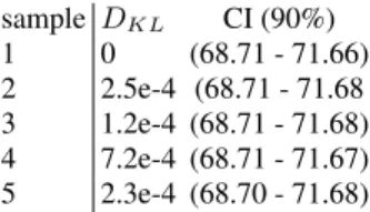
sample DKL CI (90%) 1 0 (68.71 - 71.66) 2 2.5e-4 (68.71 - 71.68 3 1.2e-4 (68.71 - 71.68) 4 7.2e-4 (68.71 - 71.67) 5 2.3e-4 (68.70 - 71.68)
TABLE II:KL Divergence and 90% CI between different samples from the null test fit: This table shows theDKLand 90% CI for five different sample PDFs. TheDKLwas calculated comparing the 1D distributions to the first sample (i.e.DKLfor sample 1 is zero). The CI are also given to show the change between them. Both diagnostics suggest the distributions are nearly indistinguishable.
data points andF is a matrix representing the values of the basis functions on the data points:Fα(xk). The left panel of
Figure 2 shows the 90% CI derived from this fit, assuming gaussian errors.
To translate these uncertainties into changes in the one-dimensional posterior distribution pc, we generate random
draws from the corresponding approximately multinomial dis-tribution for fit parameters; and thereby generate random sam-ples and hence one-dimensional distributions forpc(M)
con-sistent with different realizations of the Monte Carlo errors. The right panel of Figure 2 shows five random samples from the fit in the left panel. This figure demonstrates this level of Monte Carlo error, by design, has negligible impact on the posterior distribution. To quantify the impact of Monte Carlo error on the posterior, we calculate the KL Divergence from Eq. (23). In all cases, the KL divergence was small, of order
10−4, see Table II for more details onDKLand the 90% CI.
In Section IV A, we further verify this conclusion by repeating our analysis many times.
E. Example 1: Two NR simulations with different parameters/Illustrating how sensitively parameters can be
measured
In this example we compare two NR simulations with sig-nificantly different parameters to demonstrate how our diag-nostics handle waveforms of extreme contrast. The two NR simulations used are RIT-1a and RIT-2. As shown in Table I, these simulations are both aligned spin with different magni-tudes withq= 1.22andq= 2.0respectively. To illustrate the extreme differences between the radiation from these two sys-tems, the top-left panel of Figure 3 shows the two simulations’ rh(t).
Our three diagnostics equally reveal the substantial differ-ences between these two signals. To be concrete, since these diagnostics treat data and models asymmetrically, we operate on synthetic data containing RIT-1a with inclinationı=π/4
in these applications. First, the top-right panel of Figure 3 shows the results of our mismatch calculations. The black curve is the same null test mismatch calculation as in the top-right panel of Figure 4: it has a narrow minimum (of zero) at the true binary mass (70M). For the red curve, we calculate the mismatch while holding RIT-2 at a fixed mass and chang-ing the mass of RIT-1a. Uschang-ing the notation in Eq. (16), we
as-ILErun (source/template) DKL CI (90%) RIT-1a/RIT-1a 0.0 (68.8 - 71.4) RIT-2/RIT-1a 288.8 (49.3 - 52.0)
TABLE III:KL Divergence and 90% CI between two NR simu-lations with different parameters: This table shows theDKLand 90% CI between: RIT-1a/RIT-1a and RIT-1a/RIT-2. TheDKLwas calculated comparing the 1D distributions to RIT-1a/RIT-1a distribu-tion (notice itsDKL is zero i.e. they’re identical). The CI are also given to show the difference between these two distributions.
sign the RIT-2 waveform toh0=hRIT−2(fixed mass atM =
70M) and the RIT-1a waveform toh=hRIT−1a(changing mass). In this case, the match does not reach unity, differing by a few percent, while the peak value occurs at significantly offset parameters (here, in total mass). Second, the bottom-left panel of Figure 3 shows the results forlnLmarg(M), us-ing these two NR simulations to look at the same stretch of synthetic data including our local quadratic fit to them. Third, the bottom-right panel of Figure 3 shows the implied one-dimensional posterior distribution derived from our fits. There is a clear shift in total mass with the null test again peaking around70Mand this example’s peak around50M. There are also orders of magnitude difference between thelnLmarg of the two cases. These diagnostics show something that could be seen just by looking at the waveforms; however, we now have some idea on how major differences propagate through our diagnostics and how the error in each diagnostic relate to each other. For completeness, we also include theDKL and
CI for these two waveforms in Table III. TheDKLas well as
the CI are both considerably offset, as expected given the two significantly different simulations involved.
Finally, the parameter shift seen above is roughly consis-tent in magnitude with what we would expect for such an ex-treme mismatch error, given the SNR and match: we expect using Eq. (24)δM ' σMρM1/2 ' 5σM ' 5M (using M = 6×10⁻², ρ = 20andσ
M = 1.1M), or a shift in best fit of several standard deviations and many solar masses. While noticeably smaller than our actual best-fit shift, our re-sult from Eq. (24) provides a valuable sense of the order-of-magnitude biases incurred by specific level of mismatch in general. Moreover, this example is a concrete illustration of the critical need to haveM ≤1/ρ2to insure that any system-atic parameter biases are small and under control.
F. Example 2: Different physics: SEOB vs NR/Illustrating the value of numerical relativity
Several studies have previously demonstrated the critical need for numerical relativity, since even the best models do not yet capture all available physics [33, 34]. For example, these models generally omit higher-order modes, whose omis-sion will impact inferences about the source [35–37].
To illustrate the value of NR in the context of this work, we compare parameter estimation with NR and with an ana-lytic model. In this particular example, we use NR simula-tion RIT-1a including thel ≤ 2 modes (see Table I)
evalu-●●●●●●●●●●●●● ●● ●● ●● ●●●●●●● ●●●● ●●●●●●●●●●● ● ● ● ● ● ● ● ● ●●●●●●●●●●●● ● ● ● ● ● ● ● ● ●● ●● ● ● ● ● ●●●● ●● ●● ●● ●●● ● ● ●● ●●● ●●●●● ●●●●●●● 30 40 50 60 70 80 90 -4 -3 -2 -1 0 M(M⊙) log 10 ( Mismatch ) 45 50 55 60 65 70 130 140 150 160 170 M(M⊙) lnL 40 50 60 70 80 0.0 0.1 0.2 0.3 0.4 0.5 M(M⊙) pc ( M )
FIG. 3: Example 1-Assessing differences between two NR simulations with different parameters: Two representations of the different predictions of RIT-1a and RIT-2, which are aligned spin binaries with mass ratiosq= 1.22andq= 2.0respectively, illustrating how dramatic differences propagate into our diagnostics. Top-left panel: The strain along a line of sight inclined atι= 0.785and evaluated for a total massM = 70M, with RIT-1a in black and RIT-2 in red. Top-right panel: The mismatch between synthetic data and candidate templates as a function of the template’s mass. In both cases, the RIT-1a simulation is used as the template (i.e., ashin Eq. (16)). For the black curve, RIT-1a for a70Mbinary is also used as the source (i.e.,h0 =hRIT−1a). For the red curve, the source is RIT-2 set at M=70M. while RIT-1a has a changing massBottom-left panel: Points show the marginalized likelihood versus total mass calculated by applying the same template simulation (RIT-1a) to two different sources: RIT-1a in black and RIT-2 in red. Each source has fixed massM = 70Mand inclinationı= 0.785; as in Figure 2, we evaluateLusing a low-frequency cutofffmin= 30Hz. For context, red and black solid curves show a corresponding quadratic least-squares fit to these data.Bottom-right panel: The corresponding one-dimensional posteriorspc(M)[Eq. (22)]. Both bottom panels illustrate how an ill-suited simulation with large mismatch (i.e., the red curve) correlates with a drastic shift in parameters (here, total mass) relative to the true best-fit solution (here, the black curve), [see Eq. (24)]. Also, the ill-matched simulation cannot recover all the information available to the true solution, so the peaklnLmargfor the red curve is substantially lower ('20) than the peak of the black curve.
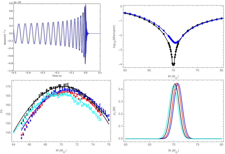
ated along an inclinationι = π/4. Using this line of sight and our fiducial mass (M = 70M), higher harmonics play a nontrivial role. For our analytical model, we use an Effective-One-Body model with spin (SEOBNRv2), described in [38], which was one of the models used in the parameter estima-tion of GW150914 [39] and which was recently compared to this simulation [33]. The top-left panel of Figure 4 shows the time-domain strains from the NR simulation and SEOBNRv2 with the same parameters. To better quantify the small but vi-sually apparent difference in the two waveforms, we use the diagnostics described earlier on these two waveforms.
One way to characterize the differences in these waveforms
is the mismatch [Eq. (16)]. In the top-right panel of Figure 4, we calculate the mismatch by holding the SEOBNRv2 form at a fixed mass while changing the mass of the NR wave-form shown in blue. Referring to the notation in Eq. (16), we assign the SEOBNRv2 waveform toh0 = hSEOBNRv2 and the RIT-1a waveform toh = hRIT−1a. For comparison, a mismatch calculation was done with the null test from Sec-tion III D (RIT-1a compared to itself) shown here in black. Two differences between the two curves are immediately ap-parent. First, the blue curve does not go to zero; the mismatch is a few times10−3, significantly in excess of the typical ac-curacy threshold [Eq. (21), evaluated atρ = 25]. Second,
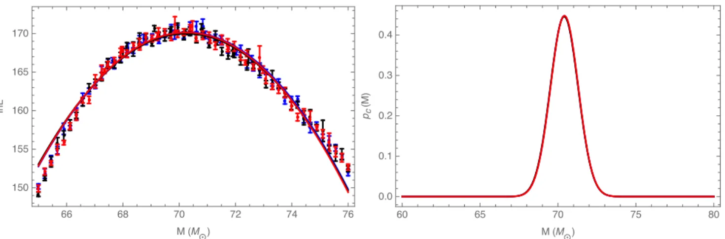
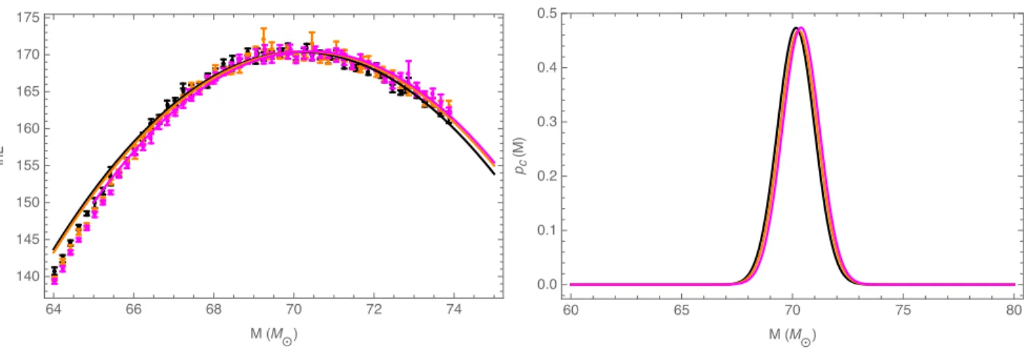
● ● ● ● ● ● ● ● ● ● ●● ●● ● ● ● ● ● ●●● ●● ●● ●● ●●● ● ● ● ● ● ● ● ● ● ● ● ● ● ● ● ● ● ● ● ●●●●●●●●●●●●●●●●●●●●●●● ● ● ● ● ● ● ● ● ● 60 65 70 75 80 -4 -3 -2 -1 0 M(M⊙) log 10 ( Mismatch ) 64 66 68 70 72 74 76 145 150 155 160 165 170 M(M⊙) lnL 60 65 70 75 80 0.0 0.1 0.2 0.3 0.4 M(M⊙) pc ( M )
FIG. 4: Example 2-Assessing differences in SEOB and NR waveforms that have the same parameters: This figure shows how subtle differences between an NR solution and an approximation to GR (here, EOB) can propagate into mismatch and parameter estimation. These two companion figures follow the pattern of Figures 3. Top-left panel: The black and blue curves show the strain evaluated from RIT-a and SEOBNRv2, respectively, for a source with identical parameters. Source parameters and strain results for the black curve are identical to Figure 3 (e.g.,ι=π/4).Top right-panel: Following the top-right panel of Figure 3, this figure shows the match between the two waveforms on the top-left with the corresponding template from RIT-1a.Bottom-left: The marginalized likelihoodlnLmargfor the two waveforms shown above, evaluated usingbothRIT-1a and SEOBNRv2 as templates: NR source compared to same NR template in black; the SEOBNRv2 source to a SEOBNRv2 template in red; the SEOBNRv2 source to a NR (RIT-1a) template in blue; and the NR (RIT-1a) source to a SEOBNRv2 template in cyan.Bottom-right: The one-dimensional posterior distributionspc(M)derived from the quadratic fits shown in the bottom-left. Both bottom panels show a clear change along the total mass for SEOBNRv2 sources. The NR/NR comparison has the highestlnLmargwith with a corresponding total mass∼70M. The NR/SEOBNRv2 template curve correctly finds the total mass∼70M; however, thelnLmarg is orders of magnitudes different than the null example. The differences between NR simulations and the SEOBNRv2 model is significant for parameter estimation.
the minimum occurs at offset parameters. The best-fit offset and mismatch are qualitatively consistent with the naive esti-mate presented earlier: a high mismatch yields a high change in total mass [see Eq. (24)]. This simple calculation illustrates how mismatch could propagate directly into significant biases in parameter estimation.
Another and more observationally relevant way to char-acterize the differences between these two waveforms is by carrying out a full ILE based parameter estimation calcula-tion. We carry out four comparisons: the null test (a NR source compared to same NR template (black)); the SEOB-NRv2 source compared to a SEOBSEOB-NRv2 template (red); the NR source compared to a SEOBNRv2 template (cyan); and
an SEOBNRv2 source compared to a NR template (blue). The bottom panels of Figure 4 shows both the underlying
lnLmarg(M) results; our quadratic approximations to the data; and our implied one-dimensional posterior distributions [Eq. (22)]. AllILEcalculations were carried out withfmin=
30Hz. All four likelihoods lnLmarg and posterior distribu-tionspcare manifestly different, with generally different peak
locations and widths. Table IV quantifies the differences be-tween the possible four configurations, usingDKL and 90%
CI. The DKL was always calculated by comparing one of
them to the NR/NR case. These systematic differences exist even without higher modes, whose neglect will only exacer-bate the biases seen here.
ILEconfiguration (source/template) DKL CI (90%) SEOB/SEOB 0.086 (69.2 - 72.1) SEOB/RIT-1a 0.25 (69.4 - 72.4) RIT-1a/RIT-1a 0 (68.8 - 71.8) RIT-1a/SEOB 0.050 (68.5 - 71.5)
TABLE IV:KL Divergence and 90% CI between SEOB and NR: This table shows theDKLand 90% CI for the four different config-urations using SEOBNRv2 and NR as sources and templates. The
DKL was calculated comparing the 1D distributions to the NR/NR case (notice itsDKLis zero i.e. they’re identical). The CI also given to show the change between them. Based on theDKL results, the 1D posteriors are similar but not exactly the same distribution. These nontrivial differences affect our parameter estimation results and also change our astrophysical conclusions about the source.
Keeping in mind the two figures adopt a comparable color scheme, the shift in peak value and location between the black and blue curves seen in the bottom panels of Figure 4 can be traced back to the top-right of Figure 4: to a first approxima-tion, systematic errors identified by the mismatch (M) show up in the marginalized likelihood (lnLmarg). Again, based on calculations using Eq. (24), we expect the change in mass location of order unity holding all other things equal, compa-rable to the observed offset.
In many ways, one-dimensional biases shown in the bottom-right panel understatethe differences between these signals: that comparison explicitly omits the peak value of
lnLmarg, which occurs not only at a different location but also with a different value for all four cases. As we would expect, the NR/NR case has the highestlnLmargwith a peak near the true total mass 70M. The NR/SEOB case can also produce a peak near 70M; however, thelnLmargis orders of magni-tude lower, which translates to a lower likelihood that this was in fact the correct template. When performing a full multidi-mensional fit, template-dependent biases in the peak value of
lnLmargcan also impact our conclusions.
To summarize, we have shown that using SEOBNRv2 in place of a more precise solution of Einstein’s equations intro-duces non-negligible systematic errors, of a magnitude com-parable to the statistical error for plausible sources, and that it can impact astrophysical conclusions.
G. Example 3: Signal duration and cutoff
frequency/Illustrating the impact of simulation duration with SEOB
Numerical relativity simulations have finite duration. Until hybrids [40–43] are ubiquitously available, these finite dura-tion cutoffs will impair the utility of direct comparison be-tween data and multimodal NR simulations. To assess this impact of finite simulation duration, we adopt a contrived but easily-controlled approach, using an analytic model where we can freely adjust signal duration. While our specific numeri-cal conclusions depend on the noise power spectrum adopted, as it sets the required low-frequency cutoff, the general prin-ciples remain true for advanced instruments.
In this example, we plot lnLmarg for a fiducial
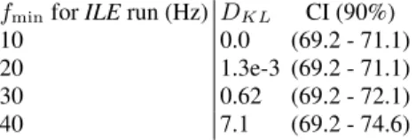
SEOB-fminforILErun (Hz) DKL CI (90%) 10 0.0 (69.2 - 71.1) 20 1.3e-3 (69.2 - 71.1) 30 0.62 (69.2 - 72.1) 40 7.1 (69.2 - 74.6)
TABLE V:KL Divergence and 90% CI of PDFs derived from SEOB sources with different low frequency cutoffs: This table shows theDKLand 90% CI for the four different configurations us-ing SEOBNRv2 source with a set duration of5Hzand compared against SEOBNRv2 templates with different low frequency cutoffs. The DKL was calculated comparing the 1D distributions to the
fmin= 10Hzcase (notice itsDKLis zero i.e. they’re identical). The CI also given to show the change between them. Based on theDKL
results, the 1D posteriors offmin = 10,20Hzseem to be the same distribution; however, they differ significantly tofmin= 30,40Hz.
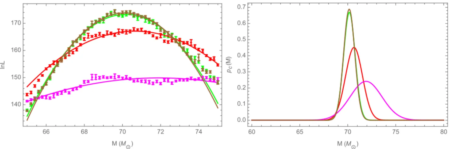
NRv2 source versus itself using different choices for the low-frequency cutoff (and, equivalently, different initial orbital frequencies for the binary). The left panel of Figure 5 shows
lnLmarg versus M. In this figure, the lnLmarg curves for fmin = 10Hzand20Hz(brown and green) are significantly narrower and higher compared to the lnLmarg curves for fmin= 30Hzor40Hz(red and magenta). As described in [6], even though very little signal power is associated with very low frequencies for this combination of detector and source, a significant amount of information about the total mass is avail-able there with all other parameters of the system perfectly known. These differences are immediately apparent in our one-dimensional diagnosticslnLmarg(M)andpc(M), which
are both narrower and more informative when more informa-tion is included (i.e., for lowerfmin). That said, our PSD does not provide access to arbitrarily low frequencies, and the low-est two frequencies have nearly identical posterior distribu-tions, as measured by KL divergence, see Table V. This inves-tigation strongly suggests our analysis could be sharper with longer simulations or hybrids. That said, [6] demonstrated this procedure will, for GW150914-like data and noise, arrive at similar results to an analysis which includes these lower frequencies. As noted in [6], this virtue leverages a fortu-itous degeneracy in astrophysically relevant observables: the limitations of our high-frequency analysis are mostly washed out due to strong degeneracies between mass, mass ratio, and spin.
IV. VALIDATION STUDIES
In this section we self-consistently assess our errors inh(t)
andlnL. Using the diagnostics described above, via targeted one-dimensional studies, we systematically assess the impact of Monte Carlo error; waveform extraction error; simulation resolution; and limited access to low frequency content. We will show via our diagnostics that the effects from these poten-tial sources of error can be either ignored or mitigated (e.g., by a suitable choice of operating point for our analysis pro-cedure, such as a high enough extraction radius). For each potential source of error, we use the KL divergenceDKL[Eq.
poste-66 68 70 72 74 140 150 160 170 M(M⊙) lnL 60 65 70 75 80 0.0 0.1 0.2 0.3 0.4 0.5 0.6 0.7 M(M⊙) pc ( M )
FIG. 5:Example 3-Quantifying the impact of the low-frequency cutoff: Using analytic SEOBNRv2 templates with user-specified starting frequency and length, this figure quantifies the impact of our choice of low-frequency cutoff on parameter estimation. Left panel: Plot of lnLmargversus total mass evaluated using SEOBNRv2 templates with different starting frequencies withfmin= 10Hz(brown),fmin= 20Hz (green),fmin = 30Hz(red), andfmin = 40Hz(magenta). In all cases, the source signal is also SEOBNRv2 using the same parameters as RIT-1a, but starting frequencyfmin= 5Hz.Right panel: The one-dimensional posteriorspc(M)[Eq. (22)] implied by the results to left. As you increase the low frequency cutoff, thelnLmargdecreases significantly, and both the posterior andlnLmargare wider and offset from the true parameters.
Trial DKL CI (90%) v1 0 (68.9 - 71.9) v2 4.8e-5 (68.9 - 71.9) v3 5.6e-5 (68.9 - 71.9)
TABLE VI:KL Divergence and 90% CI between different runs of the same null test.: This table shows theDKL, calculated using Eq. (23) and 90% CI for three different runs of the same configuration as described in Section III D. TheDKLwas calculated comparing the 1D distributions to Trial v1 (notice itsDKLis zero i.e. they’re iden-tical). The CI also given to show the change between them. Based on theDKL results, the 1D posteriors of these different trials are identical.
rior distributionspc(M)[Eq. (22)] derived fromlnLmarg. We will relate our results to familiar mismatch-based measures of error. To be concrete, we will employ a target signal ampli-tude (SNR)ρ= 25, similar to GW150914. For similarly-loud sources, the mismatch criteria [Eq. (21)] suggests any param-eters with mismatch below log10(M) = −2.8 will lead to “statistical errors” (associated with the width of the posterior) will be smaller than systematic biases.
A. Impact of Monte Carlo error
We have already assessed the error from our Monte Carlo integration in Section III D, directly propagating the (assumed correct) Monte Carlo integration error into our fit. To compre-hensively demonstrate the impact of Monte Carlo integration error, we repeat our entire analysis reported in Figure 2 mul-tiple times. Figure 6 shows our directly comparable results; Table VI reports quantitative measures of how these distribu-tions change. Based on these quantities, we conclude the error introduced by our Mont Carlo is negligible. Our results are
consistent with Section III D.
B. Error budget for waveform extraction
While gravitational waves are defined at null infinity, the fi-nite size of typical NR computational domains implies a com-putational technique must identify the appropriate asymptotic radiation from the simulation [44]. This method generally has error, often associated with systematic neglect of near-field physics in the asymptotic expansion used to extract the wave (i.e., truncation error). Our perturbative extrapolation method shares this limitation. As a result, if we decrease the radius at which we extract the asymptotic strain, we increase the error in our approximation. In other words, the mismatch between the waveform extracted atrand some large radius generally decreases withr; the trend of match versusrprovides clues into the reliability of our results.
Figure 7 shows an example of a mismatch between two es-timates of the strain: one evaluated at finite, largest possible radius and one at smaller (and variable) radius. For context, we show the nominal accuracy requirement corresponding to a SNR=25 [see Eq. (21)] as a black dotted line. First and foremost, this figure shows that, at sufficiently high extrac-tion radius, the error introduced by mismatch errors is sub-stantially below our fiducial threshold for all choices of: cut-off frequency, waveform extraction location, and waveform extraction technique; see also [7]. Second, the second panel shows our perturbative extraction method is reasonably con-sistent with an entirely independent approach to waveform ex-traction. Agreement is far from perfect: our study also indi-cates a noticeable discrepancy between the results of our per-turbative extraction technique and the SXS strain extraction method. Due to the good agreement reported elsewhere [33], we suspect these residual disagreements arise from coordinate
�� �� �� �� �� �� ��� ��� ��� ��� ��� �(�⊙) ��� �� �� �� �� �� ��� ��� ��� ��� ��� �(�⊙) �� ( � )
FIG. 6:Monte Carlo error revisited: Repeating the fitting process multiple times: This figure shows several repeated, independent end-to-end calculations oflnLmarg(left panel) andpc(M)(right panel), shown in different colors. The calculation performed is identical to the calculation described for Figure 2. This figure demonstrates we understand and have control over our Monte Carlo errors.
80 100 120 140 160 R (M) 5.0 4.5 4.0 3.5 3.0 2.5 2.0 Lo g10 ( M ) fmin=20 Hz fmin=30 Hz fmin=40 Hz 100 200 300 400 500 R (M) 5.0 4.5 4.0 3.5 3.0 2.5 2.0 Lo g10 (1 − P ) fmin=20 Hz fmin=30 Hz fmin=40 Hz fmin=20 Hz fmin=30 Hz fmin=40 Hz
FIG. 7: Mismatch between waveforms at different extraction radii using different NR groups and extraction techniques: Both panels show the mismatch between the radiation extracted from RIT-1a (left panel) and SXS-0233 (right panel) as a function of the extraction radius
r. All calculations are performed using the same configurations as Figures 3 and 4: a total mass of70Mand an inclinationι = 0.785. In both panels, the green, blue, and red colors represent different choices of low frequency cutoff: fmin = 20,30,40Hzrespectively. For context and motivated by Eq. (21), the dashed line denotes the mismatch threshold implied byρ = 25(i.e.,log10(1/25
2
)). Left panel: Mismatch calculations comparing a waveform perturbatively extracted atr= 190M with a waveform that is perturbatively extracted at other extraction radii, [see Eq. (3)].Right panel: Circles correspond to results using a reference waveform extracted atr= 545M via perturbative extraction from theirψ4data; triangles denote calculations using a reference waveform evaluated using the strain provided by SXS (i.e., using a polynomial extrapolation withN = 2). In both cases, the reference waveform is compared to a waveform constructed via perturbative extraction usingψ4data at the specified radius.
effects unique to our interpretation of SXS data; we will as-sess this issue at greater depth in subsequent work. Third and finally, as expected, comparisons that employ more of the NR signals are more discriminating: calculations with a smaller fmingenerally find a higher (i.e., worse) mismatch. Nonethe-less, our mismatch calculations significantly improve at large extraction radius, when perturbative extrapolation is carried out well outside the near zone.
To assess the observational impact of waveform extrac-tion systematics, we evaluatelnLmarg(M)andpc(M)using
waveform estimates produced using different extraction radii.
Extraction Radius(M) DKL CI (90%) 190M/190M 0 (68.8 - 71.5) 162.34/190M 9.3e-3 (68.9 - 71.5) 141.71/190M 3.6e-2 (69.0 - 71.8)
TABLE VII:KL Divergence and 90% CI between PDFs with dif-ferent extraction radii: This table shows theDKL, calculated using Eq. (23) and 90% CI for PDFs with three different extraction radii. TheDKLwas calculated comparing the 1D distributions to the PDF withr= 190M(notice itsDKLis zero i.e. they’re identical). The CI also given to show the change between them. Based on theDKL
�� �� �� �� �� �� ��� ��� ��� ��� ��� ��� ��� ��� �(�⊙) ��� �� �� �� �� �� ��� ��� ��� ��� ��� ��� �(�⊙) �� ( � )
FIG. 8: Propagating systematic error from finite extraction radius into posterior distributions: This figure shows how small systematic errors from finite NR extraction radius propagate into parameter estimation posterior distributions, by concrete example. Left panel: A plot oflnLmargversus total mass. In all cases, the source is RIT-1a atr= 190M; the templates are also RIT-1a, using different extraction radii as templates. Here, magenta isr = 141.71M, orange isr = 162.34M, and black isr = 190M. We focus our search on only the last few extraction radii to avoid clutter. The error is relatively small but bigger than what our match study naively suggests (i.e., changes inlnL
of order10−4ρ2/2'2×10−2, though this result only applies to the change in the peak value, which is indeed changes by less than than amount).Right panel: One-dimensional posterior distributionspc(M)of each individual fit derived from the three plots [see Eq. (22)]. Even though there are small differences, these PDFs are virtually identical.
NR Label Resolution Mismatch RIT-1a/RIT-1a n120/n120 0.0 RIT-1b/RIT-1a n110/n120 3.90e-5 RIT-1c/RIT-1a n100/n120 5.27e-5
TABLE VIII: Mismatch between waveforms with different nu-merical resolutions: Here is a mismatch study between the different resolutions for one NR simulation. Specifically RIT-1a vs RIT-1a, RIT-1a vs RIT-1b, and RIT-1a vs RIT-1c. The results were evaluated atM = 70Mandı= 0.785. The mismatch between the different resolution is very small and is much smaller than our accuracy re-quirement. We therefore expect the error introduced to be negligible.
Specifically, we take a simulation; use its large-radius pertur-bative estimate as a source; and follow the procedures used in Figures 3 and 4 to producelnLmarg(M)andpc(M). Figure
8 shows our results; for clarity, we include only the last three extraction radii (r = 190M,162M,141M). The errors here are relatively small but bigger than expected from our match study; however, the error shown in the match only applies to changes in the peak valuelnLmarg, which can be seen in the left panel. To again quantify these small differences, we use DKLand CI, as reported in Table VII. As this table shows, the
error introduced is insignificant as long as we pick a relative large extraction radius. This is almost always the case for the current simulations available. Some of the GT simulations re-quire us to chose a lower extraction radius due to an increase in the error as the extraction radius increases beyond a certain point, but this does not affect our overall results.
C. Impact of simulation resolution
Here we analyze errors introduced by different numerical resolutions. Higher resolutions simulations take longer to run and computationally cost more than lower resolution ones. If the effects of different resolutions are insignificant, numerical relativist will be able to run at a lower resolution while not introducing any systematic errors. Table VIII shows a match comparison between the highest resolution RIT-1a and the two lower ones, RIT-1b and RIT-1c. The mismatches are orders of magnitudes better than our accuracy requirement (∼10−2.8), and therefore introduce errors that are negligible.
Using lnLmarg as our diagnostic to compare these three simulations, we draw similar conclusions; see Figure 9. We again see a error so small that changes between the three curves are almost impossible to see, even far from the peak. Table IX quantifies these extremely small differences. In short, different resolutions have no noticeable impact on our conclusions. While this resolution study was only done for a aligned RIT simulation, similar conclusions are expected when a wider range of simulations are used.
Even though in this case the mismatch and ILE studies show conclusively the minimal impact the numerical resolu-tion has on the waveform, we generate 1D distriburesolu-tions from the fits for completeness. It is not surprising to see in the right panel of Figure 9 the posteriors from the three fits match al-most exactly. To quantify this similarity, we calculateDKL
as well as the CI for the corresponding PDFs. Based on the DKL, these distributions are clearly identical and using
dif-ferent resolutions does not effect the waveform in any signifi-cant way. This resolution study was only done for an aligned RIT simulation; while extraction radius studies have been per-formed for SXS for other extraction procedures [45], a similar
�� �� �� �� �� �� ��� ��� ��� ��� ��� ��� ��� �(�⊙) ��� �� �� �� �� �� ��� ��� ��� ��� ��� ��� �(�⊙) �� ( � )
FIG. 9:Single runs ofILEwith changing resolution and their corresponding PDFs: The left panel consists oflnLvs total mass curves with different numerical resolution. Here we use RIT-1a as the source and compare it to simulations with the same parameters at different resolutions, specifically RIT-1b and RIT-1c. The results were evaluated withfmin = 30Hzat a total massM = 70Mwith a inclination ı= 0.785. Here black is n120, purple is n110, and blue is n100. Even though the error is clearly minuscule, we convert the fits to a PDFs for completeness. The right panel shows the PDFs for the three different resolutions [see Eq. (22)]. It is clear that these are all the same PDFs, and the error introduced by different resolutions is irrelevant.
Resolution(M) DKL CI (90%) n120/n120 0 (68.8 - 71.5) n110/n120 2.0e-4 (68.8 - 71.6) n100/n120 6.5e-4 (68.7 - 71.5)
TABLE IX:KL Divergence and 90% CI between PDFs with dif-ferent numerical resolution: This table shows theDKL, calculated using Eq. (23), and 90% CI for PDFs with the three different reso-lutions for RIT-1a. TheDKLwas calculated comparing the 1D dis-tributions to the PDF with n120 (notice itsDKLis zero i.e. they’re identical). The confidence intervals also given to show the change between them. Based on theDKLresults, the 1D posteriors are iden-tical.
resolution investigation needs to be done for SXS simulations for this extraction method. We hypothesize that this effect will also be minimal.
D. Impact of low frequency content and simulation duration
As demonstrated by Example 3 in Section III G above, the available frequency content provided by each simulation and used to the interpret the data can significantly impact our in-terpretation of results. In this section, we perform a more sys-tematic analysis of simulation duration and frequency content, again using the semi-analytic SEOBNRv2 model as a con-crete waveform available at all necessary durations. Before we begin, we first carefully distinguish between two unrelated “minimum frequencies” that naturally show up in our anal-ysis. It is easy to get confused between the low frequency cutoff (in this work calledfmin) and simulation duration (or initial orbital frequencyM ω0). The simulation duration is the true duration of the simulation, which is a property of the bi-nary and can be drastically different over many NR simula-tions. The low frequency cutoff is an artificial cut to the
sig-fminforILErun (Hz) DKL CI (90%) 10/10 0.0 (69.2 - 71.2) 20/10 9.2e-3 (69.2 - 71.3) 30/10 0.34 (69.0 - 72.0) 40/10 1.9 (67.8 - 73.0)
TABLE X:KL Divergence and 90% CI of PDFs derived from RIT-4 sources with different low frequency cutoffs: This table shows theDKLand 90% CI for the four different configurations us-ing a RIT-4 source with a set duration of5Hzand compared against RIT-4 templates with different low frequency cutoffs. TheDKLwas calculated comparing the 1D distributions to thefmin = 10Hzcase (notice itsDKL is zero i.e. they’re identical). The CI also given to show the change between them. Based on theDKLresults, the 1D posteriors offmin = 10,20Hzseem to be the same distribution; however, they differ significantly tofmin= 30,40Hz.
nal that allows us to normalize the signal duration of all our waveforms. As a result, with a lowerfmin, more of the NR simulation enters into our analysis.
The top panels of Figure 10 shows the result of compare a RIT-4 source with a duration of 5.0 Hz to itself with changing fmin. Asfmin increases, a smaller portion of the simulation waveform is being used to analyze the data. Whenfmin is high, we end up cutting off more of the waveform. This results in a sharp decline inlnLmargsince one is now comparing less of the waveform to itself. In this panel it is clear thatfmin ∼
10−20Hzseems to not significantly affectlnLmarg; however, the curve changes drastically whenfmin = 30−40Hz. For completeness Table X shows the correspondingDKLand CI
for differentfmin, again showing the similarities between the fmin= 10,20Hzfrequencies and the differences of the higher frequencies. Hybrid NR waveforms will nullify this source of error by allowing us to compare more of the waveform while at the same time allowing us to standardize durations.