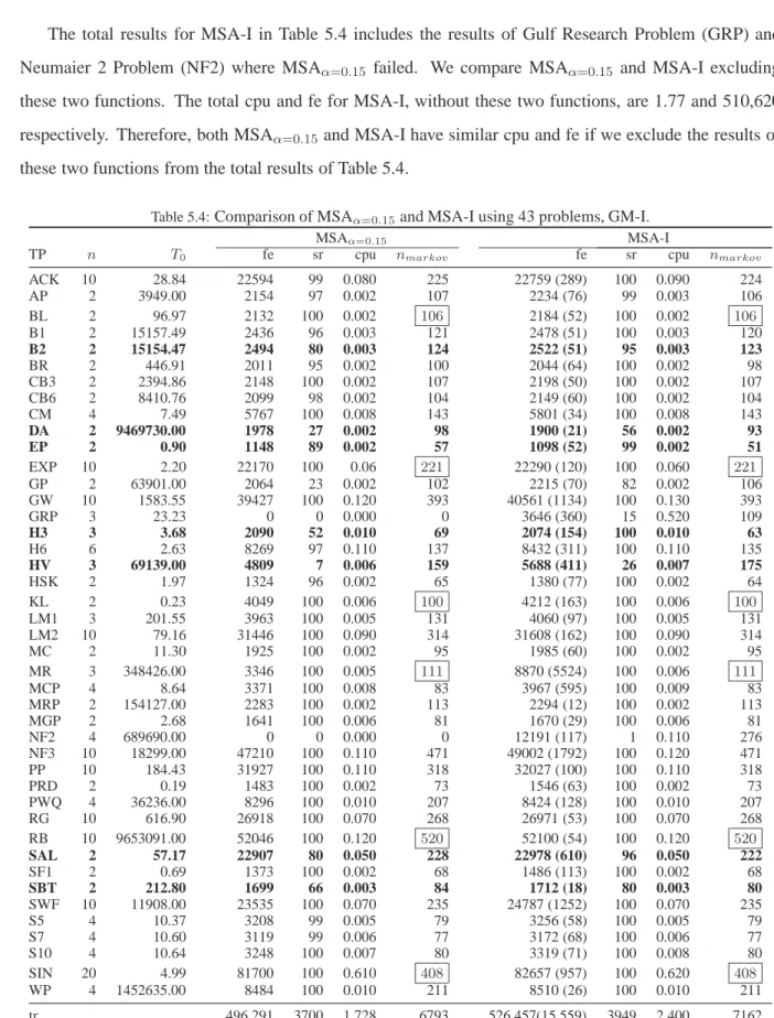
Simulated annealing driven pattern search algorithms for global optimization

(1)

Simulated Annealing Driven Pattern Search

Algorithms for Global Optimization

Musa Nur Gabere

School of Computational and Applied Mathematics

A dissertation submitted to the Faculty of Science,

University of the Witwatersrand, in fulfillment of the requirements for the degree of Master of Science.

(2)

Declaration

I declare that this dissertation is my own, unaided work. It is being submitted for the Degree of Master of Science to the University of the Witwatersrand, Johannesburg. It has not been submitted before for any degree or examination to any other University.

Musa Nur Gabere

(Date)

(3)

Abstract

This dissertation is concerned with the unconstrained global optimization of nonlinear problems. These problems are not easy to solve because of the multiplicity of local and global minima. In this dissertation, we first study the pattern search method for local optimization. We study the pattern search method numerically and provide a modification to it. In particular, we design a new pattern search method for local optimization. The new pattern search improves the efficiency and reliability of the original pattern search method. We then designed two simulated annealing algorithms for global optimization based on the basic features of pattern search. The new methods are therefore hybrid. The first hybrid method is the hybrid of simulated annealing and pattern search. This method is denoted by MSA. The second hybrid method is a combination of MSA and the multi-level single linkage method. This method is denoted by SAPS. The performance of MSA and SAPS are reported through extensive experiments on 50 test problems. Results indicate that the new hybrids are efficient and reliable.

Keywords: Global optimization, pattern search, simulated annealing, multi level single linkage, non-linear optimization, hybridization.

(4)

Dedication

Dedicated to my Mum

Marian Elmi Hassan

(5)

Acknowledgement

First and foremost, I give my appreciation to ALLAH (swt), the Cherisher and Sustainer of the Worlds for His Infinite Blessings and Guidance in my life.

I would like to express my sincere gratitude to my supervisor, Prof. Montaz Ali, who has put his enormous effort and time in the supervision of this dissertation. He has helped me to develop the research skills necessary to produce this document. I have relied on his knowledge of the field and guidance for implementing various algorithms. He also provided me with the neccessary tools for research such as routines for the test problems and simulated annealing. His innumerable and insightful suggestions have ultimately shaped this document. Without his help, this dissertation would not have realised.

I cannot miss to mention the love, support and devotion of my family. They have given me the strength and encouragement, that made me complete my studies. Many thanks goes to my Mum, Marian, my Dad, Nur, my one and only sister, Shugri and all my brothers, namely Mahammed, Abdi, Hassan, Abdihakin and Bashir. Special thanks goes to my elder brother, Mahammed, for his constant communication and encouragement.

Helpful email correspondence with Dr. Professor Kaelo is gratefully acknowledged. I also thank my colleagues who have helped me at every step of the way. Special thanks goes to Mihaja, Naval, Gasper, Morgan and Charles.

Lastly, my special gratitude goes to the School of Computational & Applied Mathematics and the African Institute for Mathematical Sciences (AIMS) for their financial support towards my research.

(6)

Nomenclature

Acronyms

PS Pattern search

MPS Modified pattern search SA Simulated annealing

MSA Modified simulated annealing

SAPS Simulated annealing driven pattern search MSL Multi level single linkage

Superscripts used throughout this dissertation k Iteration counter sa Simulated annealing t Temperature counter General symbols Ω Search region N Sample size

n Dimension of the problem f Objective function

x A vector

min/max Minimize/Maximize

xi Theithcomponent of the vectorx li Lower bound in theithdimension ui Upper bound in theithdimension

(7)

vi Symbols related to pattern search

x(k) kthiterate ofx.

∆k Step size parameter at iteratek

∇ First order derivative

D The set of positive spanning directions θk Expansion factor at iterationk

φk Contraction factor at iterationk

lim inf Limit inferior η Step factor

Symbols related to simulated annealing χ Acceptance ratio

kB Boltzmann’s constant m0 Number of trial points

m1 Number of successful trial points

m2 Number of unsuccessful trial points

δ Cooling rate control parameter εs Stop parameter

Ei Energy state of the system configurationi

∆Ei Difference in energy between new and current configurations p Probability

si State

Symbols related to MSA and SAPS hybrid RD Random direction

∆sa

0 Initial step size parameter used inside SA

xb The best point vector xρ_i Sample point

(8)

List of Figures

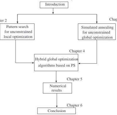
1.1 The structure of the dissertation. . . 6

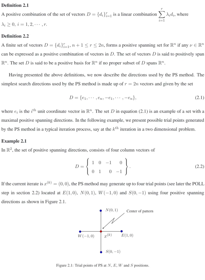
2.1 Trial points of PS atN,E,W andSpositions. . . 8

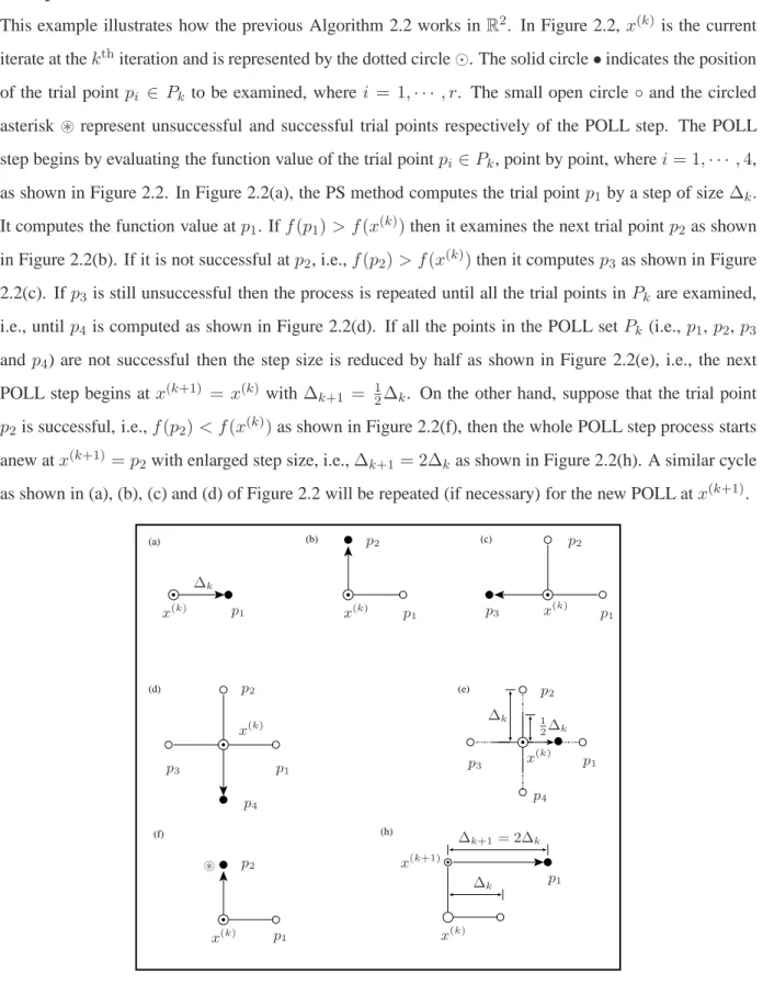
2.2 Figures (a)-(f) shows how the POLL steps works in the PS method. . . 13

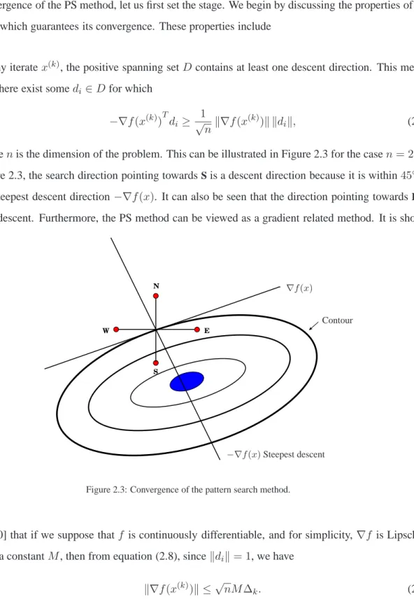
2.3 Convergence of the pattern search method. . . 14

2.4 The first trial point by MPS. . . 18

2.5 The generation of the second trial point by MPS when the first trial point is unsuccessful. 18 2.6 The generation of the second trial point of MPS when the first trial point is successful. . . 19

4.1 Flowchart for the MSA algorithm. . . 32

4.2 Flowchart for the SAPS algorithm. . . 36

5.1 Effect ofTton∆sa_t for HSK problem. . . 68

5.2 Effect ofTton∆sat for GP problem. . . 68

5.3 Effect ofTton∆sat for S5 problem. . . 69

5.4 Effect ofTton∆sa_t for RB problem. . . 69

5.5 Profile of∆c_t and∆sa_t for BP problem. . . 70

5.6 Profile of∆c_t and∆sa_t for KL problem. . . 71

(12)

List of Tables

5.1 Comparison of PS, PS-I and MPS using 32 problems. . . 42

5.2 Results of MSA for different values ofζ, GM-I. . . 45

5.3 Comparison of differentαvalues in MSA using 41 problems, GM-I. . . 46

5.4 Comparison of MSAα=0.15and MSA-I using 43 problems, GM-I. . . 48

5.5 Results of MSAα=0.15using 43 problems, GM-II. . . 50

5.6 Results of SAPS for different values ofδ, GM-I. . . 52

5.7 Results of SAPS for different values ofβ, GM-I. . . 54

5.8 Results of SAPS for different values ofβ, GM-I. . . 56

5.9 Results of SAPS forβ= 20using 43 problems, GM-II. . . 58

5.10 Results of SAPS for different sample sizeN, GM-I. . . 59

5.11 Results of SAPS usingN= 5n&γ= 1using 43 problems, GM-I.. . . 61

5.12 Results of SAPS usingN= 5n&γ= 0.5using 43 problems, GM-I.. . . 63

5.13 Results of SAPS usingN= 5n&γ= 0.25using 43 problems, GM-I. . . 65

5.14 Comparison of the algorithms using total results. . . 66

5.15 Rank order of algorithms. . . 67

B.1 Epistatic Michalewicz’s global optimizers. . . 78

B.2 Data for Hartman 3 problem. . . 79

(13)

LIST OF TABLES xii

B.5 Data for Kowalik problem. . . 81

B.6 Data for Meyer & Roth problem. . . 82

B.7 Data for modified Langerman problem. . . 82

B.8 Global optimizers for modified Langerman problem. . . 83

B.9 Data for Multi-Gaussian problem. . . 83

B.10 Global minima for Neumaier 3 problem. . . 84

B.11 Data for Price’s transistor modelling problem. . . 85

B.12 Global optimizers for Schubert problem. . . 87

B.13 Data for Shekel problem family. . . 88

B.14 Data for Shekel’s foxholes problem. . . 89

B.15 Global optimizers for Shekel’s foxholes problem. . . 89

(14)

Chapter 1

Introduction

Optimization is an important research area. It is the study of problems in which one seeks to minimize or maximize a real function by systematically choosing the values of real or integer variables within an al-lowed set. Optimization is mainly divided into two branches namely continuous and discrete optimization. A continuous optimization is where the variables used in the objective function assume real values. On the other hand, a discrete optimization is where the variables used in the objective function are restricted to as-sume only discrete values, such as integers. Continuous optimization problems can be classified according to the mathematical structure of the objective function and constraints. For example, a problem that has linear objective function and linear constraints is called a linear optimization problem. On the other hand, a problem that has nonlinear (linear) objective function with nonlinear or linear (nonlinear) constraints is called a nonlinear optimization problem. In other words, a nonlinear optimization problem is where the objective function or the constraints or both contain nonlinear terms. A nonlinear optimization problem can either be unconstrained or constrained depending on the presence of constraints or limitations on the variables.

A nonlinear optimization problem can have more than one optimal solution. The goal of a local op-timization method is to obtain any one of the optimal solutions. On the other hand, the goal of a global optimization method is to obtain the best optimal solution from a number of solutions. The best (global) optimal solution is not only hard to determine but also hard to verify. Despite its inherent difficulties, global optimization is vital to many practical applications. Some of these applications include, but not restricted to engineering design, financial risk management, computational chemistry, molecular biology and economics [8, 28]. Global optimization problems can be classified according to the properties of the

(15)

1.1 Problem formulation 2 objective function and constraints. A problem that has no constraints or constrained by simple lower and/or upper bounds is called unconstrained global optimization problem. A problem that has linear (nonlinear) constraints and nonlinear objective function is called a linearly (nonlinearly) constrained global optimiza-tion problem. These problems arise in real-life applicaoptimiza-tions. In many applicaoptimiza-tions, global optimizaoptimiza-tion problems are of black-box type. A black-box scenario occurs whenever the objective function and/or con-straints are not given in closed form, i.e., if the objective function values and/or concon-straints are evaluated via complex computations, simulations or experiments.

Our research is concerned with the design of unconstrained global optimization algorithms for solving both noisy and black-box type global optimization problems. An ideal global optimization algorithm should:

• work for a wide range of problems, be it easy, moderately difficult or difficult problems [47],

• not depend on the properties (e.g., continuity) of the objective function to be optimized,

• be easy to implement, and

• require very little computational effort.

It is not so easy to design an algorithm that satisfies all the above criteria. In any case, progress have been made and a number of global optimization algorithms have been suggested in the literature. We will review these algorithms later in the chapter. In the next section, we will present the global optimization problem mathematically.

1.1 Problem formulation

We consider the problem of finding the global optimum of box-constrained global optimization problems. The mathematical formulation of the global optimization problem is defined as follows

optimize f(x) subject to x_∈Ω, (1.1)

wherex= (x1,· · ·, xn)is ann−dimensional vector of unknowns,Ω⊆Rnis the search region, andf is

a nonlinear continuous real-valued objective function, i.e.,f : Ω _→R. The domain of the search space,

Ω, is defined by specifying an upper limituiand a lower limitli of eachithcomponent ofx, i.e.,

(16)

1.2 Classification of global optimization methods 3 Without loss of generality, we consider only the global minimization problem since the global maxi-mum can be found in the same way by reversing the sign off, i.e.,

max

x∈Ω f(x) =−minx∈Ω(−f(x) ). (1.3)

A point x∗ _∈ Ω is called a global minimizer of f with the corresponding global minimum value f∗=f(x∗)if

f∗_≤f(x), for all x_∈Ω. (1.4)

On the other hand, a pointxloc_∈Ωis referred to as a local minimizer offoverΩif there is anǫ >0such that

f(xloc)_≤f(x), for all x_∈Nǫ(xloc)∩Ω, (1.5) whereNǫ(xloc)

def

= _{x_∈Rn : _kx₋xloc_k< ǫ_}.

1.2 Classification of global optimization methods

Global optimization methods can be classified as deterministic and stochastic methods [22, 26]. Deter-ministic methods usually use gradient information and other properties such as known Lipschitz constant off. The main disadvantage of deterministic methods is that they cannot be implemented in noisy and black-box type functions. In addition, these methods are very slow as they often perform an exhaus-tive search. As opposed to deterministic methods, stochastic methods are very easy to implement and in most instances, they do not require any functional properties. Hence these methods are widely applicable. Unlike deterministic methods, which guarantee convergence to the global minimum, stochastic methods assures convergence in a probabilistic sense. In addition, the computational costs of stochastic methods are in general less than those of deterministic methods [41]. For this reason, in this dissertation, we con-centrate on stochastic methods, in particular simulated annealing and multi level single linkage with some hybridization. We will briefly present some deterministic and stochastic methods.

One of the best known deterministic method is the interval arithmetic method [27] for global opti-mization. It is based on the branch-and-bound method [38]. The branch-and-bound method is a technique where the feasible region is relaxed and subsequently split into parts (branching) over which the lower (and often also the upper) bounds of the objective function value can be determined (bounding). Another important deterministic method is the multi-dimensional bisection method [52] which is a generalization of the bisection method [16] to higher dimensions. It begins by generating a sequence of intervals whose

(17)

1.2 Classification of global optimization methods 4 infinite intersection is the set of points desired. However, unlike interval arithmetic method, this method never attracted the global optimization researchers and practitioners. In addition to the above determin-istic methods, Breiman and Cutler [18] designed a determindetermin-istic algorithm for global optimization. This algorithm assumes a bound on the second derivatives of the function and uses this to construct an upper envelope. Successive function evaluations lower this envelope until the value of the global minimum is found. Other deterministic methods include αBB [1], Lipschitz method, methods based on convex en-velopes of the objective function over special domain like boxes. There are softwares developed to solve deterministic global optimization. Currently the branch-and-reduce optimization navigator (BARON) [43] is the best software in the field of deterministic global optimization.

Stochastic methods are either single sample (point) based or multiple sample (population) based meth-ods. Within the single sample based methods, tabu search [19], adaptive random search [35] and simulated annealing [2, 21] are well known. Among the population based methods, density clustering [41], multi level single linkage [42] and topographical multilevel single linkage [13] often referred to as two-phase methods. Two-phase methods use both random sampling (global phase) and local search (local phase). In the global phase, the function is evaluated in a number of randomly sampled points while in the local phase, the sample points are scrutinised by a clustering technique in order to identify potential points to start a local search. A more detailed survey of the two-phase methods for stochastic global optimization can be found in [44].

Other population based methods are genetic algorithm [23], controlled random search [6, 10, 40] and differential evolution [12, 45]. These methods start with an initial population set of points, drawn uniformly in the search space Ω and subsequently manipulating this sample in order to obtain a better population set. The better population set is obtained by replacing all or some members of the current set with new trial points. The mechanism used in creating trial points depends on the considered algorithm [11]. For example, in genetic algorithm, trial points are generated by selecting successively a subset of the population and then applying mutation and crossover operations on this set. In controlled random search, a trial point is generated by forming a simplex using(n+ 1)distinct points, chosen at random with replacement from the population set, and reflecting one of the points in the centroid of the remainingn points of the simplex, as in the Nelder and Mead algorithm [37]. In differential evolution, trial points are generated using mutation and crossover operations. In addition to the above stochastic methods, there exist hybrid methods. The purpose of hybrid methods is to use the complementary strengths of several methods within a single method. Next, we present the main features of the hybrid method for global optimization.

(18)

1.3 Hybridization 5

1.3 Hybridization

Hybridization is basically the combination of principles (elements) from different methods so as to give rise to a new method that displays desirable properties of the original methods but not their weaknesses.

There are different ways to hybridize methods which combine two methods [39, 46]. One approach is to run one algorithm until it stops before the next one is started. This is known as sequential hybridiza-tion. Another approach is to run the algorithms in parallel in a pre-defined manner, e.g., the next method starts before the previous one ends. This is known as parallel hybridization. However, in most cases, hy-bridization is achieved by combining algorithmic elements of the original methods to end up with a single algorithmic architecture. For instance, a popular approach is to combine global features of a global method with local features of a local method. Local methods are computationally efficient because they make use of local information around the current point to move to a promising region. This expedites convergence whenever a point is within the region of attraction of a minimum. On the other hand, global methods are more reliable in locating the global minima because they explore the whole search region and have mechanisms to escape being trapped in local minima. Consequently they are computationally expensive.

It is expected that the combination of elements from local methods with those of global methods would result in methods that are more efficient, more accurate and more reliable in finding the global minimum. Efficiency refers to the amount of efforts (be it CPU time or number of function evaluations) required to obtain a solution. Accuracy means how close is the final solution obtained by a global optimization algorithm to the known global minimum of a problem. Reliability is how successful is the method in finding the global minimum. Hence such hybrid methods would result into being more reliable in locating the global minimum than a local method and also more accurate and more efficient than a global method. Examples of hybrid methods include but not restricted to simulated annealing combined with direct search hybrid [9, 31] and tabu search combined with Nelder-Mead simplex hybrid [20].

We aim at designing hybrid methods that will possess only strengths of the original methods. In this dissertation, we will combine global methods (simulated annealing, multi level single linkage) and a local method (pattern search).

(19)

1.4 The structure of the dissertation 6

1.4 The structure of the dissertation

The dissertation is divided into six chapters as shown in Figure 1.1. In Chapter 2, we address the strengths and weaknesses of the pattern search method. We first review the pattern search method in relation to its description, convergence properties and its limitations in solving global optimization problems. Then we propose a modified pattern search method.

In Chapter 3, we present an overview of the simulated annealing method in regard to its origin. We also present the simulated annealing for continuous problems and the cooling schedule.

In Chapter 4, we propose two new hybrid methods based on the pattern search method, the simulated annealing method and the multi level single linkage method.

In Chapter 5, we report the performance of the proposed hybrid methods using extensive numerical experiments on some well known test problems.

In Chapter 6, we summarize the work in this dissertation and propose further avenues to extend and enhance this research. Finally, we give a description of the multi level single linkage algorithm and a collection of 50 benchmark global optimization test problems in Appendixes A and B, respectively.

Introduction Pattern search for unconstrained local optimization Simulated annealing for unconstrained global optimization

Hybrid global optimization algorithms based on PS Numerical results Conclusion Chapter 1 Chapter 2 Chapter 3 Chapter 4 Chapter 5 Chapter 6

(20)

Chapter 2

Pattern search for unconstrained local

optimization

The pattern search method [30, 48] is a recent direct search method for local optimization. In this chapter, we describe the pattern search method for unconstrained local optimization and propose a modification to it.

2.1 The pattern search (PS) method

In its simplest form, the PS method is a variation of the coordinate search method [30]. However, the mathematical formalization presented by Torczon [48] shows that the PS method is a general class of the direct search methods. For instance, the Hooke and Jeeves method [25], the basic coordinate search method [30] and the multi-directional search method [49] also form part of the PS method. As such, in some literature [15], the PS method is referred to as the generalized pattern search (GPS) method. In this dissertation, we only deal with a simple but effective variant of the PS method. Before we describe the PS method, we give two definitions [4] that are essential for understanding the search directions of this method. We also present an example of the search directions used by the PS method in a typical two dimensional problem.

(21)

2.1 The pattern search (PS) method 8 Definition 2.1

A positive combination of the set of vectorsD=_{di}ri=1is a linear combination

r X i=1 λidi, where λi≥0, i= 1,2,· · · , r. Definition 2.2

A finite set of vectorsD=_{di}ri=1,n+ 1≤r ≤2n, forms a positive spanning set forRnif anyν∈Rn

can be expressed as a positive combination of vectors inD. The set of vectorsDis said to positively span Rn. The setDis said to be a positive basis forRnif no proper subset ofDspansRn.

Having presented the above definitions, we now describe the directions used by the PS method. The simplest search directions used by the PS method is made up ofr= 2nvectors and given by the set

D=_{e1,· · ·, en,−e1,· · ·,−en}, (2.1) whereeiis theithunit coordinate vector inRn. The setDin equation (2.1) is an example of a set with a maximal positive spanning directions. In the following example, we present possible trial points generated by the PS method in a typical iteration process, say at thekthiteration in a two dimensional problem. Example 2.1

InR2, the set of positive spanning directions, consists of four column vectors of

D=    1 0 ₋1 0 0 1 0 ₋1    . (2.2)

If the current iterate isx(k)_{= (0}_,₀₎_{, the PS method may generate up to four trial points (see later the POLL}

step in section 2.2) located at E(1,0), N(0,1), W(₋1,0) and S(0,₋1) using four positive spanning directions as shown in Figure 2.1.

E(1,0) Center of pattern N(0,1) W(−1,0) S(0,−1) x(k)

(22)

2.2 Description of the PS method 9

2.2 Description of the PS method

In this section, we present a full description of the PS method. The PS method generates a sequence of iterates {x(1)_{, x}(2)_,_{· · ·}_x(k)_,_{· · · }}_{with non-increasing objective function values. In each iteration}_{k, there}

are two important steps of the PS method namely, the SEARCH step and the POLL step. Note that we use the valuer = 2nin the description of the PS method.

In the SEARCH step, the objective function is evaluated at a finite number of points (say a maximum ofV _{points) on a mesh (a discrete subset of} _Rn₎ _{so as to improve the current iterate. The mesh at the} current iterate,x(k), is given by

Mk={m∈Rn|m=x(k)+ ∆kDq : q ∈Zr+}, (2.3)

where m is a mesh trial point, ∆k > 0 is a mesh size parameter (also known as the step size control parameter) which depends on the iteration k, and Z+ is the set of nonnegative integers. There are no

specific rules on how to generate trial points of the SEARCH step in the current mesh. Users may generate these points by some heuristic rules. The aim of the SEARCH step is to find a feasible trial point (on a mesh Mk) that yields a lower objective function value than the function value at x(k). A SEARCH step is therefore successful if there exists a feasible trial pointm_∈Mk(wheremis one of theVpoints) such that f(m) < f(x(k)). In such a case, mis treated as the new iterate and the step size ∆k is increased so as to choose the next trial points on a magnified mesh than the previous mesh. If the SEARCH step is unsuccessful in improving the current iteratex(k), a second step, called the POLL step, is executed around x(k) _{with the aim of decreasing the objective function value. This step must be done before terminating}

the iteration.

The POLL step generates trial points at the poll set around the current iterate,x(k)_{, as shown in Figure}

2.1, for the case of a two dimensional problem, where∆k= 1. The poll set is composed of trial points that are positioned a step∆kaway from the current iteratex(k), along the direction designated by the columns ofD. This poll set is denoted byPkand is defined by

Pk={pi ∈Rn|pi =x(k)+ ∆kdi : di ∈D, i:= 1,· · · , r}, (2.4) wherepiis a trial point in the POLL step. The order in which the points inPkare evaluated can also differ and has no effect on convergence. We now present the step by step description of the PS algorithm [3] using both the SEARCH and the POLL step.

(23)

2.2 Description of the PS method 10

Algorithm 2.1: The PS algorithm (based on the SEARCH and the POLL steps).

1. Initialization: Choose an initial pointx(0) _∈ _Ω_{and an initial mesh size}_∆

0 > 0. Set the iteration

counterk= 0.

2. SEARCH step:. Evaluate f at a finite number of points in the meshMk as defined by (2.3). If f(m) < f(x(k)₎ _{for some}_m _∈ _M

kthen set x(k+1) = m and go to step4 (the SEARCH step is deemed successful). If the SEARCH step is unsuccessful, i.e.,f(x(k)) _≤f(m), for allV_{points in} Mkthen go to step 3.

3. POLL step: This step is executed only if the SEARCH step is unsuccessful.

• Iff(pi)< f(x(k))for somepiin the poll setPkdefined by (2.4), then setx(k+1) =piand go to step4in order to increase the mesh size∆k, (POLL step is declared successful).

• Otherwise iff(x(k)₎_≤_f₍_p

i)for allpi in the poll setPkdefined by (2.4) , setx(k+1) =x(k) and go to step5in order to decrease the mesh size∆k, (POLL step is declared unsuccessful). 4. Mesh expansion: Let∆k+1=θk∆k, (withθk>1). Increasek:=k+ 1and go to step2for a new

iteration.

5. Mesh reduction: Let∆k+1 =φk∆k, (with0< φk<1). Increasek:=k+ 1and go to step2for a new iteration.

In summary, Algorithm2.1performs the SEARCH and the POLL step. In the SEARCH step, the objective functionf is evaluated at a finite number of trial pointsm _∈ Mkwith the goal of improving the current iteratex(k). If an improvement is accomplished, then the trial pointmbecomes the current iterate and the mesh size is increased, i.e.,∆k+1 =θk∆kand the SEARCH step continues. Otherwise, if the SEARCH step is unsuccessful in improving the current iterate x(k), for all V_{, a second step called the POLL step} is invoked. If the POLL step is successful, i.e.,f(pi) < f(x(k))for some pi _∈ Pk thenpi becomes the new iterate, the mesh size is increased and the SEARCH step process is invoked. Iff(pi) ≥f(x(k))for allpi ∈ Pk then the current iteratex(k) is retained, the mesh size is decreased and the SEARCH step is performed.

(24)

2.2 Description of the PS method 11 In the literature of the PS method, no specific information is given on how to implement the SEARCH step. Indeed, the results of the PS method using only the POLL step are reported in the literature [3, 30]. It is also reported in [15] that the SEARCH step is a liability to convergence. Therefore, in this dissertation, we will only implement the POLL step in the PS method. Before we present the PS algorithm based on the POLL step, we would like to elaborate more on the POLL step. We discuss how the current iterate and the step size are updated in the POLL step.

The POLL step begins by determining a trial pointpiin the poll setPkdefined earlier, i.e.,

{pi ∈Rn|pi =x(k)+ ∆kdi : di ∈D, where i:= 1,· · · , r}, wherex(k)_{is the current iterate. The trial point}_p

iis examined so as to determine if it is a better solution than the current iterate x(k). (Here the trial point pi could be one of the positions, say for i = 1, it is E(1,0)of Figure 2.1). If the POLL step produces a successful pointpi ∈Pksuch thatf(pi) < f(x(k)), then the POLL step stops examining the remaining trial points in the current POLL setPk. This means that if the POLL step is declared successful then a new POLL step starts at this new current iteratex(k+1)₌_p

i. Otherwise, the current iterate is retained, i.e.,x(k+1) =x(k), whenf(pi)≥f(x(k))for all the trial points pi ∈ Pk, i.e., the POLL step is declared unsuccessful. Thus, the next iterate for the next POLL step is updated as follows: x(k+1)=      pi iff(pi)< f(x(k)),for somepi_∈Pk, x(k) otherwise. (2.5)

In the case of a successful POLL step, the step size parameter∆k+1for the next iteration is increased to

∆k+1=θk∆k, whereθk>1, in a similar fashion as in mesh expansion of Algorithm2.1. This enhances exploration of the PS method. However, when the POLL step is unsuccessful, then step size parameter is decreased to∆k+1 =φk∆k, for0< φk <1, in a similar way as in the mesh reduction of Algorithm2.1. This in turn enhances exploitation. In summary the step size parameter is updated [48] as follows:

∆k+1=      θk∆k iff(pi)< f(x(k)),for somepi∈Pk, φk∆k otherwise. (2.6)

This POLL step is reiterated until the step size parameter∆kgets sufficiently small, thus ensuring conver-gence to a local minimum. Note that asx(k)approaches the optimum, the algorithm reduces the length of steps taken. This turns out to be central to the convergence proof which will be discussed in section 2.3.

(25)

2.2 Description of the PS method 12 In most implementation of the PS method, the initial step size parameter ∆0 = 1 is used and the

updating of the step size parameter is carried out by

∆k+1 =      2∆k iff(pi)< f(x(k)),for somepi ∈Pk, θk= 2, 1 2∆k otherwise, φk= 12. (2.7)

The basic PS method based only on the POLL step described above is presented in Algorithm2.2below. Note that from now on, the PS algorithm based on the POLL step will be referred to as the PS algorithm.

Algorithm 2.2: The PS algorithm.

1. Initialization:

Choose an initial feasible solutionx(0) _∈_Ω_{. Select an initial step size}_∆

0 >0. Choose the positive

spanning setDdefined by equation (2.1). Set the counter numbersk = 0and i = 1. Choose the stopping tolerance∆tol >0.

2. POLL step:

2(a) Evaluate the objective functionf at the trial pointpi = (x(k)+ ∆kdi)∈Pk,di∈D. 2(b) Iff(pi)< f(x(k))then setx(k+1) =pi and go to step 3.

Otherwise, increasei:=i+ 1and go to step 2(c). 2(c) Ifi_≤rthen go to step 2(a).

Otherwise, setx(k+1) =x(k)and go to step 4.

3. Mesh expansion: Increase the step size parameter∆k+1 =θk∆k. Seti= 1and go to step 5. 4. Mesh reduction: Decrease the step size parameter∆k+1=φk∆k. Seti= 1and go to step 5. 5. Stopping condition: If∆k+1<∆tol then stop. Otherwise, increasek:=k+ 1and go to step 2.

Having described the PS algorithm, we now illustrate a step by step process of this algorithm, using the following example. In this example. we useθk = 2andφk= 1₂.

(26)

2.2 Description of the PS method 13 Example 2.2

This example illustrates how the previous Algorithm 2.2 works inR2. In Figure 2.2, x(k) is the current iterate at thekth_{iteration and is represented by the dotted circle}_⊙_{. The solid circle}_•_{indicates the position}

of the trial pointpi ∈ Pk to be examined, wherei = 1,· · ·, r. The small open circle◦ and the circled asterisk⊛represent unsuccessful and successful trial points respectively of the POLL step. The POLL step begins by evaluating the function value of the trial pointpi∈Pk, point by point, wherei= 1,· · · ,4, as shown in Figure 2.2. In Figure 2.2(a), the PS method computes the trial pointp1by a step of size∆k. It computes the function value atp1. Iff(p1)> f(x(k))then it examines the next trial pointp2as shown

in Figure 2.2(b). If it is not successful atp2, i.e.,f(p2)> f(x(k))then it computesp3as shown in Figure

2.2(c). Ifp3 is still unsuccessful then the process is repeated until all the trial points inPkare examined, i.e., untilp4 is computed as shown in Figure 2.2(d). If all the points in the POLL setPk(i.e., p1,p2,p3

and p4) are not successful then the step size is reduced by half as shown in Figure 2.2(e), i.e., the next

POLL step begins atx(k+1) ₌ _x(k) _with_∆

k+1 = 1₂∆k. On the other hand, suppose that the trial point p2 is successful, i.e.,f(p2) < f(x(k))as shown in Figure 2.2(f), then the whole POLL step process starts

anew atx(k+1) ₌_p

2with enlarged step size, i.e.,∆k+1= 2∆kas shown in Figure 2.2(h). A similar cycle as shown in (a), (b), (c) and (d) of Figure 2.2 will be repeated (if necessary) for the new POLL atx(k+1).

(a) (b) (c) (d) (e) (h) (f) x(k) x(k) p1 p1 p1 x(k) _x(k) x(k) x(k) x(k) ∆k ∆k 1 2∆k p1 p1 p1 p1 p2 p2 p2 p2 p2 p3 p3 p3 p4 p4 ∆k ∆k+1= 2∆k ⊛ x(k+1)

(27)

2.3 The convergence properties of the PS method 14

2.3 The convergence properties of the PS method

In this section, we will discuss the convergence of the PS method. Before proceeding to a formal statement of the convergence of the PS method, let us first set the stage. We begin by discussing the properties of the PS method which guarantees its convergence. These properties include

1. At any iteratex(k), the positive spanning setDcontains at least one descent direction. This means that there exist somedi ∈Dfor which

−∇f(x(k))Tdi≥ 1 √ nk∇f(x (k)₎ k kdik, (2.8)

wherenis the dimension of the problem. This can be illustrated in Figure 2.3 for the casen= 2. In Figure 2.3, the search direction pointing towardsSis a descent direction because it is within45◦ _of

the steepest descent direction_−∇f(x). It can also be seen that the direction pointing towardsEis also descent. Furthermore, the PS method can be viewed as a gradient related method. It is shown

S E N W ∇f(x) −∇f(x)Steepest descent Contour

Figure 2.3: Convergence of the pattern search method.

in [30] that if we suppose thatf is continuously differentiable, and for simplicity,_∇f is Lipschitz with a constantM, then from equation (2.8), since_kdi_k= 1, we have

(28)

2.4 Pros and cons of the PS method 15 2. Ask_→ +_∞, the total number of successful iterations must be finite. This means that the number

of unsuccessful iterations (in POLL) is infinite. Therefore,∆k→0ask→+∞.

Clearly, the convergence analysis of the PS method is based on the standard assumption that all trial points produced by the algorithm lie in a compact set. That is, the level set_{x_∈Ω :f(x)< f(x(0)₎_}_is

bounded. This boundedness of the level set will ensure that the step size parameter satisfies

lim

k→+∞∆k= 0. (2.10)

It has been established in [48] that the PS method possesses the convergence property i.e.

lim inf

k→+∞k∇f(x

(k)₎

k= 0, (2.11)

which follows directly from equation (2.9) and equation (2.10).

After discussing the convergence of the PS method, we now focus our attention in elaborating some of the pros and cons of the PS method with regard to solving global optimization problems. We briefly discuss the pros and cons of the PS method and thereafter propose a modification that will eliminate some of its limitations.

2.4 Pros and cons of the PS method

Associated with the PS method are the following advantages :

• It is a direct search method and does not depend on any properties (continuity or differentiability) of the objective function being optimized.

• It initially makes a rapid progress towards a local solution, i.e., excellent convergence characteristics.

• It is easily programmable and easy to implement.

We studied the numerical efficiency and robustness of the PS method. We applied the PS method on50

simple bounded global optimization test problems (see Appendix B). Our numerical experiments suggested the following shortcomings of the PS method.

1. The initial step size parameter∆0. Another problem experienced by the PS method is its

(29)

2.5 The modified pattern search method 16 large search regions and hence takes longer time to converge. Also it is not appropriate for problems with small search regions.

2. Badly scaled function. The PS method is very slow to converge when the level sets of the function are extremely elongated. This is because of its use of coordinate directions.

3. Dimensionality problem. Lastly, the PS method suffers from curse of dimensionality. As the number of dimension increases, the PS method breaks down.

Having discussed the limitations, we aim at remedying some of these limitations of the PS method.

2.5 The modified pattern search method

In this section we will discuss how to eliminate some of the shortcomings of the PS method. Among the shortcomings of the PS method, the initial step size ∆0 and searching along coordinate directions were

very sensitive. Hence we suggest the following modifications.

To deal with the problem of initial step size parameter (∆0 = 1), we decided to use an initial step size

parameter which depends on the size of the search regionΩ. We propose

∆0 = max{ui−li|i= 1,· · · , n}/2, (2.12) where ui and li are upper and lower bounds respectively of the search region Ω for each dimension. The initial stepsize∆0 = 1used in PS for unconstrained local optimization where no bounds exists for the

variable of the problem. The property∆k→0ask→ ∞is an important ingredient for the convergence of PS. In this study, we used∆0in equation (2.12) to solve bound constrained global optimization problems.

The step size∆0is used in such a way that it takes into account on the size of the search space. There are

instances whereby the componentpj_i > uj (orpji < uj) of the trial pointpi = (p1i,· · · , pni)falls outside

Ω. In these cases, we re-generate a trial pointpiwith the component

pj_i =x(k)j +ω(uj −x(k)j), or

pj_i =lj+ω(x(k)j−lj),

(30)

2.5 The modified pattern search method 17 To deal with the problem of searching along coordinate direction, we decided to use a perturbation of the coordinate direction. This modification is described as follows. Starting at the current iterate x(k)at thekth_{iteration, the POLL step computes the next iterate}_p

i∈Pkby a step size∆kin the same way as in the PS method. However, it does not compute the function value atpias in the PS method. Instead it uses this point as a stepping stone to compute the trial pointp˜iwith a step of sizer =η∆kand this trial point

˜

piis given by

˜

pi=pi+r×U, (2.13)

whereU = (U1, . . . , Un)T is a directional cosines with random components

Uj =Rj/(R21+· · ·+R2n)

1/2

, j= 1,_{· · ·} , n, (2.14) Rj is a uniform random number in the interval[−1,1]. The PS method equipped with (2.12) and (2.13) is denoted by MPS. The above modifications in equation (2.12)-(2.14) preserves the convergence properties of the PS method. The POLL step of this modification can be explained using the following example. Example 2.3

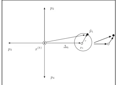
The POLL step of this modification is explained as follows using Figures 2.4, 2.5 and 2.6. In these Figures, the definitions of the dotted circle _⊙, solid circle _•and⊛are the same as in example2.2 except for the small open circle◦which represents a stepping point. Given the current iteratex(k)_{in Figure 2.4, the point}

p1is first computed as in POLL step of Algorithm 2.2. Unlike the PS method, the MPS does not calculate

the function value at p1. In its place, a new neighboring point p˜1 using equation (2.13) is calculated

uniformly on the surface of a hypersphere with radius r. The POLL step then compares the function values off(x(k)₎_and _f_(˜_p

1). If it is successful, i.e.,f(˜p1) < f(x(k))then the new POLL step begins at

the new iteratex(k+1) = ˜p1with∆k+1= 2∆kas in the POLL step of Algorithm2.2. If it is unsuccessful, i.e.,f(˜p1) ≤f(x(k))then the second coordinate direction is used indirectly to generate the trial pointp˜2

as shown in Figure 2.5. This process is reiterated. If none of the trial points,p˜i, (fori= 1,· · · , r), is better than the current iteratex(k)_{then the POLL step begins at}_x(k+1) ₌_x(k)_with_∆

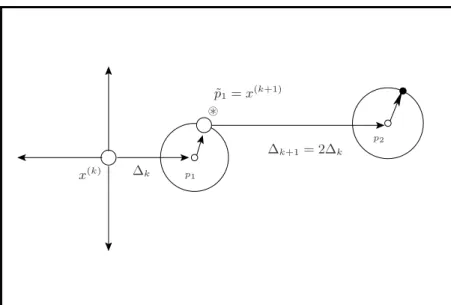
k+1 = ∆k/2. Figure 2.6 shows that the pointp˜1is successful and the new POLL step begins atx(k+1)= ˜p1with∆k+1= 2∆k.

(31)

2.5 The modified pattern search method 18 x(k) ∆k r p₁ ˜ p1 p2 p3 p4

Figure 2.4: The first trial point by MPS.

x(k) p1 p₂ ˜ p2 p3 p4 ∆k

(32)

2.6 Summary 19 ∆k ∆k+1= 2∆k x(k) _p 1 ˜ p1=x(k+1) p₂ ⊛

Figure 2.6: The generation of the second trial point of MPS when the first trial point is successful.

2.6 Summary

In this chapter, we have reviewed the PS method. The two main ingredient of the PS method, i.e., the SEARCH and the POLL step were discussed. Thereafter, we give a motivation as to why we discarded the SEARCH step in the PS algorithm. Furthermore, this chapter also elucidates the convergence properties of the PS method. The shortcomings of the PS method are elaborated and some strategies to deal with these shortcomings were suggested. The remaining limitation of PS, i.e., getting trapped in local minimum, will be ameliorated by hybridizing PS with simulated annealing with or without multi level single linkage.

(33)

Chapter 3

Simulated annealing for unconstrained

global optimization

This chapter forms the core of the hybrid methods that will be designed in Chapter 4. We review the physical annealing and the Metropolis algorithm [36]. We discuss the simulated annealing method [21] for continuous problems. Finally, we present the cooling schedule.

3.1 The physical annealing

The physical annealing is a thermal process for obtaining low energy states of a solid in a heat bath. At first, the solid is heated until all atoms are randomly arranged in a liquid state and then it is cooled by gradually lowering the temperature.

Central to physical annealing is the attainment of the thermal equilibrium. At each temperature, enough time is spent for the solid to reach the thermal equilibrium. If the liquid is cooled slowly enough, then crystals will be formed and the system will have reached its minimum energy at the ground state. However, if the system is cooled quickly, then it will end up in a polycrystalline or amorphous state (local optimal structure), i.e., trapped in a local minimum energy.

Computer simulation of the thermal equilibrium of a collection of atoms at a given temperature was achieved by Metropolis et al. [36]. They suggested an algorithm for obtaining the thermal equilibrium. The algorithm is known as the Metropolis algorithm. The genesis of the simulated annealing method is

(34)

3.2 The Metropolis procedure 21 based on principles of the condensed matter physics, in particular the physical annealing.

3.2 The Metropolis procedure

In1953, Metropolis et al. [36] used the Monte Carlo method, now known as the Metropolis algorithm, to simulate the collection of particles in thermal equilibrium at a given temperature T. The Metropolis algorithm generates a sequence of states of the system of particles or atoms in the following way. Given a current state,si, of the system of particles with corresponding energyEi, the system is perturbed to a new statesj with energyEj. If the change,∆E = Ej −Ei, represents a reduction in the energy value then the new statesj is accepted. If the change∆E represents an increase in the energy value, then the new state is accepted with probabilityexp(₋(∆E/kBT), whereT is the surrounding temperature andkB is the Boltzmann constant. The acceptance rule described above is called the Metropolis criterion and the algorithm that goes with it, is known as the Metropolis algorithm. The Metropolis algorithm is described as follows:

Algorithm 3.2: The Metropolis Algorithm. set surrounding temperatureT.

pick initial statesiat random. repeat

propose new statesjpicked at random;

∆E=Ej−Ei;

if∆E_≤0thenp= 1elsep= exp(₋∆E/kBT); if random[0,1)< pthensi =sj ;

until thermal equilibrium reached.

In the physical annealing, a thermal equilibrium is reached at each temperature if the lowering of the temperature is done sufficiently slowly. Similarly, in the case of the Metropolis algorithm, a thermal equilibrium can be achieved by generating a large number of transitions at a given temperature. At thermal equilibrium, the probability that the system of particles is in state, si, with energy Ei is given by the Boltzmann distribution, i.e.,

PT{X=si}= 1 Z(T) exp −E_i kBT , (3.1)

(35)

3.3 The simulated annealing (SA) method 22 whereXis a random variable denoting the current state of the system of particles andZ(T)is defined as

Z(T) =X j exp−Ej kBT . (3.2)

3.3 The simulated annealing (SA) method

In1983, Kirkpatrick et al. [29] designed the simulated annealing algorithm for optimization problems by simulating the physical annealing process. The formulation of the optimization algorithm using the above analogy consists of a series of Metropolis chains used at different values of decreasing temperatures. In this formulation, the system state corresponds to the feasible solution, the energy of the state corresponds to the objective function to be optimized, and the ground state corresponds to the global minimizer.

The general SA consists of two loops. In the inner loop, a number of points in a Markov chain (a Markov chain is a sequence of trial solutions) in the configuration space is produced and some of them are accepted. A trial solution is accepted only if it satisfies the Metropolis criterion. On the other hand, in the outer loop, the temperature is progressively decreased. The whole process depends on the cooling schedule which will be discussed in section 3.5. The original SA algorithm was intended for discrete optimization problem. The general description of the SA algorithm is as follows:

Algorithm 3.3: A general description of the simulated annealing algorithm. Generate the initial configurationsi.

Select an initial temperatureT =T0. while stopping criterion is not satisfied do begin.

while no complete Markov chain do begin

generate movesj; computef(sj);

if accept then update solutionsiandf(si); end;

decreaseT; end.

(36)

3.4 The simulated annealing algorithm for continuous problems 23

3.4 The simulated annealing algorithm for continuous problems

In this section, we present the SA algorithm for continuous optimization problems. The statessi and sj are now denoted by the pointsxandyrespectively inΩ. The corresponding energies of these states, i.e., EiandEj are therefore denoted by the function valuesf(x)andf(y)respectively.

The SA algorithm has been applied to optimization of multimodal continuous functions by fewer au-thors (Vanderbilt and Louie [50], Alluffi-Pentini et al. [14], Bohachevsky et al. [17] and Wang and Chen [51]) than for the optimization of discrete functions. However, firstly these methods are to some extent dif-ferent from the original SA approach to discrete optimization. Secondly, their theoretical convergence and sufficient numerical evidences on classified test problems justifying their reliability are missing. Dekkers and Aarts [21] derived a local search-based continuous simulated annealing (LSA) algorithm which is the-oretical similar to discrete SA. An aspiration-based simulated annealing (ASA) algorithm [7] and a direct search simulated annealing (DSA) algorithm [9] have also been developed which retains the convergence properties of LSA.

One of the complications arising in going from the discrete to the continuous application of SA is that of the point generation, i.e., generating a new pointyfrom a given point x. One of the possibilities is to generateyusing a uniform distribution on Ω; the generation probability distribution functiongxy, in this case, is given bygxy = 1/m(Ω)wherem(Ω)is the Lebesgue measure of the setΩ. However, this choice does not consider the structural information of function values and hence Dekkers and Aarts [21] put forward a mechanism consisting of two possibilities; either a point is drawn uniformly in the search region

Ωwith probabilityψ; or a step is made into a descent direction from the current pointxwith probability (1₋ψ), whereψis a fixed number in[0,1). Dekkers and Aarts [21] denote this generation mechanism by

gxy =      1 m(Ω) if ω ≤ψ, LS(x) if ω > ψ, (3.3)

whereω a uniform random number in[0,1). LS(x)denotes a local technique procedure that generates a pointyin a descent direction from xsuch thatf(y) _≤f(x). The local technique LS(x)fromxis not a complete local technique but only a few steps of some appropriate descent search. Thus, iff(y) < f(x)

thenyis not necessarily a local minimum.

Like any other standard SA algorithm based on Markov chains, the essential features of LSA, ASA and DSA are as follows: Starting from a randomly generated initial point x _∈ Ωand with an assigned

(37)

3.4 The simulated annealing algorithm for continuous problems 24 valueTt of the temperature parameter (the temperature countertis initially set to zero). These methods generates a new trial point,y, using the mechanism (3.3). The objective functionf(y)is calculated. If the change∆fxy = f(x)−f(y)represents a reduction in the value of the objective function then the new pointyis accepted. If the change represents an increase in the objective function value then the new point yis accepted using a Metropolis acceptance probability

Axy(Tt) = min{1,exp(−(f(x)−f(y) )/Tt)}. (3.4) This process is repeated for a large enough number of iterations for eachTt. A new Markov chain is then generated (starting from the last accepted point in the previous Markov chain) for a reduced temperature until the algorithm stops. The algorithm for continuous LSA [21] is sketched below.

Algorithm 3.4: The LSA algorithm for the continuous problem.

begin

initialize (T0, x);

stop criterion := false;

while stop criterion = false do begin

fori:= 1 toLdo begin

generateyfromxusing (3.3); iff(y)₋f(x)_≤0then accept;

else ifexp(₋(f(y)₋f(x) )/Tt)>random[0,1)then accept; if accept thenx:=y; end; lowerTt; end; end. Remark 3.1:

(38)

3.5 Cooling schedule 25 ofTt, and the stop criterion. All these are specified by the cooling schedule which is discussed in the next section

3.5 Cooling schedule

The choice of the cooling schedule (also known as the annealing schedule) is the heart of SA. The cooling schedule affects the number of times the temperature is decreased. We saw earlier in section 3.1 that if a system is cooled hastily, then it will end up with a polycrystalline state, i.e., a system with high energy. Similarly, in the case of an optimization problem, if a fast cooling takes place (i.e., temperature is decreased at a fast rate) then the problem will be trapped in a local minimum. Therefore, in order to avoid being entrapped in a local minimizer, an optimal cooling schedule should be in place. An optimal cooling schedule consists of optimizing four important parameters, namely: the choice of initial temperatureT0,

the lengthLof the Markov chain (the number of trial points for each temperature ), stopping criterion and finally the cooling rate of the temperature at each step as cooling proceeds. These parameters are described as follows.

Choice of an initial temperature

The initial temperature valueT0must be high enough to ensure a large number of acceptances at the initial

stages of the algorithm. Using a value that is too high will require more computational effort, while using a low value will rule out the likelihood of an uphill step, thus losing the global feature of the method. Dekker and Aarts [21] suggested an optimal scheme to calculate the initial temperatureT0. In this scheme,

a number of trials, saym0, are generated, and requiring that the initial acceptance ratioχ0 = χ(T0) be

close to 1. The value χ(T0)is defined as the ratio between the number of accepted trial points and the

number of proposed trial points, i.e., χ0 =

m1+m2×exp(−∆f+/T0)

m1+m2

. (3.5)

Herem1 an m2 denote the number of trials (m0 = m1 +m2)with ∆fxy ≤ 0 and ∆fxy > 0

respec-tively, and ∆f+ _{the average value of those}_∆_f

xy-values, for which∆fxy > 0. This initial value of the temperatureT0given below, is then derived from the equation (3.5), i.e.,

T0= ∆f+ ln

m2

m2χ0−m1(1−χ0) !−1

. (3.6)

Length of the Markov chain

(39)

3.5 Cooling schedule 26 the number of trial points allowed at this temperature. This number of trial points at each temperature is denoted by the parameterL. Dekkers and Aarts [21] suggested an approach which generates a fixed number of points, i.e.,

L=L0×n, (3.7)

wherendenotes the dimension of the search regionΩandL0is a constant. Cooling rate of the temperature

Once we have the starting temperature, we need to move from one temperature to the other. This can be achieved by using a cooling rate, i.e., the rate at whichT decreases at each Markov chain. Dekkers and Aarts [21] suggested the following scheme

Tt+1 =Tt 1 +

Tt×ln(1 +δ)

3σ(Tt)

!−1

, (3.8)

whereσ(Tt)is a small positive number and denotes the standard deviation of the values of the cost function at the points in the Markov chain at Tt. The rate of decrease depends on the standard deviation of the objective function values obtained during the Markov chain. The greater the standard deviation, the slower is the decrease. The constantδ is called the distance parameter and determines the speed of decrement of the temperature [21, 33].

Stopping criterion (final temperature)

The algorithm process cannot be performed indefinitely. A stopping criterion must be in place to terminate the algorithm. Dekkers and Aarts [21] proposed a stopping condition based on the idea that the average function valuef(Tt)over a Markov chain decrease withTt, so thatf(Tt)converges to the optimal solution asTt→0. If small changes have occurred inf(Tt)in two consecutive Markov chains, the procedure will stop. Therefore the simulated annealing algorithm is terminated if

dfs(Tt) dTt Tt f(T0) < εs, (3.9)

wheref(T0)is the mean value off at the points in the initial Markov chain,fs(Tt)is the smoothed func-tion value off over a number of chains in order to reduce the fluctuations off(Tt),εsis a small positive number called the stop parameter. In this dissertation, we will adopt the stopping criterion proposed by Hedar and Fukushima [24], i.e., the algorithm will be terminated after the temperature falls below a certain tolerance, i.e.,

(40)

3.6 Advantages and disadvantages of the SA method 27 The setting of this final temperature in equation (3.10) will give a complete cooling schedule because some problems have high initial temperatures while others have low initial temperatures.

The advantages and disadvantages of the SA method are presented in the next section.

3.6 Advantages and disadvantages of the SA method

In this section, we discuss the advantages and disadvantages of SA method. Some of the advantages of the SA method includes

• SA is able to avoid getting trapped in local minima.

• SA has been proven mathematically to converge to the global minimum given some assumptions on the cooling schedule [21, 32].

• SA is a very simple architecture. However, SA has some disadvantages, e.g.,

• It is not easy to derive an optimal cooling schedule for SA.

• SA often suffers from slow convergence.

3.7 Summary

In this chapter, we have discussed the physical annealing process, the Metropolis algorithm for simulating such process and the SA algorithm for discrete and continuous variable problems. Finally, we have also mentioned some advantages and disadvantages of SA.

(41)

Chapter 4

The hybrid global optimization algorithms

based on PS

Up until now, we have not presented how to globalize the PS method. Here by globalization of the PS method, we mean designing a global optimization algorithm based on PS. One way to globalize the PS method is by hybridizing it with a global method. In this chapter, we propose two hybrid methods that combine the PS method and the simulated annealing (SA) method with or without the multi level single linkage method. Both of these hybrid methods use the SA method as the main engine to search for the global minimum. In particular, these hybrid methods use a point generation scheme which is similar to the scheme used in the local search-based simulated annealing (LSA) method [21]. We will briefly describe this generation scheme before the discussion of the hybrid methods.

4.1 Generation mechanism

In any search method, the mechanism for generating a trial point is of paramount importance. In our case, we will propose a generation mechanism through which trial points are generated both globally by using a uniform distribution and locally by using a local technique. A similar strategy was used in LSA [21] and direct search simulated annealing (DSA) [9]. For example LSA uses a gradient-based local technique whereas DSA uses a derivative-free local technique. The local technique used in LSA guarantees local descent while the local technique used in DSA does not. We use the same idea, but unlike LSA, our local technique does not guarantee local descent; it is also entirely different from the local technique used in

(42)

4.1 Generation mechanism 29 DSA. There are several ways of generating trial points from a given point. We present two approaches of the generation mechanism: generation mechanism I (GM-I) and generation mechanism II (GM-II). The two generation mechanisms are described below.

Generation mechanism I (GM-I)

The first approach GM-I is given by the following probability distribution:

gxy =      1 m(Ω) if ω≤ψ, RD(x) if ω > ψ, (4.1)

where ω is a random number in [0,1), 0 < ψ < 1 and RD(x) is a local technique which stands for random direction. The procedure involved inRD(x)is described as follows. The local techniqueRD(x)

is invoked ifω > ψ. The directiondiis first selected randomly from the set of positive spanning directions Ddefined by equation (2.1) in Chapter 2. Then a trial point in the neighbourhood ofxat thetthMarkov chain is generated by moving a step of length∆sa

t along the directiondi, i.e.,

y=x+ ∆sa_t di, (4.2)

wherexis the current iterate and∆sa_t is a step size parameter (inside the Markov chain of the SA method). The step size parameter∆sa_t is updated at the end of each Markov chain.

Generation mechanism II (GM-II)

The second approach GM-II is similar to GM-I except that it uses a different local technique. GM-II is given by the following probability distribution:

gxy =      1 m(Ω) if ω≤ψ, P D(x) if ω > ψ, (4.3)

where P D(x) stands for perturbed direction and is described as follows. A trial point y inP D(x) is generated and is given by

y=y′+r_×U, (4.4)

wherey′_{is the same as the point}_y_{in equation (4.2) i.e.,}

y′=x+ ∆sa_t di. (4.5)

The direction di is chosen randomly fromDas in RD(x), U in (4.4) is a normalized directional vector same as in equation (2.14). In essence, the trial pointy in equation (4.4) is generated by perturbing the pointygenerated byRD(x)in equation (4.2).

(43)

4.1 Generation mechanism 30 Calculation of the initial step length

The initial step length in both generation mechanisms is calculated as follows:

∆sa₀ =ζ_×max_{ui−li|i= 1,· · ·, n}, (4.6) where0 < ζ <1, anduiand li are upper and lower bounds of theith component ofxrespectively. The initial step length,∆sa

0 in equation (4.6), is independent of the coordinate directions due to the following

reasons: it produces, on average, better results and it maintains the step length of the original PS. Notice that∆sa₀ in GM-I and GM-II is much smaller than∆0 used in equation (2.12) for MPS. This choice was

determined empirically.

Updating of the step size in GM I and II

In bothRD(x)and P D(x), the step size parameter∆sa_t varies with the Markov chain and is updated as follows: At the end of each Markov chain, the following ratio,ra, is computed by

ra= nacp

nops, (4.7)

wherenopsis the number of times the local techniqueRD(x)orP D(x)is invoked to generate trial points andnacpis the number of times the trial points generated byRD(x)orP D(x)are accepted in the Markov chain. The ratio,ra, in equation (4.7) determines whether to increase or decrease the step size parameter

∆sa_t . For instance, if the acceptance rate of the points generated byRD(x)orP D(x)is too high at thetth Markov chain then we increase∆sa_t₊₁ byα% at the end of thetthMarkov chain; if the rate is too low we decrease∆sa_t₊₁byα%. On the other hand, if the rate is close to 50% then we take∆sa_t₊₁ = ∆sa_t . Thus the next step size parameter∆sa_t₊₁for the(t+ 1)thMarkov chain is updated as follows

∆sa_t₊₁ =              (1 +α)∆sa t if ra≥ξ, (1₋α)∆sa_t if ra_≤1₋ξ, ∆sa t if 1−ξ < ra < ξ, (4.8)

whereξis a constant, sayξ = 0.6and the parameterαis such that0< α <1.

Having discussed the generation mechanism, we are now in a position to present details of the hybrid methods in the following section.

(44)

4.2 Proposed hybrid methods 31

4.2 Proposed hybrid methods

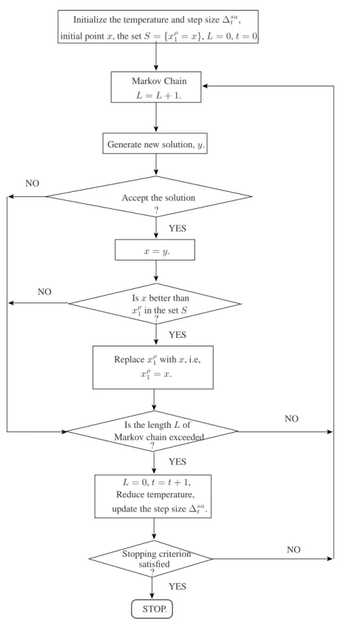
In this section, we present the full details of our main hybrid methods. The first hybrid method is similar to LSA except that it modifies the generation scheme of the LSA method. In particular, it uses the generation mechanism GM-I or GM-II and also updates the step size using equations (4.7)-(4.8). In addition, it keeps a record of the best point found using a singleton setSwhich is updated with a better point found in the Markov chain. This hybrid is referred to as the modified simulated annealing or MSA.

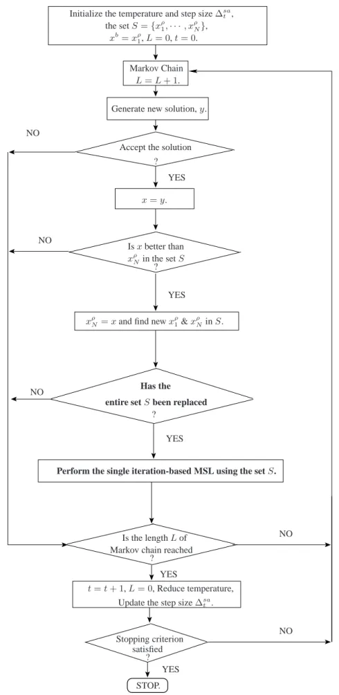
The second hybrid method extends MSA by incorporating the multi level single linkage (MSL) method [42] within the MSA method. It uses a setSconsisting ofNpoints, initially drawn uniformly in the search regionΩ. The setS is updated during the course of each Markov chain. This hybrid is referred to as the simulated annealing driven pattern search or SAPS.

4.2.1 Modified simulated annealing (MSA)

Like the LSA method, the MSA method initializes the pointxand the parameters of the cooling schedule before the beginning of the first Markov chain. The setSinitially contains the pointxρ₁ =x.

Structurally, like any other SA method, the MSA method has two loops. In the outer loop, the MSA method, not only decreases the temperature as in LSA, but also updates the step size parameter∆sa_t using equation (4.8). On the other hand, in the inner loop, MSA differs from LSA in that MSA uses the point generation mechanism GM-I or GM-II and updates the set S as soon as a better point is found in the Markov chain. Therefore the setScontains the best point visited by the MSA method.

(45)

4.2.1 Modified simulated annealing (MSA) 32 NO NO NO NO YES YES YES YES

Initialize the temperature and step size∆sa t ,

initial pointx, the setS={xρ1=x},L= 0,t= 0.

Markov Chain

L=L+ 1.

Generate new solution,y.

Accept the solution

? ? ? ? x=y. Isxbetter than xρ₁in the setS

Replacexρ₁withx, i.e,

xρ₁=x.

Is the lengthLof Markov chain exceeded

L= 0,t=t+ 1, Reduce temperature, update the step size∆sa

t .

Stopping criterion satisfied

STOP.

(46)

4.2.1 Modified simulated annealing (MSA) 33 The algorithm for MSA is presented below in Algorithm 4.1.

Algorithm 4.1: The MSA Algorithm.

1. Initialization : Generate an initial pointx. Setxρ₁ =x,xρ₁ _∈S. Set the temperature countert= 0. Compute the initial temperatureT0using equation (3.6). Calculate an initial step size parameter∆sa0

using equation (4.6).

2. The inner and outer loops:

while the stopping condition is not satisfied do begin

fori:= 1 toLdo begin

generateyfromxusing the mechanism in (4.1) or (4.3) ; iff(y)₋f(x)_≤0then accept;

else ifexp(₋(f(y)₋f(x) )/Tt)>random(0,1)then accept; if accept thenx=y;

update the setS, i.e., iff(x)< f(xρ₁)thenxρ₁ =x; end;

t:=t+ 1;

lowerTtusing equation (3.8) ; update∆sa

t using equation (4.8); end.

Remarks:

4.1. The stopping condition is given by equation (3.10).

4.2. The inner and outer loops of Algorithm 4.1 are similar to those of Algorithm 3.4, i.e., the LSA algo-rithm, but the significant changes are highlighted in bold.

Simulated annealing driven pattern search algorithms for global optimization