Andreas Groll & Gerhard Tutz
Regularization for Generalized Additive Mixed
Models by Likelihood-Based Boosting
Technical Report Number 110, 2011
Department of Statistics
University of Munich
Regularization for Generalized Additive Mixed Models
by Likelihood-Based Boosting
Andreas Groll
∗Gerhard Tutz
†June 29, 2011
Abstract
With the emergence of semi- and nonparametric regression the generalized linear mixed model has been expanded to account for additive predictors. In the present paper an approach to variable selection is proposed that works for generalized additive mixed models. In contrast to common procedures it can be used in high-dimensional settings where many covariates are available and the form of the influence is unknown. It is constructed as a componentwise boosting method and hence is able to perform variable selection. The complexity of the result-ing estimator is determined by information criteria. The method is investigated in simulation studies for binary and Poisson responses and is illustrated by using real data sets.
Keywords: Generalized additive mixed model, Boosting, Smoothing, Variable selection, Pe-nalized Quasi-Likelihood, Laplace approximation
∗Department of Statistics, University of Munich, Akademiestrasse 1, D-80799, Munich, Germany, email:
†Department of Statistics, University of Munich, Akademiestrasse 1, D-80799, Munich, Germany, email:
1
Introduction
General additive mixed models (GAMMs) are an extension of generalized additive models incorporating random effects. In the present article a boosting approach for the selection of additive predictors is proposed. Boosting originates in the machine learning community and turned out to be a successful and practical strategy to improve classification procedures by combining estimates with reweighted observations. The idea of boosting has become especially important in the last decade as the issue of estimating high-dimensional models has become more urgent. Since Freund and Schapire (1996) have presented their famous AdaBoost many extensions have been developed (e.g. gradient boosting by Friedman et al., 2000, generalized linear and additive regression based on theL2-loss by B¨uhlmann and Yu, 2003).
In the following the concept of likelihood-based boosting is extended to GAMMs which are sketched in Section 2. The fitting procedure is outlined in Section 3 and a simulation study is reported in Section 4. Finally, two applications are considered in Section 5.
2
Generalized Additive Mixed Models - GAMMs
Let yit denote observation t in cluster i, i = 1, . . . , n, t = 1, . . . , Ti, collected in yTi = (yi1, . . . , yiTi). Letx
T
it= (1, xit1, . . . , xitp) be the covariate vector associated with fixed effects
and zTit = (zit1, . . . , zitq) the covariate vector associated with random effects. It is assumed
that the observations yit are conditionally independent with means µit = E(yit|bi,xit,zit) and variancesvar(yit|bi) =φυ(µit), whereυ(.) is a known variance function and φis a scale parameter.
In addition to parametric effects the model that is considered includes an additive term that depends on covariatesuT
it= (uit1, . . . , uitm). The generalized semiparametric mixed model
that is assumed to hold is given by
g(µit) = xT itβββ+ m X j=1 α(j)(uitj) +zTitbi (1) = ηpar it +η add it +η rand it ,
where g is a monotonic differentiable link function, ηpar
it = xTitβββ is a linear parametric term with parameter vectorβββT = (β0, β1, . . . , βp), including the intercept,ηitadd=P
m
j=1α(j)(uitj) is
an additive term with unspecified influence functionsα(1), . . . , α(m) and finally ηrandit =zTitbi contains the cluster-specific random effects bi ∼ N(0,Q), where Q is a q×q dimensional
known or unknown covariance matrix. An alternative form that we also use in the following is µit=h(ηit), ηit=ηitpar+η add it +η rand it ,
whereh=g−1is the inverse link function. If the functionsα
(j)(·) are strictly linear, the model
reduces to the common generalized linear mixed model (GLMM). Versions of the additive model (1) have been considered by Zeger and Diggle (1994), Lin and Zhang (1999) and Zhang et al. (1998). While Lin and Zhang (1999) used natural cubic smoothing splines for the estimation of the unknown functionsα(j)(·), in the following regression splines are used. In recent years
regression splines have been widely used for the estimation of additive structures, see, for example, Marx and Eilers (1998), Wood (2004, 2006) and Wand (2000).
In regression spline methodology the unknown functionsα(j)(·) are approximated by basis
functions. A simple basis is known as the B-spline basis of degreed, yielding
α(j)(u) = k X i=1 α(ij)B (j) i (u;d),
whereB(ij)(u;d) denotes the i-th basis function for variablej. For an extensive discussion of smoothing by using splines, see for example Ruppert et al. (2003). More detailed information about the B-spline basis can be found for example in Eilers and Marx (1996).
In the following letαααT j = (α
(j)
1 , . . . , α
(j)
k ) denote the unknown parameter vector of the j -th smoo-th function and let BTj(u) = (B
(j)
1 (u;d), . . . , B
(j)
k (u;d)) represent the vector-valued evaluations of thekbasis functions. Then the parameterized model for (1) has the form
g(µit) =xTitβββ+BT1(uit1)ααα1+· · ·+BTm(uitm)αααm+zTitb.
By collecting observations within one cluster one obtains the design matrixXTi = (xi1, . . . ,xiTi)
for thei-th covariate, and analogously we setZTi = (zi1, . . . ,ziTi), so that the model has the
simpler form
g(µµµi) =Xiβββ+Bi1ααα1+· · ·+Bimαααm+Zibi,
where BTij = [Bj(ui1j), . . . ,Bj(uiTij)] denotes the transposed B-spline design matrix of the
i-th cluster and variable j and g is understood componentwise. Furthermore, let XT = [XT1, . . . ,XTn], letZ=diag(Z1, . . . ,Zn) be a block-diagonal matrix and letbT = (bT1, . . . ,bTn) be the vector collecting all random effects. Then one obtains the model in the matrix form
with BTj = [B T
1j, . . . ,B T
nj] representing the transposed B-spline design matrix of the j-th smooth function as in equation (17) in Appendix A. The model can be further reduced to
g(µµµ) =Xβββ+Bααα+Zb, (3)
whereαααT = (αααT
1, . . . , αααTm) andB= [B1, . . . ,Bm].
The Penalized Likelihood Approach
Focusing on generalized mixed models we assume that the conditional density of yit, given explanatory variables and the random effectbi, is of exponential family type
f(yit|xit,uit,bi) = exp
(y
itθit−κ(θit))
φ +c(yit, φ)
, (4)
where θit =θ(µit) denotes the natural parameter, κ(θit) is a specific function corresponding to the type of exponential family, c(.) the log normalization constant and φ the dispersion parameter (for example Fahrmeir and Tutz, 2001).
A popular method to maximize generalized mixed models is penalized quasi-likelihood (PQL), which has been suggested by Breslow and Clayton (1993), Lin and Breslow (1996) and Breslow and Lin (1995). In the following we briefly sketch the PQL approach for the semiparametric model. As common in mixed models, we assume that the covariance matrix Q(%%%) of the random effectsbi may depend on an unknown parameter vector%%%which specifies the correlation. We specify the joint likelihood-function by the parameters of the covariance structure%%%together with the dispersion parameter φ, which are collected inνννT = (φ, %%%T) and define the parameter vectorδδδT = (βββT, αααT,bT). The corresponding log-likelihood is
l(δδδ, ννν) = n X i=1 log Z f(yi|δδδ, ννν)p(bi, ννν)dbi . (5)
To avoid too severe restrictions on the form of the functionsα(j)(·), we use many basis functions,
say about 20 for each functionα(j)(.), and add a penalty term to the log-likelihood. Then one
obtains the penalized log-likelihood
lpen(δδδ, ννν) = n X i=1 log Z f(yi|δδδ, ννν)p(bi, ννν)dbi −12 m X j=1 λjαααTjKjαααj, (6)
where Kj penalizes the parameters αααj and λj are smoothing parameters which control the influence of thej-th penalty term. When using P-splines one penalizes the difference between adjacent categories in the formλjαααTjKjαααj=λjαααjT(∆∆∆d)T∆∆∆dαααj, where ∆∆∆ddenotes the difference
operator matrix of degree d, for details see, for example, Eilers and Marx (1996). The log-likelihood (6) has also been considered by Lin and Zhang (1999) but with Kj referring to smoothing splines. For smoothing splines the dimension of αααj increases with sample size whereas for the low rank smoother used here the dimension does not depend onn.
By approximating the likelihood in (6) along the lines of Breslow and Clayton (1993) one obtains the double penalized log-likelihood:
lpen (δδδ, ννν) = n X i=1 log(f(yi|δδδ, ννν))−12 n X i=1 bTiQ(%%%)−1bi− 1 2 m X j=1 λjαααTjKjαααj, (7)
where the first penalty term Pni=1bTi Q(%%%)−1bi is due to the approximation based on the Laplace method and the second penalty termPmj=1λjαααTjKjαααj determines the smoothness of the functionsα(j)(.), depending on the chosen smoothing parameterλj.
PQL usually works within the profile likelihood concept. It is distinguished between the estimation ofδδδ, given the plug-in estimate ˆννν, resulting in the profile-likelihoodlpen(δδδ,νννˆ), and
the estimation ofννν. The PQL method for generalized additive mixed models is implemented in thegamm function of the R-packagemgcv (Wood, 2006). Further aspects were discussed by Wolfinger and O’Connell (1993), Littell et al. (1996) and Vonesh (1996).
Note that the double penalized log-likelihood from equation (7) can also be derived by an EM-type algorithm, using posterior modes and curvatures instead of posterior means and covariances (see, for example, Fahrmeir and Tutz, 2001).
3
Boosted GAMMs -
bGAMM
Boosting originates in the machine learning community and turned out to be a successful and practical strategy to improve classification procedures by combining estimates with reweighted observations. The idea of boosting has become more and more important in the last decade as the issue of estimating high-dimensional models has become more urgent. Since Freund and Schapire (1996) have presented their famous AdaBoost many other variants in the framework of functional gradient descent optimization have been developed (for example Friedman et al., 2000 or Friedman, 2001). B¨uhlmann and Yu (2003) further extended boosting to generalized linear and additive regression problems based on theL2-loss.
Boosting is especially successful as a method to select relevant predictors in linear and generalized linear models. For extensions to GLMMs, see Tutz and Groll (2011). It works by iterative fitting of residuals using “weak learners”. The boosting algorithm that is presented in the following extends the method to additive mixed models.
3.1
The Boosting Algorithm
The following algorithm uses componentwise boosting, that is, only one component of the additive predictor, in our case one weight vectorαααj, is fitted at a time. That means that a model containing the linear term and only one smooth component is fitted in one iteration step. We use a reparametrization technique explained in more detail in Appendix A. The B-spline design matricesBjfrom equation (2), corresponding to the difference penalty matricesKj and spline coefficientsαααj, can be transformed to new design matrices ΦΦΦj with spline coefficients ˜
α
ααj, which consist of an unpenalized and a penalized part and correspond to diagonal penalty matrices ˜K := ˜Kj = diag(0, . . . ,0,1, . . . ,1), which are equal for all j = 1, . . . , m. We drop the first column of each matrix ΦΦΦj, because we are in the semiparametric model context (see Appendix B).
The predictor containing all covariates associated with fixed effects and only the covariate vector of ther-th smooth effect yields for clusteri
ηηηi·r=Xiβββ+ ΦΦΦirααα˜r+Zibi,
where ΦΦΦiris a sub-matrix of ΦΦΦr, consisting of only theTirows from ΦΦΦrcorresponding to cluster i. Altogether the predictor, considering only ther-th smooth effect, has the form
ηηη··r=Xβββ+ ΦΦΦr˜αααr+Zb.
Moreover, we define ΦΦΦ := [ΦΦΦ1, . . . ,ΦΦΦm] and introduce the new parameter vector γγγT :=
(βββT,ααα˜T,bT). The following boosting algorithm uses the EM-type algorithm given in Fahrmeir and Tutz (2001). We further want to introduce the vectorγγγT
r := (βββ T
,ααα˜Tr,bT), containing only the spline coefficients of ther-th smooth component.
Algorithm bGAMM
1. Initialization
Compute starting values ˆβββ(0),αααˆ˜(0),bˆ(0),Qˆ(0) and set ˆηηη(0)=Xβββˆ(0)+ ΦΦΦˆααα˜(0)+Zbˆ(0).
2. Iteration
Forl= 1,2, . . .
(a) Refitting of residuals
Forr∈ {1, . . . , m} the model
g(µµµ) = ˆηηη(l−1)+Xβββ+ ΦΦΦr˜αααr+Zb
is fitted, where ˆηηη(l−1) = Xβββˆ(l−1)+ ΦΦΦˆααα˜(l−1)+Zbˆ(l−1) is considered a known
off-set. Estimation refers toγγγT r = (βββ
T
,ααα˜Tr,bT). In order to obtain an addi-tive correction of the already fitted terms, we use one-step Fisher scoring with starting valueγγγr =0. Therefore Fisher scoring for ther-th component takes the simple form
ˆ γγγ(rl)= (F pen r (ˆγγγ (l−1) ))−1sr(ˆγγγ(l−1)) (8)
with penalized pseudo Fisher matrixFpen
r (γγγ) and using the unpenalized version of the penalized score functionspen
r (γγγ) =∂lpen(γγγ)/∂γγγr(see Section 3.2.1). The variance-covariance components are replaced by their current estimates ˆQ(l−1). (ii.) Selection step
Select fromr∈ {1, . . . , m}the componentjthat leads to the smallestAICr(l)or BICr(l) as given in Section 3.2.3 and select the corresponding vector (ˆγγγ(jl))T =
(ˆβββ∗)T,(ˆααα˜∗ j)T,(ˆb ∗ )T. (iii.) Update Set ˆ βββ(l)= ˆβββ(l−1)+ ˆβββ∗, bˆ(l)= ˆb(l−1)+ ˆb∗
and forr= 1, . . . , m set
ˆ ˜ α α α(rl)= ˆ ˜ α αα(rl−1) if r6=j ˆ ˜ α αα(rl−1)+ ˆααα˜∗r if r=j, (ˆγγγ(l))T = (ˆβββ(l))T,(ˆααα˜1(l))T, . . . ,(ˆααα˜(ml))T,(ˆb (l) )T . WithA:= [X,ΦΦΦ,Z] update ˆ ηηη(l)=Aˆγγγ(l)
(b) Computation of variance-covariance components
Estimates of ˆQ(l)are obtained as approximate REML-type estimates or alternative methods (see Section 3.2.2)
Note that the EM-type algorithm may be viewed as an approximate EM algorithm, where the posterior ofbi is approximated by a normal distribution. In the case of linear random effects
models, the EM-type algorithm corresponds to an exact EM algorithm since the posterior ofbi is normal, and so posterior mode and mean coincide, as do posterior covariance and curvature.
3.2
Computational details of
bGAMM
In the following we give a more detailed description of the single steps of thebGAMMalgorithm. First the derivation of the score function and the Fisher matrix are described. Then we present two estimation techniques for the variance-covariance components, give the details of the computation of the starting values and explain the selection procedure.
3.2.1 Score Function and Fisher Matrix
In this section we specify more precisely the single components which are derived in step 2 (a) of thebGAMM algorithm. Forr∈ {1, . . . , p} the penalized score functionsspen
r (γγγ) are obtained by differentiating the penalized log-likelihood from equation (7) with respect toγγγr, that is spen
r (γγγ) =∂lpen(γγγ)/∂γγγr. To keep the notation simple, we omit the argumentγγγ in the following
and writespen(l−1)
r = (spen(l−1) β β βr )T,(s pen(l−1) ˜ αααrr ) T,(spen(l−1) 1r )T, . . . ,(s pen(l−1) nr )T T =spen r (ˆγγγ (l−1) ) for ther-th evaluated penalized score function at (l−1)-th iteration. For givenQ, it has single components spen(l−1) β ββr = n X i=1 XTi DiΣΣΣ−i1(yi−µµµˆi), spen(l−1) ˜ α ααrr = n X i=1 Φ Φ ΦTirDiΣΣΣ−i1(yi−µµµˆi)−λK˜αααˆ˜(rl−1), spenir (l−1) = Z T iDiΣΣΣ−i1(yi−µµµˆi)−Q− 1ˆ b(il−1), i= 1, . . . , n,
withDi =∂h(ˆηηηi)/∂ηηη,ΣΣΣi =cov(yi), and ˆµµµi =h(ˆηηηi) evaluated at previous fit ˆηηηi =Aiˆγγγ
(l−1)
, whereas Ai := [Xi,ΦΦΦi,Zi]. One should keep in mind that actually, Di,ΣΣΣi, µµµi and ηηηi are depending on ˆγγγ(l−1) and thus on the current iteration, which is suppressed here to keep the notation simple. The vectorsβpenββr (l−1)has dimension p+ 1, the vectors
pen(l−1) ˜
α α
αrr has dimension
kcorresponding to the number of basis functions, while the vectorsspenir (l−1)are of dimension s. Note thatspen(l−1)
r could be seen as penalized score function because of the termsλK˜αααˆ˜(rl−1) andQ−1bˆ(il−1).
Let ˜βββTr := (βββ T
,ααα˜Tr). Then the penalized pseudo Fisher matrixF
pen(l−1)
which is partitioned into Fpen(l−1) r = Fββ˜β rβββ˜rr Fββ˜βr1r Fβββ˜r2r . . . Fβββ˜rnr F1˜βββ rr F11r 0 F2˜βββ rr F22r .. . . .. Fnβββ˜rr 0 Fnnr , with Fβββ˜ rβββ˜rr= Fββββββr Fβββααα˜rr Fααα˜rβββr Fααα˜rααα˜rr ,
has single components
Fββββββr = −E ∂2lpen ∂βββ∂βββT = n X i=1 XTi DiΣΣΣ−i1DiXi Fβββααα˜rr = F T ˜ αααrβββr=−E ∂2lpen ∂βββ∂ααα˜Tr = n X i=1
XTiDiΣΣΣ−i 1DiΦΦΦir,
Fααα˜rααα˜rr = −E ∂2lpen ∂ααα˜r∂ααα˜Tr = n X i=1 Φ
ΦΦTirDiΣΣΣi−1DiΦΦΦir−λK˜, Fβββ˜ rir = F T iβββ˜rr=−E ∂2lpen ∂βββ˜r∂bTi !
= [Xi,ΦΦΦir]TDiΣΣΣ−i1DiZi,
Fiir = −E ∂2lpen ∂bi∂bTi =ZTi DiΣΣΣ−i1DiZi+Q− 1.
whereasDi=∂h(ˆηηηi)/∂ηηηand ΣΣΣi =cov(yi) again are evaluated at the previous fit ˆηηηi=Aiˆγγγ
(l−1)
. 3.2.2 Variance-Covariance Components
In this section we present two different ways how to perform the update of the variance-covariance matrixQfrom step 2. (b) of the ourbGAMMalgorithm.
Breslow and Clayton (1993) recommend to estimate the variance by maximizing the profile likelihood that is associated with the normal theory model. By replacingβββ andαααwith ˆβββ and ˆ α ααwe maximize l(Qb) = − 1 2log(|V(ˆγγγ)|)− 1 2log(|[X,ΦΦΦ] TV−1(ˆγγγ)[X,ΦΦΦ] |) −12(˜ηηη(ˆγγγ)−Xββˆβ−ΦΦΦˆααα)TV−1(ˆγγγ)(˜ηηη(ˆγγγ)−Xβββˆ−ΦΦΦˆααα) (9) with respect toQb, using the pseudo-observations ˜ηηη(γγγ) =Aγγγ+D−1(γγγ)(y−µµµ(γγγ)) and with matrices V(γγγ) = W−1(γγγ) +ZQbZT, W(γγγ) = D(γγγ)ΣΣΣ−1(γγγ)D(γγγ)T and with block-diagonal matricesQb=diag(Q, . . . ,Q), D=diag(D1, . . . ,Dn) and ΣΣΣ =diag(ΣΣΣ1, . . .ΣΣΣn). Having
cal-culated ˆγγγ(l)in thel-th boosting iteration, we obtain the estimator ˆQ(bl), which is an approximate REML-type estimate forQb.
An alternative estimate, that can be derived as an approximate EM algorithm, uses the posterior mode estimates and posterior curvatures. One derives (Fpen(l))−1, the inverse of the
penalized pseudo Fisher matrix of the full model corresponding to thel-th iteration using the posterior mode estimates ˆγγγ(l)to obtain the posterior curvatures ˆV(iil). Now compute ˆQ
(l) by ˆ Q(l)= 1 n n X i=1 ( ˆV(iil)+ ˆb (l) i (ˆb (l) i )T). (10)
In general, theVii are derived via the formula
Vii =F−ii1+F−ii1Fiββ˜β(Fβββ˜ββ˜β− n X i=1 Fβ˜ββiF− 1 ii Fiβββ˜)− 1F ˜ β ββiF− 1 ii ,
whereas ˜βββT := (β, αββ ααJ1, . . . , αααJs) and J = {j : sign(αααj) 6= 0, j = 1, . . . , m} is the index set
of “active” covariates, corresponding to the s:= #J ≤mnon-zero spline coefficient vectors. Fβββ˜ββ˜β,Fiβββ˜,Fii are the elements of the penalized pseudo Fisher matrixFpen of the full model
corresponding to thel-th iteration, for details see for example Tutz and Hennevogl (1996) or Fahrmeir and Tutz (2001).
3.2.3 Starting Values, Hat Matrix and Selection in bGAMM
We compute the starting values ˆβββ(0),αααˆ˜(0),bˆ(0),Qˆ(0) from step 1 of the bGAMM algorithm by
setting ˆααα˜(0)= 000 and then fitting a GLMM given by
g(µit) =xT
itβββ+zTitbi, i= 1, . . . , n; t= 1, . . . , Ti. (11)
This model can be fitted e.g. by using the R-function glmmPQL(Wood, 2006) from theMASS
library (Venables and Ripley, 2002).
To find the appropriate complexity of our model we use the effective degrees of free-dom, which corresponds to the trace of the hat matrix (Hastie and Tibshirani, 1990). In the following we derive the hat matrix corresponding to the l-th boosting step for the r -th smoo-th component (compare Tutz and Groll, 2011). Let A..r := [X,ΦΦΦr,Z] and ΛΛΛ = diag(0, . . . ,0,K˜,Q−1, . . . ,Q−1) be a block diagonal penalty matrix with a diagonal consisting ofp+ 1 zeros corresponding to the fixed effects at the beginning, followed by ˜Kcorresponding to ther-th smooth effect and finallyntimes the matrixQ−1. Then the Fisher matrixFpen(l−1)
r and the score vectorspen(l−1)
r are given in closed form as
Fpen(l−1)
and
spen(l−1)
r =AT··rWlD−l 1(y−µµˆµ
(l−1))
−ΛΛΛˆγγγ(rl−1)
whereWl,Dl,ΣΣΣland ˆµµµ(l−1)are evaluated at the previous fit ˆηηη(l−1)=Aˆγγγ(l−1). Forr= 1, . . . , p the refit in thel-th iteration step by Fisher scoring (8) is given by
ˆ γγγ(rl) = (F pen(l−1) r )−1s(rl−1) = AT..rWlA··r+ ΛΛΛ −1 AT..rWlD−l1(y−µµµˆ (l−1)).
We define the predictor corresponding to ther-th refit in thel-th iteration step as
ˆ ηηη(..rl) := ηηηˆ (l−1) +A..rˆγγγ(rl), ˆ ηηη(..rl)−ηηηˆ(l−1) = A..rγγγˆ(rl) = A..rAT..rWlA··r+ ΛΛΛ −1 AT..rWlD− 1 l (y−µµµˆ (l−1) ).
Taylor approximation of first orderh(ˆηηη)≈h(ηηη) +∂h∂ηηη(Tηηη)(ˆηηη−ηηη) yields
ˆ µ µµ(··lr) ≈ µµµˆ(l−1)+Dl(ˆηηη(..rl)−ηηηˆ(l−1)), ˆ ηηη(··lr)−ηηηˆ (l−1) ≈ D−l 1(ˆµµµ (l) ..r−µµµˆ (l−1) ), and therefore Dl−1(ˆµµµ··(lr)−µµµˆ(l−1))≈A..r AT..rWlA..r+ ΛΛΛ −1 AT..rWlD−l 1(y−µµµˆ (l−1)).
Multiplication withW1l/2 and usingW1/2D−1= ΣΣΣ−1/2yields
ΣΣΣ−l1/2(ˆµµµ(..rl)−µµµˆ (l−1) )≈H˜(rl)ΣΣΣ− 1/2 l (y−µµµˆ (l−1) ), where ˜H(rl) := W 1/2 l A..r AT..rWlA..r+ ΛΛΛ −1 AT..rW 1/2
l denotes the usual generalized ridge regression hat-matrix. DefiningM(rl):= ΣΣΣ1l/2H˜(rl)ΣΣΣ−l 1/2yields the approximation
ˆ µ µµ(..rl) ≈ µµµˆ (l−1) +M(rl)(y−µµµˆ (l−1) ) = µµµˆ(l−1)+M(rl)[(y−µµµˆ (l−2) )−(ˆµµµ(l−1)−µµµˆ(l−2))] ≈ µµµˆ(l−1)+M(rl)[(y−µµµˆ (l−2) )−Mj(ll−−11)(y−µµµˆ (l−2) )],
The hat matrix corresponding to the fixed effects model from equation (11) is
M(0)=A0(AT0W1A0+K0)−1AT0W1,
with A0 := [X,Z] and block diagonal penalty matrix K0 := diag(0, . . . ,0,Q−1, . . . ,Q−1)
whereas the firstp+1 zeros correspond to the fixed effects. As the approximation ˆµµµ(0) ≈M(0)y holds, one obtains
ˆ µ µ µ(1)..r ≈ µµµˆ(0)+M(1)r (y−µµµˆ(0)) ≈ M(0)y+M(1)r (I−M (0) )y.
In the following, to indicate that the hat matrices of the former steps have been fixed, let
jk ∈ {1, . . . , p} denote the index of the component selected in boosting step k. Then we can
abbreviateMjk :=M
(k)
jk for the matrix corresponding to the component that has been selected
in thek-th iteration. Further, in a recursive manner, we get
ˆ µµµ(..rl)≈H(rl)y, where H(rl) = I−(I−M (l) r )(I−Mjl−1)(I−Mjl−2)·. . .·(I−M (0) ) = M(rl) l−1 Y i=0 (I−Mji) + l−1 X k=0 Mjk kY−1 i=0 (I−Mji) = l X k=0 Mjk kY−1 i=0 (I−Mji),
is the hat matrix corresponding to the l-th boosting step considering the r-th component, whereasMjl :=M
(l)
r is not fixed yet.
For a given hat matrixH, we can determine the complexity of our model by the following information criteria:
AIC = −2l(ˆµµµ) + 2 trace (H), (12) BIC = −2l(ˆµµµ) + 2 trace (H)log(n), (13)
where l(µµµ) = n X i=1 li(ˆµµµi) = n X i=1 logf(yi|µµˆµi) (14) denotes the non-penalized version of the log-likelihood from equation (7) andli(ˆµµµi) the
log-likelihood contributions of (yi,Xi,ΦΦΦi,Zi). Note that the log-likelihood can be written withµµµ instead ofδδδ in the argument, considering the definition of the natural parameterθ=θ(µµµ) in (4) and usingµµµ=h(ηηη) andηηη=Aγγγ.
For exponential family distributions logf(yi|µµµˆi) has a well-known form. For example in the case of binary responses, one obtains
logf(yi|µµµˆi) = Ti
X
t=1
yitlog ˆµit+ (1−yit) log (1−µˆit),
whereas in the case of Poisson responses, one has
logf(yi|µµˆµi) = Ti
X
t=1
yitlog ˆµit−µˆit.
Based on (14), the information criteria (12) and (13) used in thel-th boosting step, considering ther-th component, have the formAICr(l)=−2l(ˆµµµ(..rl)) + 2 trace (H(rl)),BIC
(l)
r =−2l(ˆµµµ(..rl)) + 2 trace (H(rl))log(n) withl(ˆµµµ
(l) ..r) = Pn i=1logf(yi|µµˆµ (l) i.r). 3.2.4 Stopping Criterion
In the l-th step one selects from r ∈ {1, . . . , p} the component jl that minimizes AICr(l) or BICr(l) and obtains AIC(l) := AICj(ll). We choose a number lmax of maximal boosting steps, e.g. lmax = 1000, and stop the algorithm at iteration lmax. Then we select from L:={1,2, . . . , lmax} the componentlopt, whereAIC(l) orBIC(l)is smallest, that is
lopt = arg min l∈L
AIC(l), lopt = arg min
l∈L
BIC(l).
Finally, we obtain the parameter estimates ˆγγγ(lopt),Qˆ(lopt)and the corresponding fit ˆµµµ(lopt).
4
Simulation study
In the following we present two simulation studies to investigate the performance of thebGAMM
algorithm, one with Bernoulli data and one with Poisson data. We also compare the algorithm to alternative approaches. The optimal smoothing parameterλchosen as the valueλoptwhich leads to the smallestAICorBICfrom (12) and (13), which are computed on a fine grid. Also general cross validation could be used, with the negative effect of expanding computational time.
4.1
Bernoulli Data with Logit-Link
The underlying model is the random intercept additive Bernoulli model
ηit =
p
X
j=1
fj(uitj) +bi, i= 1, . . . ,40, t= 1, . . . ,10
E[yit] = exp(ηit)
1 + exp(ηit) :=πit yit∼B(1, πit) with smooth effects given by
f1(u) = 6 sin(u) with u∈[−π, π], f2(u) = 6 cos(u) with u∈[−π,2π], f3(u) =u2 with u∈[−π, π], f4(u) = 0.4u3 with u∈[−π, π], f5(u) =−u2 with u∈[−π, π], fj(u) = 0 with u∈[−π, π], for j = 6, . . . ,50.
We choose the different settings p = 5,10,15,20,50. For j = 1, . . . ,50 the vectors uT it =
(uit1, . . . , uit50) have been drawn independently with components following a uniform
distri-bution within the specified interval. The number of observations is fixed as n = 40, Ti :=
T = 10,∀i= 1, . . . , n. The random effects are specified by bi ∼N(0, σb2) with three different
scenariosσb ∈ {0.4,0.8,1.6}.
The performance of estimators is evaluated separately for the structural components and the variance. We compare the results of ourbGAMMalgorithm with the results that one achieves by using theR functiongamm recommended in Wood (2006), which is providing a penalized quasi-likelihood approach for the generalized additive mixed model. It is supplied with the
mgcvlibrary.
By averaging across 100 data sets we consider mean squared errors for the smooth compo-nents andσb given by
msef := N X t=1 p X j=1 (fj(vtj)−fˆj(vtj))2, mseσb :=||σb−ˆσb|| 2,
where vtj, t= 1, . . . , N denote fine and evenly spaced grids on the different predictor spaces forj = 1, . . . , p.
Additional information on the stability of the algorithms was collected innotconv (n.c.), which indicates the sum over the datasets, where numerical problems occurred during estima-tion. Moreover, falseneg (f.n.) reflects the mean over all 100 simulations of the number of
functionsfj, j= 1,2,3,4,5, that were not selected whilefalsepos (f.p.) reflects the mean over the number of functionsfj, j= 6, . . . , p, that were wrongly selected. As thegamm function is not able to perform variable selection it always estimates all functionsfj, j= 1, . . . , p.
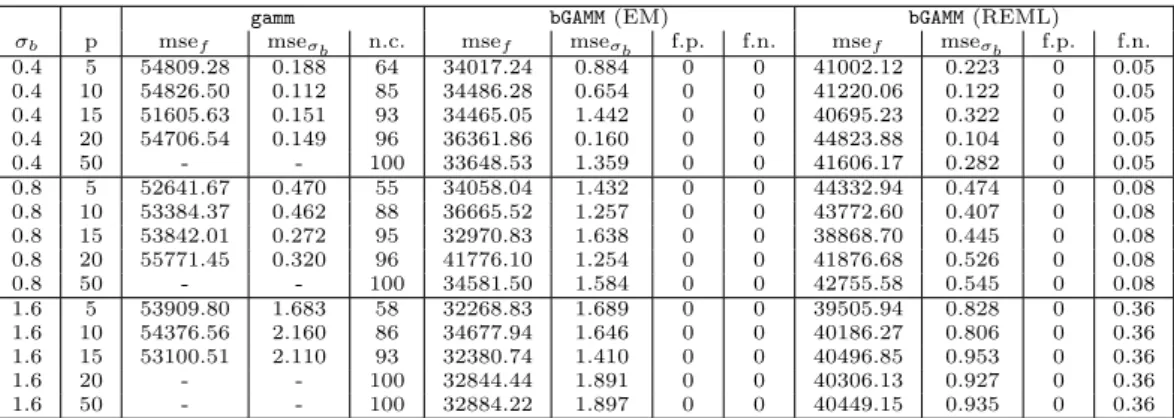
The results of all quantities for different scenarios of σb and for varying number of noise variables can be found in Table 1. It should be noted that, in order to obtain a better compa-rability, the quantities msef and mseσb are only averaged across those cases, where thegamm
function yields reasonable results, while the quantitiesnotconv, falseneg and falsepos are av-eraged across all 100 simulations. Also the following boxplots include only those cases, where no numerical problems occurred for thegamm function, see Figures 1 and 2.. For completeness we give the results of thebGAMM algorithm averaged over all 100 simulations in the Table 2.
gamm bGAMM(EM) bGAMM(REML)
σb p msef mseσb n.c. msef mseσb f.p. f.n. msef mseσb f.p. f.n.
0.4 5 54809.28 0.188 64 34017.24 0.884 0 0 41002.12 0.223 0 0.05 0.4 10 54826.50 0.112 85 34486.28 0.654 0 0 41220.06 0.122 0 0.05 0.4 15 51605.63 0.151 93 34465.05 1.442 0 0 40695.23 0.322 0 0.05 0.4 20 54706.54 0.149 96 36361.86 0.160 0 0 44823.88 0.104 0 0.05 0.4 50 - - 100 33648.53 1.359 0 0 41606.17 0.282 0 0.05 0.8 5 52641.67 0.470 55 34058.04 1.432 0 0 44332.94 0.474 0 0.08 0.8 10 53384.37 0.462 88 36665.52 1.257 0 0 43772.60 0.407 0 0.08 0.8 15 53842.01 0.272 95 32970.83 1.638 0 0 38868.70 0.445 0 0.08 0.8 20 55771.45 0.320 96 41776.10 1.254 0 0 41876.68 0.526 0 0.08 0.8 50 - - 100 34581.50 1.584 0 0 42755.58 0.545 0 0.08 1.6 5 53909.80 1.683 58 32268.83 1.689 0 0 39505.94 0.828 0 0.36 1.6 10 54376.56 2.160 86 34677.94 1.646 0 0 40186.27 0.806 0 0.36 1.6 15 53100.51 2.110 93 32380.74 1.410 0 0 40496.85 0.953 0 0.36 1.6 20 - - 100 32844.44 1.891 0 0 40306.13 0.927 0 0.36 1.6 50 - - 100 32884.22 1.897 0 0 40449.15 0.935 0 0.36
Table 1: Generalized additive mixed model withgammand boosting (bGAMM) on Bernoulli data
bGAMM(EM) bGAMM(REML)
σb p msef mseσb msef mseσb
0.4 5 33563.44 1.382 41671.53 0.280 0.4 10 33563.44 1.382 41671.53 0.280 0.4 15 33563.44 1.382 41671.53 0.280 0.4 20 33530.58 1.395 41624.79 0.282 0.4 50 33648.53 1.359 41606.17 0.282 0.8 5 34581.50 1.584 42755.58 0.545 0.8 10 34581.50 1.584 42755.58 0.545 0.8 15 34581.50 1.584 42755.58 0.545 0.8 20 34581.50 1.584 42755.58 0.545 0.8 50 34581.50 1.584 42755.58 0.545 1.6 5 32844.44 1.891 40306.13 0.927 1.6 10 32844.44 1.891 40306.13 0.927 1.6 15 32844.44 1.891 40306.13 0.927 1.6 20 32844.44 1.891 40306.13 0.927 1.6 50 32884.22 1.897 40449.15 0.935
Table 2: Generalized additive mixed model with boosting (bGAMM) on bernoulli data averaged over all 100 simulations
It is seen that thegammfunction is very unstable when the number of predictors grows and for all numbers of predictors estimates are hard to find. The boosting algorithms are much more stable and msefis even better if evaluated for all simulations instead of the subset favored bygamm. So for binary data boosting procedures dominategammin terms of msef. In terms of
mseσb gammdominates but the REML version of boosting comes close.
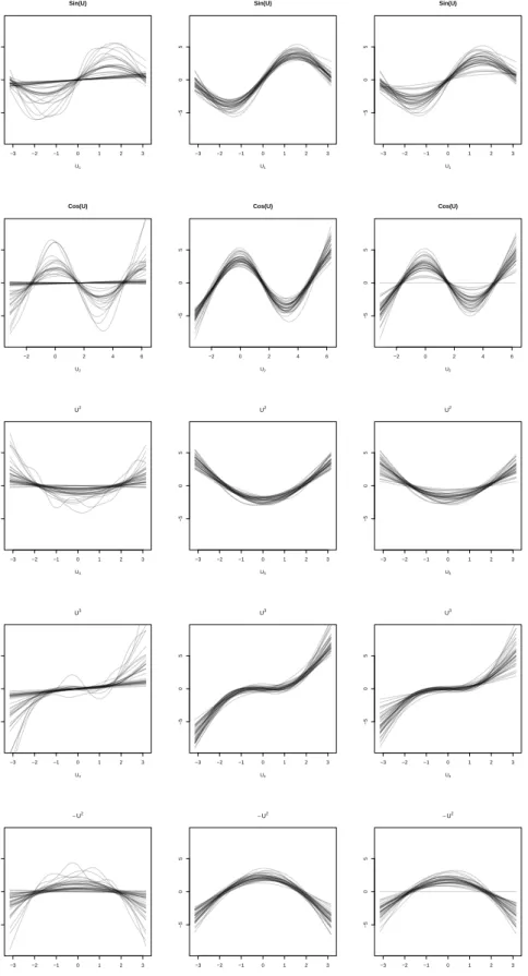
Exemplarily for the case p = 5 and σb = 0.4 the estimates of the smooth functions are presented in Figure 3 for those 36 simulations, where the gamm function estimated without numerical problems. It becomes obvious that the two boosting approaches can reproduce the true feature of the influence functions much more precisely, with the EM version leading to slightly better results.
● ● ●● ● ● p=5 p=10 p=15 p=20 p=50 30000 40000 50000 60000 70000 80000 gamm ● ● ● ● ● ● ● ● ● ● p=5 p=10 p=15 p=20 p=50 30000 40000 50000 60000 70000 80000 bGAMM (EM) ● ● ● ● ● ● ● ● ● ● p=5 p=10 p=15 p=20 p=50 30000 40000 50000 60000 70000 80000 bGAMM (REML)
Figure 1: Boxplots of msef forgamm∗ (left), bGAMM EM(middle) and bGAMM REML (right) for p=
5,10,15,20,50 (∗only those cases, wheregammdid converge)
● ● ● ● ● ●●● ● ● ● ● ● ● ● p=5 p=10 p=15 p=20 p=50 0 1 2 3 4 5 6 gamm ● ● ● ● ● p=5 p=10 p=15 p=20 p=50 0 1 2 3 4 5 6 bGAMM (EM) ● ●● ● ● ● ● ● ● ● ● ● ● ● ● ● ●● ● ●● ● ● ● ● ● ● ● ● ● ● ● ● ● ●● ● ●● ● ● ● ● ● ● ● ● ● ● ● ● ● ●● ● ●● ● ● ● ● ● ● ● ● ● ● ● ● ● ●● ● ●● ● ● ● ● ● ● ● ● ● ● ● ● ● ●● p=5 p=10 p=15 p=20 p=50 0 1 2 3 4 5 6 bGAMM (REML)
Figure 2: Boxplots of mseσ for thegammmodel (left), thebGAMMEM model (middle) and thebGAMM
−3 −2 −1 0 1 2 3 −5 0 5 Sin(U) U1 −3 −2 −1 0 1 2 3 −5 0 5 Sin(U) U1 −3 −2 −1 0 1 2 3 −5 0 5 Sin(U) U1 −2 0 2 4 6 −5 0 5 Cos(U) U2 −2 0 2 4 6 −5 0 5 Cos(U) U2 −2 0 2 4 6 −5 0 5 Cos(U) U2 −3 −2 −1 0 1 2 3 −5 0 5 U2 U3 −3 −2 −1 0 1 2 3 −5 0 5 U2 U3 −3 −2 −1 0 1 2 3 −5 0 5 U2 U3 −3 −2 −1 0 1 2 3 −5 0 5 U3 U4 −3 −2 −1 0 1 2 3 −5 0 5 U3 U4 −3 −2 −1 0 1 2 3 −5 0 5 U3 U4 −3 −2 −1 0 1 2 3 −5 0 5 −U2 U5 −3 −2 −1 0 1 2 3 −5 0 5 −U2 U5 −3 −2 −1 0 1 2 3 −5 0 5 −U2 U5
Figure 3: Smooth functions computed with thegammmodel (left), thebGAMMEM model (middle) and
4.2
Poisson Data with Log-Link
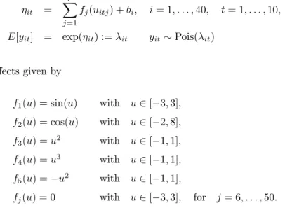
The underlying model is the random intercept additive Poisson model
ηit =
p
X
j=1
fj(uitj) +bi, i= 1, . . . ,40, t= 1, . . . ,10, E[yit] = exp(ηit) :=λit yit∼Pois(λit)
with smooth effects given by
f1(u) = sin(u) with u∈[−3,3], f2(u) = cos(u) with u∈[−2,8], f3(u) =u2 with u∈[−1,1], f4(u) =u3 with u∈[−1,1], f5(u) =−u2 with u∈[−1,1], fj(u) = 0 with u∈[−3,3], for j= 6, . . . ,50.
Again we choose the different settings p = 5,10,15,20,50. For j = 1, . . . ,50 the vectors uT
it = (uit1, . . . , uit50) have been drawn independently with components following a uniform
distribution within the specified interval. The number of observations is fixed asn= 40, Ti:=
T = 10,∀i = 1, . . . , n. The random effects are specified by bi ∼ N(0, σ2b) with same three
scenarios as in the Poisson case.
We also use the same goodness-of-fit criteria as for the Bernoulli case and compare the results of ourbGAMM algorithm with the results achieved by using thegamm function (Wood, 2006), see Table 3.
gamm bGAMM(EM) bGAMM(REML)
σb p msef mseσb n.c. msef mseσb f.p. f.n. msef mseσb f.p. f.n.
0.4 5 21.220 0.004 0 28.617 0.050 0 0 28.598 0.005 0 0 0.4 10 26.059 0.004 39 28.158 0.033 0.01 0 28.158 0.005 0.02 0 0.4 15 27.819 0.003 89 23.927 0.100 0.04 0 23.968 0.007 0.04 0 0.4 20 33.050 0.001 95 28.259 0.027 0.04 0 28.278 0.004 0.04 0 0.4 50 79.245 0.006 89 32.522 0.029 0.09 0 30.899 0.005 0.08 0 0.8 5 19.398 0.010 0 24.293 0.122 0 0 24.310 0.009 0 0 0.8 10 21.859 0.011 48 23.827 0.097 0.01 0 23.836 0.007 0.01 0 0.8 15 36.088 0.001 96 26.524 0.151 0.01 0 26.560 0.002 0.01 0 0.8 20 36.311 0.007 95 25.704 0.015 0.02 0 25.652 0.007 0.02 0 0.8 50 75.365 0.015 95 25.258 0.177 0.06 0 23.526 0.009 0.06 0 1.6 5 11.823 0.038 2 15.301 1.224 0 0 15.283 0.042 0 0 1.6 10 14.869 0.036 57 16.229 1.287 0.14 0 16.283 0.040 0.14 0 1.6 15 14.098 0.070 99 4.478 7.212 0.22 0 4.481 0.127 0.23 0 1.6 20 - - 100 16.762 1.139 0.28 0 16.818 0.042 0.28 0 1.6 50 2043.006 2.543 99 34.449 0.963 0.46 0 27.338 0.044 0.47 0
Table 3: Generalized additive mixed model withgammand boosting (bGAMM) on Poisson data
For completeness we give the results of thebGAMM algorithm averaged over all 100 simula-tions in the Table 4. For Poisson data it is seen again that thegamm function is very unstable
when the number of predictors grows. Already for ten predictors estimates are hard to find. The boosting algorithms are much more stable and msef is again better if evaluated for all simulations instead of the subset favored bygamm.
bGAMM(EM) bGAMM(REML)
σb p msef mseσb msef mseσb
0.4 5 28.617 0.050 28.598 0.005 0.4 10 28.597 0.050 28.732 0.005 0.4 15 28.888 0.050 28.927 0.005 0.4 20 28.863 0.050 28.869 0.005 0.4 50 29.391 0.050 28.848 0.005 0.8 5 24.293 0.122 24.310 0.009 0.8 10 24.346 0.121 24.364 0.009 0.8 15 24.360 0.121 24.377 0.009 0.8 20 24.465 0.118 24.456 0.009 0.8 50 24.899 0.113 24.464 0.009 1.6 5 15.301 1.219 15.287 0.042 1.6 10 15.666 1.184 15.688 0.042 1.6 15 16.399 1.163 16.449 0.042 1.6 20 16.762 1.139 16.818 0.042 1.6 50 18.140 0.963 17.075 0.044
Table 4: Generalized additive mixed model with boosting (bGAMM) on Poisson data averaged over all 100 simulations ●● ● ● ● ● ● ● ● ● p=5 p=10 p=15 p=20 p=50 20 40 60 80 100 gamm ● ●● ● ● ●● ● ● ● ●● ● ● ● ●● ● ● ● ● ● p=5 p=10 p=15 p=20 p=50 20 40 60 80 100 bGAMM (EM) ● ● ● ● ● ● ● ● ● ● ● ● ● ● p=5 p=10 p=15 p=20 p=50 20 40 60 80 100 bGAMM (REML)
Figure 4: Boxplots of msef for thegammmodel (left), thebGAMMEM model (middle) and thebGAMM
● ● ● ● ● ● ● p=5 p=10 p=15 p=20 p=50 0.00 0.02 0.04 0.06 0.08 0.10 gamm ● ● ● ● ● ● ● ● ● ● p=5 p=10 p=15 p=20 p=50 0.00 0.02 0.04 0.06 0.08 0.10 bGAMM (EM) ● ● ● ● ● ● ● ● ●● ● p=5 p=10 p=15 p=20 p=50 0.00 0.02 0.04 0.06 0.08 0.10 bGAMM (REML)
Figure 5: Boxplots of mseσ for thegammmodel (left), thebGAMMEM model (middle) and thebGAMM
REML model (right) forp= 5,10,15,20,50
5
Applications to Real Data
In the following sections we will apply our boosting method on different real data sets and compare the results of our method with other approaches. The identification of the optimal smoothing parameterλhas been carried out using 5-fold cross validation.
5.1
AIDs study
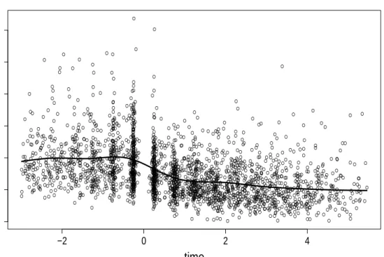
The data were collected within the Multicenter AIDS Cohort Study (MACS), which has fol-lowed nearly 5000 gay or bisexual men from Baltimore, Pittsburgh, Chicago and Los Angeles since 1984 (see Kaslow et al., 1987; Zeger and Diggle, 1994). The study includes 1809 men who were infected with HIV when the study began and another 371 men who were seronegative at entry and seroconverted during the followup. In our application 369 seroconverters with 2376 measurements over time are used. The interesting response variable is the number of CD4 cells by which progression of disease may be assessed. Covariates include years since seroconversion, packs of cigarettes a day, recreational drug use (yes/no), number of sexual partners, age and a mental illness score (cesd). The data has been already examined in Tutz and Reithinger (2007).
Since the forms of the effects are not known, time since seroconversion, age and the mental illness score may be considered as unspecified additive effects. We consider the semi-parametric mixed model with linear predictorg(µit) =ηit=ηparit +ηitadd+bi,whereµitdenotes the expected
CD4 number of cells for subjecti on measurement t (taken at irregular time intervals). The parametric and nonparametric terms are
ηpar
it =β0+ drugsitβ1+ partnersitβ2+ packsitβ3, ηaddit =α1(timeit) +α2(ageit) +α3(cesdit).
We fit an overdispersed Poisson model with natural link. The overdispersion parameter Φ is estimated by use of Pearson residuals ˆrit= (yit−µˆit)/(v(ˆµit))
1 2 as ˆ Φ = 1 N−df n X i=1 Ti X t=1 ˆ rit2, N = n X i=1 Ti, (15)
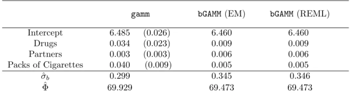
where the degrees of freedom (df) correspond to the trace of the hat-matrix. The results for the estimation of fixed effects, overdispersion parameter ˆΦ and ˆσbfor thegammfunction (Wood, 2006) and for thebGAMMalgorithm are given in Table 5.
gamm bGAMM(EM) bGAMM(REML)
Intercept 6.485 (0.026) 6.460 6.460 Drugs 0.034 (0.023) 0.009 0.009 Partners 0.003 (0.003) 0.006 0.006 Packs of Cigarettes 0.040 (0.009) 0.005 0.005 ˆ σb 0.299 0.345 0.346 ˆ Φ 69.929 69.473 69.473
Table 5: Estimates for the AIDS Cohort Study MACS with gammfunction (standard deviations in brackets) andbGAMMalgorithm
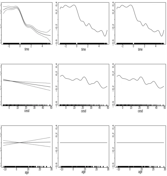
The main interest is in the typical time course of CD4 cell decay and the variability across subjects (see also Zeger and Diggle, 1994). Figure 6 shows the data together with an estimated overall smooth effect of time on CD4 cell decay derived by thegamm function. In Figure 7 the smooth effects of time, the mental illness score and age are given for bothgamm function and
bGAMM algorithm. It is seen that there is a decease in CD4 cells with time and with higher
values of the mental illness score. Thegammfunction estimates a very slight increase for age, while for thebGAMMalgorithm age is not selected and therefore has no effect at all.
5.2
The German Bundesliga
In the study the effect of team specific influence variables on the sportive success of the 18 soccer clubs of Germany’s first soccer division, the Bundesliga, has been investigated for the last three seasons 2007/2008 to 2009/2010. The response variable is the number of points, on which the league’s form table is based. Each team gets three points for wins, one point for every draw and no points for defeats. A brief description of the team specific covariates in the
● ● ● ● ● ● ● ● ● ● ● ● ● ● ● ● ● ● ● ● ● ● ● ● ● ● ● ● ● ● ● ● ● ● ● ● ● ● ● ● ● ● ● ● ● ● ● ● ● ● ● ● ● ● ● ● ● ● ● ● ● ● ● ● ● ● ● ● ● ● ● ● ● ● ● ● ● ● ● ● ● ● ● ● ● ● ● ● ● ● ● ● ● ● ● ● ● ● ● ● ● ● ● ● ● ● ● ● ● ● ● ● ● ● ● ● ● ● ● ● ● ● ● ● ● ● ● ● ● ● ● ● ● ● ● ● ● ● ● ● ● ● ● ● ● ● ● ● ● ● ● ● ● ● ● ● ● ● ● ● ● ● ● ● ● ● ● ● ● ● ● ● ● ● ● ● ● ● ● ● ● ● ● ● ● ● ● ● ● ● ● ● ● ● ● ● ● ● ● ● ● ● ● ● ● ● ● ● ● ● ● ● ● ● ● ● ● ● ● ● ● ● ● ● ● ● ● ● ● ● ● ● ● ● ● ● ● ● ● ● ● ● ● ● ● ● ● ● ● ● ● ● ● ● ● ● ● ● ● ● ● ● ● ● ● ● ● ● ● ● ● ● ● ● ● ● ● ● ● ● ● ● ● ● ● ● ● ● ● ● ● ● ● ● ● ● ● ● ● ● ● ● ● ● ● ● ● ● ● ● ● ● ● ● ● ● ● ● ● ● ● ● ● ● ● ● ● ● ● ● ● ● ● ● ● ● ● ● ● ● ● ● ● ● ● ● ● ● ● ● ● ● ● ● ● ● ● ● ● ● ● ● ● ● ● ● ● ● ● ● ● ● ● ● ● ● ● ● ● ● ● ● ● ● ● ● ● ● ● ● ● ● ● ● ● ● ● ● ● ● ● ● ● ● ● ● ● ● ● ● ● ● ● ● ● ● ● ● ● ● ● ● ● ● ● ● ● ● ● ● ● ● ● ● ● ● ● ● ● ● ● ● ● ● ● ● ● ● ● ● ● ● ● ● ● ● ● ● ● ● ● ● ● ● ● ● ● ● ● ● ● ● ● ● ● ● ● ● ● ● ● ● ● ● ● ● ● ● ● ● ● ● ● ● ● ● ● ● ● ● ● ● ● ● ● ● ● ● ● ● ● ● ● ● ● ● ● ● ● ● ● ● ● ● ● ● ● ● ● ● ● ● ● ● ● ● ● ● ● ● ● ● ● ● ● ● ● ● ● ● ● ● ● ● ● ● ● ● ● ● ● ● ● ● ● ● ● ● ● ● ● ● ● ● ● ● ● ● ● ● ● ● ● ● ● ● ● ● ● ● ● ● ● ● ● ● ● ● ● ● ● ● ● ● ● ● ● ● ● ● ● ● ● ● ● ● ● ● ● ● ● ● ● ● ● ● ● ● ● ● ● ● ● ● ● ● ● ● ● ● ● ● ● ● ● ● ● ● ● ● ● ● ● ● ● ● ● ● ● ● ● ● ● ● ● ● ● ● ● ● ● ● ● ● ● ● ● ● ● ● ● ● ● ● ● ● ● ● ● ● ● ● ● ● ● ● ● ● ● ● ● ● ● ● ● ● ● ● ● ● ● ● ● ● ● ● ● ● ● ● ● ● ● ● ● ● ● ● ● ● ● ● ● ● ● ● ● ● ● ● ● ● ● ● ● ● ● ● ● ● ● ● ● ● ● ● ● ● ● ● ● ● ● ● ● ● ● ● ● ● ● ● ● ● ● ● ● ● ● ● ● ● ● ● ● ● ● ● ● ● ● ● ● ● ● ● ● ● ● ● ● ● ● ● ● ● ● ● ● ● ● ● ● ● ● ● ● ● ● ● ● ● ● ● ● ● ● ● ● ● ● ● ● ● ● ● ● ● ● ● ● ● ● ● ● ● ● ● ● ● ● ● ● ● ● ● ● ● ● ● ● ● ● ● ● ● ● ● ● ● ● ● ● ● ● ● ● ● ● ● ● ● ● ● ● ● ● ● ● ● ● ● ● ● ● ● ● ● ● ● ● ● ● ● ● ● ● ● ● ● ● ● ● ● ● ● ● ● ● ● ● ● ● ● ● ● ● ● ● ● ● ● ● ● ● ● ● ● ● ● ● ● ● ● ● ● ● ● ● ● ● ● ● ● ● ● ● ● ● ● ● ● ● ● ● ● ● ● ● ● ● ● ● ● ● ● ● ● ● ● ● ● ● ● ● ● ● ● ● ● ● ● ● ● ● ● ● ● ● ● ● ● ● ● ● ● ● ● ● ● ● ● ● ● ● ● ● ● ● ● ● ● ● ● ● ● ● ● ● ● ● ● ● ● ● ● ● ● ● ● ● ● ● ● ● ● ● ● ● ● ● ● ● ● ● ● ● ● ● ● ● ● ● ● ● ● ● ● ● ● ● ● ● ● ● ● ● ● ● ● ● ● ● ● ● ● ● ● ● ● ● ● ● ● ● ● ● ● ● ● ● ● ● ● ● ● ● ● ● ● ● ● ● ● ● ● ● ● ● ● ● ● ● ● ● ● ● ● ● ● ● ● ● ● ● ● ● ● ● ● ● ● ● ● ● ● ● ● ● ● ● ● ● ● ● ● ● ● ● ● ● ● ● ● ● ● ● ● ● ● ● ● ● ● ● ● ● ● ● ● ● ● ● ● ● ● ● ● ● ● ● ● ● ● ● ● ● ● ● ● ● ● ● ● ● ● ● ● ● ● ● ● ● ● ● ● ● ● ● ● ● ● ● ● ● ● ● ● ● ● ● ● ● ● ● ● ● ● ● ● ● ● ● ● ● ● ● ● ● ● ● ● ● ● ● ● ● ● ● ● ● ● ● ● ● ● ● ● ● ● ● ● ● ● ● ● ● ● ● ● ● ● ● ● ● ● ● ● ● ● ● ● ● ● ● ● ● ● ● ● ● ● ● ● ● ● ● ● ● ● ● ● ● ● ● ● ● ● ● ● ● ● ● ● ● ● ● ● ● ● ● ● ● ● ● ● ● ● ● ● ● ● ● ● ● ● ● ● ● ● ● ● ● ● ● ● ● ● ● ● ● ● ● ● ● ● ● ● ● ● ● ● ● ● ● ● ● ● ● ● ● ● ● ● ● ● ● ● ● ● ● ● ● ● ● ● ● ● ● ● ● ● ● ● ● ● ● ● ● ● ● ● ● ● ● ● ● ● ● ● ● ● ● ● ● ● ● ● ● ● ● ● ● ● ● ● ● ● ● ● ● ● ● ● ● ● ● ● ● ● ● ● ● ● ● ● ● ● ● ● ● ● ● ● ● ● ● ● ● ● ● ● ● ● ● ● ● ● ● ● ● ● ● ● ● ● ● ● ● ● ● ● ● ● ● ● ● ● ● ● ● ● ● ● ● ● ● ● ● ● ● ● ● ● ● ● ● ● ● ● ● ● ● ● ● ● ● ● ● ● ● ● ● ● ● ● ● ● ● ● ● ● ● ● ● ● ● ● ● ● ● ● ● ● ● ● ● ● ● ● ● ● ● ● ● ● ● ● ● ● ● ● ● ● ● ● ● ● ● ● ● ● ● ● ● ● ● ● ● ● ● ● ● ● ● ● ● ● ● ● ● ● ● ● ● ● ● ● ● ● ● ● ● ● ● ● ● ● ● ● ● ● ● ● ● ● ● ● ● ● ● ● ● ● ● ● ● ● ● ● ● ● ● ● ● ● ● ● ● ● ● ● ● ● ● ● ● ● ● ● ● ● ● ● ● ● ● ● ● ● ● ● ● ● ● ● ● ● ● ● ● ● ● ● ● ● ● ● ● ● ● ● ● ● ● ● ● ● ● ● ● ● ● ● ● ● ● ● ● ● ● ● ● ● ● ● ● ● ● ● ● ● ● ● ● ● ● ● ● ● ● ● ● ● ● ● ● ● ● ● ● ● ● ● ● ● ● ● ● ● ● ● ● ● ● ● ● ● ● ● ● ● ● ● ● ● ● ● ● ● ● ● ● ● ● ● ● ● ● ● ● ● ● ● ● ● ● ● ● ● ● ● ● ● ● ● ● ● ● ● ● ● ● ● ● ● ● ● ● ● ● ● ● ● ● ● ● ● ● ● ● ● ● ● ● ● ● ● ● ● ● ● ● ● ● ● ● ● ● ● ● ● ● ● ● ● ● ● ● ● ● ● ● ● ● ● ● ● ● ● ● ● ● ● ● ● ● ● ● ● ● ● ● ● ● ● ● ● ● ● ● ● ● ● ● ● ● ● ● ● ● ● ● ● ● ● ● ● ● ● ● ● ● ● ● ● ● ● ● ● ● ● ● ● ● ● ● ● ● ● ● ● ● ● ● ● ● ● ● ● ● ● ● ● ● ● ● ● ● ● ● ● ● ● ● ● ● ● ● ● ● ● ● ● ● ● ● ● ● ● ● ● ● ● ● ● ● ● ● ● ● ● ● ● ● ● ● ● ● ● ● ● ● ● ● ● ● ● ● ● ● ● ● ● ● ● ● ● ● ● ● ● ● ● ● ● ● ● ● ● ● ● ● ● ● ● ● ● ● ● ● ● ● ● ● ● ● ● ● ● ● ● ● ● ● ● ● ● ● ● ● ● ● ● ● ● ● ● ● ● ● ● ● ● ● ● ● ● ● ● ● ● ● ● ● ● ● ● ● ● ● ● ● ● ● ● ● ● ● ● ● ● ● ● ● ● ● ● ● ● ● ● ● ● ● ● ● ● ● ● ● ● ● ● ● ● ● ● ● ● ● ● ● ● ● ● ● ● ● ● ● ● ● ● ● ● ● ● ● ● ● ● ● ● ● ● ● ● ● ● ● ● ● ● ● ● ● ● ● ● ● ● ● ● ● ● ● ● ● ● ● ● ● ● ● ● ● ● ● ● ● ● ● ● ● ● ● ● ● ● ● ● ● ● ● ● ● ● ● ● ● ● ● ● ● ● ● ● ● ● ● ● ● ● ● ● ● ● ● ● ● ● ● ● ● ● ● ● ● ● ● ● ● ● ● ● ● ● ● ● ● ● ● ● ● ● ● ● ● ● ● ● ● ● ● ● ● ● ● ● ● ● ● ● ● ● ● ● ● ● ● ● ● ● ● ● ● ● ● ● ● ● ● ● ● ● ● ● ● ● ● ● ● ● ● ● ● ● ● ● ● ● ● ● ● ● ● ● ● ● ● ● ● ● ● ● ● ● ● ● ● ● ● ● ● ● ● ● ● ● ● ● ● ● ● ● ● ● ● ● ● ● ● ● ● ● ● ● ● ● ● ● ● ● ● ● ● ● ● ● ● ● ● ● ● ● ● ● ● ● ● ● ● ● ● ● ● ● ● ● ● ● ● ● ● ● −2 0 2 4 0 500 1000 2000 3000
time
cd4Figure 6: Data from Multicenter AIDS Cohort Study (MACS) and smoothed time effect
data can be found in Table 6.
Covariate Description
ball possession average percentage of ball possession per game tackle average percentage of tackles won per game
unfairness average number of unfairness points per game (1 point for yellow card, 3 points for second yellow card, 5 points for red card)
transfer spendings money spent for new players during a season (in Euro)
transfer receipts money earned through player transfers during a season (in Euro) attendance average attendance during a season
sold out number of ticket sold outs during a season
Table 6: Description of covariates for the German Bundesliga data
Except for the variables“ball possession” and “tackles”, which were treated as parametric terms, for all other variables unspecified additive effects were considered. Due to the very dif-ferent ranges of values covariates have been standardized. The corresponding semi-parametric mixed model has the form
−2 0 2 4 −0.6 −0.2 0.2 0.4 time −2 0 2 4 −0.6 −0.2 0.2 0.4 time −2 0 2 4 −0.6 −0.2 0.2 0.4 time 0 10 20 30 40 50 −0.6 −0.2 0.2 0.4 cesd 0 10 20 30 40 50 −0.6 −0.2 0.2 0.4 cesd 0 10 20 30 40 50 −0.6 −0.2 0.2 0.4 cesd −10 0 10 20 30 −0.6 −0.2 0.2 0.4 age −10 0 10 20 30 −0.6 −0.2 0.2 0.4 age −10 0 10 20 30 −0.6 −0.2 0.2 0.4 age
Figure 7: Estimated smooth effect of time, age and cesd computed with thegammmodel (left), the
bGAMMEM model (middle) and thebGAMMREML model (right) for CD4 data
whereµitdenotes the expected number of points for soccer teamiin seasont. The parametric and nonparametric terms are
ηpar
it = β0+ ball possessionitβ1+ tacklesitβ2
ηadd
it = α1(transfer spendingit) +α2(transfer receiptsit) +α3(unfairnessit)
+α4(attendanceit) +α5(sold outit).
Again we fit an overdispersed Poisson model with natural link while the overdispersion param-eter Φ is estimated using (15).
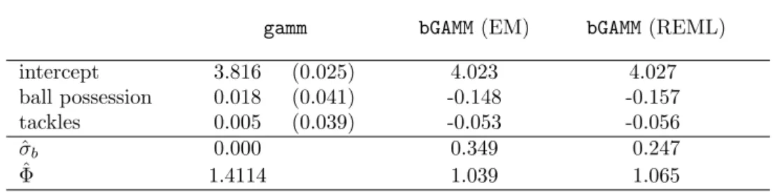
gammfunction and for thebGAMMalgorithm are given in Table 7. Both boosting functions
esti-gamm bGAMM(EM) bGAMM(REML)
intercept 3.816 (0.025) 4.023 4.027 ball possession 0.018 (0.041) -0.148 -0.157 tackles 0.005 (0.039) -0.053 -0.056 ˆ σb 0.000 0.349 0.247 ˆ Φ 1.4114 1.039 1.065
Table 7: Estimates for the German Bundesliga data with gamm function (standard deviations in brackets) andbGAMMalgorithm
mate dispersion parameters not far away from one, so that the Poisson model seems adequate. Thegammfunction provides a very low standard deviation (ˆσb=0.000014) of the random inter-cepts, while thebGAMMmodels lead to results that support the application of a random effects model, indicating that each soccer team has an individual bases level of points.
In Figure 8 the five smooth effects are presented. It becomes obvious, that all three ap-proaches estimate similar functions, but the two boosting apap-proaches exclude the variable “transfer receipts” from the model. Furthermore the smooth effect of the variable “transfer spendings” as well as the strongly positive effect of the variable “attendance” on the number of points are remarkable.
6
Concluding Remarks
Variable selection methods have been proposed that allow to extract the relevant predictors in generalized additive mixed models. The methods are shown to work in high-dimensional settings and turn out to be very stable. Performance suffers hardly when the number of noise variables grows.
Acknowledgement
The authors are grateful to Jasmin Abedieh for providing the German Bundesliga data, which were part of her bachelor thesis.
−1 0 1 2 3 4 −0.4 −0.2 0.0 0.2 0.4 transfer spendings −1 0 1 2 3 4 −0.4 −0.2 0.0 0.2 0.4 transfer spendings −1 0 1 2 3 4 −0.4 −0.2 0.0 0.2 0.4 transfer spendings 0 1 2 3 −0.4 −0.2 0.0 0.2 0.4 transfer receipts 0 1 2 3 −0.4 −0.2 0.0 0.2 0.4 transfer receipts 0 1 2 3 −0.4 −0.2 0.0 0.2 0.4 transfer receipts −2 −1 0 1 2 −0.4 −0.2 0.0 0.2 0.4 unfairness −2 −1 0 1 2 −0.4 −0.2 0.0 0.2 0.4 unfairness −2 −1 0 1 2 −0.4 −0.2 0.0 0.2 0.4 unfairness −1 0 1 2 −0.4 −0.2 0.0 0.2 0.4 attendance −1 0 1 2 −0.4 −0.2 0.0 0.2 0.4 attendance −1 0 1 2 −0.4 −0.2 0.0 0.2 0.4 attendance −1.0 −0.5 0.0 0.5 1.0 1.5 2.0 −0.4 −0.2 0.0 0.2 0.4 sold out −1.0 −0.5 0.0 0.5 1.0 1.5 2.0 −0.4 −0.2 0.0 0.2 0.4 sold out −1.0 −0.5 0.0 0.5 1.0 1.5 2.0 −0.4 −0.2 0.0 0.2 0.4 sold out
Appendix
A
Reparametrization of Penalized B-Splines
Suppose a functionf can be represented by akB-spline basis with functionsBi(x;d) of degree d, f(x) = k X i=1 αiBi(x;d), (16)
whereαi are unknown weight parameters. Let
f(xi) =Bααα, where B= B1(xi1;d) . . . Bk(xi1;d) .. . ... B1(xin;d) . . . Bk(xin;d) (17)
be the matrix of evaluated basis functions called B-spline design matrix. To control the roughness or “wiggliness” of the estimated function in (16) a penalty term is added to the log-likelihood, e.g. the common penaltyJ(ααα) =αααTKααα. We chooseK= (∆∆∆d)T∆∆∆d, where ∆∆∆d denotes the difference operator matrix of degreed, penalizing the differences between neighbor-ing coefficientsαiin order to avoid sudden “jumps” in the estimated function; see for example Whittaker (1923), Eilers (1995) or Eilers and Marx (1996) for the difference penalty. Fahrmeir et al. (2004) suggested a decomposition of the P-spline coefficients into an unpenalized part and a penalized part:
α α
α=Tααα0+Pαααp,
whereααα0 represents the unpenalized part andαααp the penalized part of the spline coefficient vector. For the construction of the matricesTandPone uses that the penalty matrixKcan be decomposed intoK= (∆∆∆d)T∆∆∆d,where ∆∆∆dhas full row rank (k
−d). Then the matrixPis given by
P= ∆∆∆d(∆∆∆d)T−1(∆∆∆d)T.
According to Green (1987) the requirements ∆∆∆dT = 0 and T∆∆∆d = 0 have to hold and the matrix [∆∆∆d,T] has to be nonsingular. As a consequence,Tis a (k
×d) matrix representing a basis of the nullspace ofK. For the difference penalty of degreedthe basis is straightforward, consisting of all monomials up to degreed−1 defined by the knots of the B-spline. With the B-spline design matrix from equation (17) one obtains.
and the penalty term simplifies to J(ααα) = αααTKααα=αααT(∆∆∆d)T∆∆∆dααα = (Tααα0+Pαααp)T(∆∆∆d)T∆∆∆d(Tααα0+Pαααp) = αααTpP T (∆∆∆d)T∆∆∆dPαααp=αααTpαααp.
Thus, all in all, with ˜αααT := (αααT
0, αααTp), ΦΦΦ := [Xu,Zp] and ˜K := Diag(0, . . . ,0,1, . . . ,1) being a diagonal matrix with zeros corresponding toααα0 and ones corresponding toαααp, one obtains
J(ααα) = ˜αααTK˜αα,α˜ andBααα= ΦΦΦ˜ααα.
B
Reparametrization in semiparametric models
In this section a small additional step to the reparametrization from Appendix A is explained, that becomes necessary if the model is semiparametric, with the parametric term containing the intercept. Notice that the (k×d)-matrixXu from Appendix A has the general form
Xu= 1 ξ1,1 . . . ξ1,d−1 1 ... ... .. . ... ... 1 ξk,1 . . . ξk,d−1 ,
where the first column with ones refers to the level of the function in (16). If the parametric term of the model already contains the intercept, the estimated functionf(x) must be centered around zero in order to avoid identification problems. This can be achieved by dropping the first column of the matrixXu. Then the dimensions of Xu and ΦΦΦ decrease to (n×(d−1)) and to (n×(k−1)), respectively. As a consequence the first value ofααα0, representing the level
of the estimated function, doesn’t have to be estimated anymore and also ˜αααdecreases by one dimension.
References
Breslow, N. E. and D. G. Clayton (1993). Approximate inference in generalized linear mixed model. Journal of the American Statistical Association 88, 9–25.
Breslow, N. E. and X. Lin (1995). Bias correction in generalized linear mixed models with a single component of dispersion. Biometrika 82, 81–91.
B¨uhlmann, P. and B. Yu (2003). Boosting with the L2 loss: Regression and classification.
Journal of the American Statistical Association 98, 324–339.
Eilers, P. H. C. (1995). Indirect observations, composite link models and penalized likelihood. In G. U. H. Seeber, B. J. Francis, R. Hatzinger, and G. Steckel-Berger (Eds.),Proceedings
of the 10th International Workshop on Statistical Modelling. New York: Springer.
Eilers, P. H. C. and B. D. Marx (1996). Flexible smoothing with B-splines and Penalties.
Statistical Science 11, 89–121.
Fahrmeir, L., T. Kneib, and S. Lang (2004). Penalized structured additive regression for space-time data: a Bayesian perspective. Statistica Sinica 14, 731–761.
Fahrmeir, L. and G. Tutz (2001). Multivariate Statistical Modelling Based on Generalized
Linear Models (2nd ed.). New York: Springer-Verlag.
Freund, Y. and R. E. Schapire (1996). Experiments with a new boosting algorithm. In
Pro-ceedings of the Thirteenth International Conference on Machine Learning, pp. 148–156. San
Francisco, CA: Morgan Kaufmann.
Friedman, J. H. (2001). Greedy function approximation: a gradient boosting machine. Annals
of Statistics 29, 337–407.
Friedman, J. H., T. Hastie, and R. Tibshirani (2000). Additive logistic regression: A statistical view of boosting. Annals of Statistics 28, 337–407.
Green, P. J. (1987). Penalized likelihood for general semi-parametric regression models.
Inter-national Statistical Review 55, 245–259.
Hastie, T. and R. Tibshirani (1990).Generalized Additive Models. London: Chapman & Hall. Kaslow, R. A., D. G. Ostrow, R. Detels, J. P. Phair, B. Polk, and C. R. Rinaldo (1987). The multicenter aids cohort study: rationale, organization and selected characteristic of the participants. American Journal of Epidemiology 126, 310–318.
Lin, X. and N. E. Breslow (1996). Bias correction in generalized linear mixed models with multiple components of dispersion. Journal of the American Statistical Association 91, 1007–1016.
Lin, X. and D. Zhang (1999). Inference in generalized additive mixed models by using smooth-ing splines. Journal of the Royal Statistical Society B61, 381–400.
Littell, R., G. Milliken, W. Stroup, and R. Wolfinger (1996). SAS System for Mixed Models. Cary, NC: SAS Institue Inc.
Marx, D. B. and P. H. C. Eilers (1998). Direct generalized additive modelling with penalized likelihood. Comp. Stat. & Data Analysis 28, 193–209.
Ruppert, D., M. P. Wand, and R. J. Carroll (2003). Semiparametric Regression. Cambridge: Cambridge University Press.
Tutz, G. and A. Groll (2011). Binary and Ordinal Random Effects Models Including Variable Selection. Journal of Computational and Graphical Statistics. Submitted.
Tutz, G. and W. Hennevogl (1996). Random effects in ordinal regression models. Comput.
Stat. & Data Analysis 22, 537–557.
Tutz, G. and F. Reithinger (2007). Flexible semiparametric mixed models. Statistics in
Medicine 26, 2872–2900.
Venables, W. N. and B. D. Ripley (2002).Modern Applied Statistics with S (Fourth ed.). New York: Springer.
Vonesh, E. F. (1996). A note on the use of laplace’s approximatio for nonlinear mixed-effects models. Biometrika 83, 447–452.
Wand, M. P. (2000). A comparison of regression spline smoothing procedures. Computational
Statistics 15, 443–462.
Whittaker, E. T. (1923). On a new method of graduation.Proc. Edinborough Math. Assoc. 78, 81–89.
Wolfinger, R. and M. O’Connell (1993). Generalized linear mixed models; a pseudolikelihood approach. Journal Statist. Comput. Simulation 48, 233–243.
Wood, S. N. (2004). Stable and efficient multiple smoothing parameter estimation for gener-alized additive models. Journal of the American Statistical Association 99.
Wood, S. N. (2006).Generalized Additive Models: An Introduction with R. London: Chapman & Hall.
Zeger, S. L. and P. J. Diggle (1994). Semi-parametric models for longitudinal data with application to CD4 cell numbers in HIV seroconverters. Biometrics 50, 689–699.
Zhang, D., X. Lin, J. Raz, and M. Sowers (1998). Semi-parametric stochastic mixed models for longitudinal data. jasa 93, 710–719.