Autocorrelation measures for the quadratic assignment problem

(1)

Contents lists available atSciVerse ScienceDirect

Applied Mathematics Letters

journal homepage:www.elsevier.com/locate/aml

Autocorrelation measures for the quadratic assignment problem

Francisco Chicano

∗

, Gabriel Luque, Enrique Alba

E.T.S. Ingeniería Informática, University of Málaga, Spain

a r t i c l e i n f o

Article history: Received 29 July 2010

Received in revised form 23 September 2011

Accepted 26 September 2011

Keywords: Fitness landscapes Elementary landscapes Quadratic assignment problem Autocorrelation coefficient Autocorrelation length

a b s t r a c t

In this article we provide an exact expression for computing the autocorrelation coefficient

ξand the autocorrelation lengthℓof any arbitrary instance of the Quadratic Assignment Problem (QAP) in polynomial time using its elementary landscape decomposition. We also provide empirical evidence of the autocorrelation length conjecture in QAP and compute the parametersξandℓfor the 137 instances of the QAPLIB. Our goal is to better characterize the difficulty of this important class of problems to ease the future definition of new optimization methods. Also, the advance that this represents helps to consolidate QAP as an interesting and now better understood problem.

1. Introduction

Alandscapefor a combinatorial optimization problem is a triple

(

X

,

N

,

f

)

, wheref

:

X

→

_Ris the objective function to

be minimized (or maximized) and theneighborhoodfunctionNmaps a solutionx

∈

Xto the set of neighboring solutions. If

y

∈

N

(

x

)

thenyis a neighbor ofx. There is a especial kind of landscape, called anelementary landscape, which is of particular

interest in present research due to its properties. They are characterized by theGrover’s wave equation[1]:

avg

{

f

(

y

)

}

y∈N(x)

=

f

(

x

)

+

k

d

(

f

−

f

(

x

))

(1)

where dis the size of the neighborhood,

|

N

(

x

)

|

, which we assume the same for all the solutions in the search space

(regular neighborhood),fis the average solution evaluation over the entire search space, andkis a characteristic

(problem-dependent) constant. A general landscape

(

X

,

N

,

f

)

cannot always be said to be elementary, but even in this case it

is possible to characterize the function f as a sum of elementary landscapes [2], called the elementary componentsof

the landscape.

The Quadratic Assignment Problem (QAP) is a well-known NP-hard combinatorial optimization problem that is at the

core of many real-world optimization problems [3]. A lot of research has been devoted to analyze and solve the QAP itself,

and in fact some other problems can be formulated as special cases of the QAP, e.g., the Traveling Salesman Problem (TSP).

LetPbe a set ofnfacilities andLa set ofnlocations. For each pair of locationsiandj, an arbitrary distance is specifiedrijand

for each pair of facilitiespandq, a flow is specified

w

pq. The QAP consists of assigning to each location inLone facility inPin

such a way that the total cost of the assignment is minimized. Each location can only contain one facility and all the facilities must be assigned to one location. For each pair of locations the cost is computed as the product of the distance between

∗_{Corresponding author.}

(2)

the locations and the flow associated to the facilities in the locations. The total cost is the sum of all the costs associated to

each pair of locations. One solution to this problem is a bijection betweenLandP, that is,x

:

L

→

Psuch thatxis bijective.

Without loss of generality, we can just assume thatL

=

P

= {

1

,

2

, . . . ,

n

}

and each solutionxis a permutation inSn, the set

permutations of

{

1

,

2

, . . . ,

n

}

. The cost function to be minimized can be formally defined as:

f

(

x

)

=

n



i,j=1

rij

w

x(i)x(j)

.

(2)

In [4,5] the authors analyzed the QAP from the point of view of landscapes theory [6] and they found the elementary

landscape decomposition of the problem using the methodology presented in [7], providing expressions for each elementary

component. In this paper we use the elementary decomposition of the previous work to compute the autocorrelation

length

ℓ

and the autocorrelation coefficient

ξ

of any QAP instance in polynomial time (Section2). We also present

in Section3 empirical evidence of the autocorrelation length conjecture [8], which links these values to the number

of local optima of a problem, and we numerically compute

ℓ

and

ξ

for the well-known public instances of the

QAPLIB [9].

2. Autocorrelation of QAP

Let us consider an infinite random walk

{

x0

,

x1

, . . .

}

on the solution space such thatxi+1

∈

N

(

xi

)

. Therandom walk

autocorrelation function r

:

_N

→

_Ris defined as [10]:

r

(

s

)

=

⟨

f

(

x_t

)

f

(

x_t+s

)

⟩

x0,t

− ⟨

f

(

xt

)

⟩

2x0,t

⟨

f

(

xt

)

2

⟩

x0,t

− ⟨

f

(

xt

)

⟩

2 x0,t (3)

where the subindices x0 and t indicate that the averages are computed over all the starting solutions x0 and along

the complete random walk. The autocorrelation coefficient

ξ

of a problem is a parameter proposed by Angel and

Zissimopoulos [11] that gives a measure of its ruggedness. It is defined afterr

(

s

)

by

ξ

=

(

1

−

r

(

1

))

−1_[₁₂_{]. Another measure}

of ruggedness is theautocorrelation length

ℓ

[13] whose definition is

ℓ

=



∞

s=0r

(

s

)

. The autocorrelation coefficient

ξ

for the

QAP was exactly computed by Angel and Zissimopoulos in [14]. However, recent results (see [4]) suggest that the expression

in [14] could be invalid for some instances of the QAP. Using the landscape decomposition of the QAP we provide here a

simple derivation for the expressions of

ξ

and

ℓ

. First, let us present (without proof) the results of [5] that are relevant to

our goal.

Proposition 1 (Decomposition of the QAP). For the swap neighborhood, the function f defined in(2)can be written as the sum of at most three elementary landscapes with constants k1

=

2n

,

k2

=

2

(

n

−

1

)

, and k3

=

n: f

=

fc1

+

fc2

+

fc3. The elementary

components can be defined as

fc1

=

n



i,j,p,q=1 i̸=j,p̸=q

ψ

ijpq Ω1 (i,j),(p,q) 2n (4) fc2

=

n



i,j,p,q=1 i̸=j,p̸=q

ψ

ijpq Ω2 (i,j),(p,q) 2

(

n

−

2

)

(5) fc3

=

n



i,j,p,q=1 i̸=j,p̸=q

ψ

ijpq Ω3 (i,j),(p,q) n

(

n

−

2

)

+

n



i,p=1

ψ

iipp

ϕ

(i,i),(p,p) (6)

where

ψ

ijpq

=

rij

w

pq

, ϕ

(i,i),(p,p)is the function defined using Kronecker’s delta by

ϕ

(i,i),(p,p)

(

x

)

=

δ

p

x(i), and theΩfunctions are

particular cases of the parameterized

φ

functions defined as:

φ

(i,j),(p,q)α,β,γ ,ε,ζ

(

x

)

=











α

if x

(

i

)

=

p

∧

x

(

j

)

=

q

β

if x

(

i

)

=

q

∧

x

(

j

)

=

p

γ

if x

(

i

)

=

p

⊕

x

(

j

)

=

q

ε

if x

(

i

)

=

q

⊕

x

(

j

)

=

p

ζ

if x

(

i

)

̸=

p

,

q

∧

x

(

j

)

̸=

p

,

q

.

(7)

The definition of theΩ functions is as follows:Ω1

(i,j),(p,q)

=

φ

(i,j),(p,q)n−3,1−n,−2,0,−1,Ω(i,j),(p,q)2

=

φ

(i,j),(p,q)n−3,n−3,0,0,1, andΩ(i,j),(p,q)3

=

φ

2n−3,1,n−2,0,−1 (i,j),(p,q) .

(3)

Proposition 2 (Autocorrelation Measures). The autocorrelation coefficient

ξ

, the autocorrelation length

ℓ

, and the autocorrela-tion funcautocorrela-tion r

(

s

)

can be computed from the actual problem data (instance) using the expressions:

ξ

=



W1 4 n

−

1

+

W2 4 n

+

W3 2 n

−

1



−1

=

n

(

n

−

1

)

2n

(

1

+

W1

)

+

2W2

(

n

−

2

)

(8)

ℓ

=

d



W1 2n

+

W2 2

(

n

−

1

)

+

W3 n



=

W1

(

1

−

n

)

+

W2

(

2

−

n

)

+

2

(

n

−

1

)

4 (9) r

(

s

)

=

W1



1

−

4 n

−

1



s

+

W2



1

−

4 n



s

+

W3



1

−

2 n

−

1



s (10)

where the coefficients Wifor i

=

1

,

2

,

3are defined by

Wi

=

f_ci2

−

fci 2

f2

₋

_f2

.

(11)

Proof. A proof for(8)and(11)can be found in [5]. Eq.(9)is justified in [13] and(10)is proven in [2]. We also used the fact

thatW1

+

W2

+

W3

=

1 to removeW3in the expressions for

ξ

and

ℓ

.

As a consequence, we only need to computeW1 and W2 to obtain

ξ

and

ℓ

. Thus, we provide in this paper some

propositions that allow us to efficiently computeW1andW2. According to(11)we need to computef2

,

f

2 ,f_c2₁

,

fc1 2

,

f_c2₂, andfc2 2

. Let us start withfc1andfc2.

Proposition 3. Two expressions for fc1and fc2are:

fc1

= −

rt

w

t 2n (12) fc2

=

rt

w

t

(

n

−

3

)

2

(

n

−

1

)(

n

−

2

)

,

(13)

where rtand

w

tare defined as:

rt

=

n



i,j=1 i̸=j rij

;

w

t

=

n



p,q=1 p̸=q

w

pq

.

(14)

Proof. The average value ofΩ1_and_Ω2_is_Ω1

_{= −}

_{1, and}_Ω2

₌

(

_n

₋

₃

)/(

_n

₋

₁

)

_[₄_{]. Using these average values we can}

computefc1andfc2with the help of(4)and(5)as:

fc1

=

−

1 2n n



i,j,p,q=1 i̸=j,p̸=q

ψ

ijpq

;

fc2

=

n

−

3 2

(

n

−

1

)(

n

−

2

)

n



i,j,p,q=1 i̸=j,p̸=q

ψ

ijpq

.

(15)

Taking into account that

ψ

ijpq

=

rij

w

pqand using the notationrt

, w

t defined above we can transform(15)in(12)and

(13).

Both expressions(12)and(13)can be computed inO

(

n2

)

. Before giving an expression forf let us first introduce a new

functiontndefined as:

tn

:

P

(

{

1

, . . . ,

n

}

2

)

→

N Q

→

tn

(

Q

)

=



x∈Sn



(i,p)∈Q

δ

p x(i)

.

(16)

This function will be useful later in the computation off

,

f2

,

_f2

c1, andf 2

c2. According to its definition, the evaluation oftn

is not efficient since it requires a summation over all the permutations inSn. However, we can simplify the expression oftn

to make the computation more efficient as the following proposition states. Proposition 4. The function tnsatisfies the following equality:

tn

(

Q

)

=



(

n

− |

Q

|

)

!

if

|

Q1

| = |

Q2

| = |

Q

|

0 otherwise

,

(17)

(4)

Proof. The functiontnis, in fact, a counting function that is counting the number of elements inSnthat fulfill the condition



(i,p)∈Qx

(

i

)

=

p. Now, we must observe that if we find two pairs

(

i

,

p

)

and

(

j

,

q

)

inQ such thati

=

jandp

̸=

q, then the

value oftn

(

Q

)

must be zero because it is not possible to satisfy at the same timex

(

i

)

=

pandx

(

j

)

=

q. We can characterize

this situation using the condition

|

Q1

| ̸= |

Q

|

. That is, if the number of pairs inQis not equal to the number of first elements

of these pairs, then there exist inQ at least two pairs of the form

(

i

,

p

)

and (i

,

q) withp

̸=

qandtn

(

Q

)

=

0. For the same

reason,t

(

Q

)

=

0 if

|

Q2

| ̸= |

Q

|

. If

|

Q

| = |

Q1

| = |

Q2

|

then the pairs inQ fix the value for

|

Q

|

components of the solution

vector and the number of solutions inSnwith the fixed components istn

(

Q

)

=

(

n

− |

Q

|

)

!

.

Once we have defined thetnfunction and we know an efficient way of computing it we can provide an expression forf.

Proposition 5. An expression for f is:

f

=

rt

w

t n

(

n

−

1

)

+

rd

w

d n (18) where rd

=



n i=1riiand

w

d

=



n p=1

w

pp.

Proof. Using the definition offandtnwe can write:

f

=

1

|

Sn

|

n



i,j,p,q=1

ψ

ijpq





x∈Sn

δ

p x(i)

δ

qx(j)



=

1 n

!

n



i,j,p,q=1

ψ

ijpqtn

(

{

(

i

,

p

), (

j

,

q

)

}

).

(19)

If we take into account thattncan only take two different values, we can rewrite the previous expression as:

f

=

(

n

−

2

)

!

n

!

n



i,j,p,q=1 i̸=j,p̸=q

ψ

ijpq

+

(

n

−

1

)

!

n

!

n



i,p=1

ψ

iipp

=

rt

w

t n

(

n

−

1

)

+

rd

w

d n

.

(20)

With the help of the functiontnwe can also provide an expression forf2.

Proposition 6. An expression for f2_is:

f2

₌

1 n

!

n



i,j,p,q=1 n



i′_,j′_,p′_,q′₌₁

ψ

ijpq

ψ

i′_j′_p′_q′t_n



{

(

i

,

p

), (

j

,

q

), (

i′

,

p′

), (

j′

,

q′

)

}



(21)

which can be computed in O

(

n8

)

.

Proof. Using the definition offwe can write:

f2

₌

1

|

Sn

|



x∈Sn



_n



i,j,p,q=1

ψ

ijpq

δ

px(i)

δ

qx(j)



2

=

1 n

!



x∈Sn n



i,j,p,q=1 n



i′_,j′_,p′_,q′₌₁

ψ

ijpq

ψ

i′_j′_p′_q′

δ

p x(i)

δ

qx(j)

δ

p ′ x(i′₎

δ

q′ x(j′₎ (22)

which can be transformed into(21)by commuting the sums and using the definition oftn.

The computation off_c2₁

,

f_c2₂requires a more complex treatment. We present their expressions in the following

Proposition 7. Two expressions for f_c2₁and f_c2₂are:

f_c2₁

=

1 4n2

_·

_n

_!

n



i,j,p,q=1 i̸=j,p̸=q n



i′,j′,p′,q′ =1 i′ ̸=j′_,p′ ̸=q′

ψ

ijpq

ψ

i′_j′_p′_q′



₇



m=1 7



m′₌₁ c_mΩ1c_mΩ′1tn



v

i,j,p,q m

∪

v

i′,j′,p′,q′ m′





(23) f2 c2

=

1 4

(

n

−

2

)

2

_·

_n

_!

n



i,j,p,q=1 i̸=j,p̸=q n



i′_,j′_,p′_,q′ =1 i′ ̸=j′_,p′ ̸=q′

ψ

ijpq

ψ

i′_j′_p′_q′



₇



m=1 7



m′₌₁ c_mΩ2c_mΩ′2tn



v

i,j,p,q m

∪

v

i′,j′,p′,q′ m′





(24)

where the 7-dimensional parameterized vectors

v

∈

(

P

(

N2

))

7and c

∈

R7are given inTable1and cΩ

1

and cΩ2 denote the c vectors whose parameters

α, β, γ , ε, ζ

are those of Ω1 _and_Ω2_{, respectively, that is, c}Ω1

₌

_cn−3,1−n,−2,0,−1_{and c}Ω2

₌

(5)

Table 1

Content of the vectorsvi,j,p,q_and_cα,β,γ ,ε,ζ_.

Component (m) vi,j,p,q _cα,β,γ ,ε,ζ 1 ∅ ζ 2 {(i,p)} (γ−ζ) 3 {(i,q)} (ε−ζ ) 4 {(j,q)} (γ−ζ) 5 {(j,p)} (ε−ζ ) 6 {(i,p), (j,q)} (α−2γ+ζ) 7 {(i,q), (j,p)} (β−2ε+ζ)

Proof. After the definition offc1andfc2we can write:

f_c2₁

=

1 4n2

_·

_n

_!

n



i,j,p,q=1 i̸=j,p̸=q n



i′,j′,p′,q′ =1 i′ ̸=j′_,p′ ̸=q′

ψ

ijpq

ψ

i′_j′_p′_q′





x∈Sn Ω1 (i,j),(p,q)

(

x

)

Ω(i1′_,j′_),(p′_,q′₎

(

x

)



(25) f2 c2

=

1 4

(

n

−

2

)

2

_·

_n

_!

n



i,j,p,q=1 i̸=j,p̸=q n



i′_,j′_,p′_,q′ =1 i′ ̸=j′_,p′ ̸=q′

ψ

ijpq

ψ

i′_j′_p′_q′





x∈Sn Ω2 (i,j),(p,q)

(

x

)

Ω(i2′_,j′_),(p′_,q′₎

(

x

)



.

(26)

In this case it is not so simple to write the inner summation as a function oftn. We will write theΩfunctions as linear

combinations of Kronecker’s deltas using the definition of theΩ functions and the following characterization of the

φ

functions, which can be easily obtained after(7):

φ

(i,j),(p,q)α,β,γ ,ε,ζ

(

x

)

=

αδ

x(i)p

δ

x(j)q

+

βδ

x(i)q

δ

x(j)p

+

γ (δ

x(i)p

−

δ

qx(j)

)

2

+

ε(δ

_xq₍_i₎

−

δ

_xp₍_j₎

)

2

+

ζ (

1

−

δ

_xp₍_i₎

)(

1

−

δ

q_x₍_i₎

)(

1

−

δ

_xp₍_j₎

)(

1

−

δ

_xq₍_j₎

)

=

(γ

−

ζ )(δ

p_x₍_i₎

+

δ

_xq₍_j₎

)

+

(ε

−

ζ )(δ

_xq₍_i₎

+

δ

p_x₍_j₎

)

+

δ

_xp₍_i₎

δ

_xq₍_j₎

(α

−

2

γ

+

ζ )

+

δ

_xq₍_i₎

δ

_xp₍_j₎

(β

−

2

ε

+

ζ )

+

ζ .

(27)

Thus,

φ

_(i,j),(p,q)α,β,γ ,ε,ζis a sum of six terms with

δ

and one constant, and the summation



x∈Sn

φ

α,β,γ ,ε,ζ(i,j),(p,q)

(

x

)φ

(iα,β,γ ,ε,ζ′_,j′_),(p′_,q′₎

(

x

)

(28)

can be written as a weighted sum of 49tnterms. In order to write this summation in a compact way we define one vector

denoted with

v

i,j,p,qcontaining the sets to be considered in thetnterms and a vectorcα,β,γ ,ε,ζcontaining the coefficients

for thetnterms. The content of the previous vectors is shown inTable 1. Using

v

andcwe can write the summation of the

product of

φ

functions in the following way:



x∈Sn

φ

α,β,γ ,ε,ζ(i,j),(p,q)

(

x

)φ

(α,β,γ ,ε,ζi′_,_j′_),(_p′_,_q′₎

(

x

)

=

7



m=1 7



m′₌₁ c_mα,β,γ ,ε,ζc_mα,β,γ ,ε,ζ′ tn



v

i,j,p,q m

∪

v

i′,j′,p′,q′ m′



(29)

and using the previous equality in(25)and(26)we obtain(23)and(24).

Now we have efficient expressions for computingf

,

f2

,

_f

c1

,

fc21,fc2, andfc22. With these expressions we are in conditions

enabling us to efficiently compute the autocorrelation measures

ξ

and

ℓ

. This result is summarized in the following

Theorem 1 (Efficient Computation of

ξ

and

ℓ

).In the QAP, the values of

ξ

and

ℓ

related to the swap neighborhood and defined by

ξ

=

n

(

n

−

1

)

2n

(

1

+

W1

)

+

2W2

(

n

−

2

)

(8)

ℓ

=

W1

(

1

−

n

)

+

W2

(

2

−

n

)

+

2

(

n

−

1

)

4 (9)

can be computed in polynomial time over the size of the problem n using Eqs.(12),(13),(18),(21),(23)and(24).

Proof. After computingf

,

fc1

,

fc2

,

f2

,

fc21, andfc22using the Eqs.(12),(13),(18),(21),(23)and(24)we should computeW1

andW2using Eq.(11). Then, the autocorrelation coefficient

ξ

can be obtained with(8)and

ℓ

can be computed with(9). None

of the previous equations requires more than eight nested summations overnand, thus, the computation can be done in

O

(

n8

₎

_.

(6)

Table 2

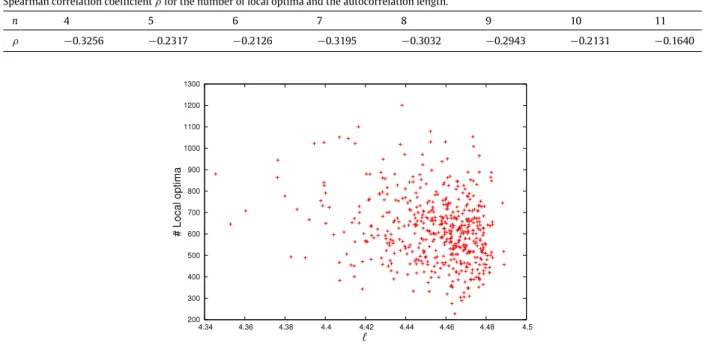
Spearman correlation coefficientρfor the number of local optima and the autocorrelation length.

n 4 5 6 7 8 9 10 11

ρ −0.3256 −0.2317 −0.2126 −0.3195 −0.3032 −0.2943 −0.2131 −0.1640

Fig. 1. Number of local optima against the autocorrelation lengthℓfor random instances of QAP withn=10.

We have gone one step further and we have expanded the expressions forf2

_,

_f2

c1, andf 2

c2in order to make a more efficient

computation. The result is aO

(

n2

₎

_{algorithm (which we omit due to space constraints) to compute}

_ℓ

_and

_ξ

_{. It is not difficult}

to prove that such an algorithm is optimal in complexity, since the data of a QAP instance is composed of 2n2_{numbers which}

have to be taken into account in order to compute the autocorrelation measures. 3. Autocorrelation length conjecture

The autocorrelation length is specially important in optimization because of theautocorrelation length conjecture, which

claims that in many landscapes the number of local optimaMcan be estimated by the expressionM

≈

_|_X(x|X|

0,ℓ)|[8], where

X

(

x0

, ℓ)

is the set of solutions reachable fromx0in

ℓ

(the autocorrelation length) or less local movements (jumps between

neighbors). The previous expression is not an equation, but an approximation. It can be useful to compare the estimated number of local optima in two instances of the same problem. In effect, for a given problem in which the conjecture is

applicable, the higher the value of

ℓ

(or

ξ

) the lower the number of local optima. In a landscape with a low number of local

optima, a local search strategy cana priorifind the global optimum using fewer steps. This phenomenon has been empirically

observed for the Quadratic Assignment Problem (QAP) by Angel and Zissimopoulos in [14].

In order to check the autocorrelation length conjecture in the QAP we have generated 4000 random instances of QAP

with sizes varying betweenn

=

4 andn

=

11 (500 for each value ofn) using a random generator where the elements of the

matrices are uniformly selected from the range [0,99]. For each instance we computed the autocorrelation length

ℓ

using

(9)and the number of local optima (minima) by complete enumeration of the search space. We computed the Spearman

correlation coefficient

ρ

of the number of local optima and

ℓ

for the instances of the same size. The results are shown in

Table 2. We can observe an inverse correlation (around

−

0

.

3) between the number of local optima and the autocorrelation length. Although this fact is in agreement with the autocorrelation length conjecture, the correlation coefficient is low.

However, Angel and Zissimopoulos [14] used a simulated annealing algorithm based on the swap neighborhood and reported

a better performance of the algorithm as the autocorrelation length increased. Assuming that the number of local optima is a parameter with an important influence on the search, we conclude that even in problems in which the number of

local optima is lowly correlated with

ℓ

(like QAP) the autocorrelation measures (

ξ

and

ℓ

) can be useful as estimators of the

performance of local search algorithms.

InFig. 1we plot the number of local optima against the autocorrelation length

ℓ

for all the instances of sizen

=

10. We can observe a slight trend: as the autocorrelation length increases the number of local optima decreases. The trend is the same in all the instances with different sizes (we omit their plots).

In a second experiment we check that the autocorrelation measures provided by the elementary landscape decomposition are the same as the ones computed using statistical methods. For this experiment we have chosen six

instances of the QAPLIB [9]: two small, two medium and two large instances. For each instance we have generated one

(7)

Table 3

Experimental (E) and exact (T) values for the autocorrelation functionr(s)in six instances of the QAPLIB (sfrom 1 to 6).

Instances r(1) r(2) r(3) r(4) r(5) r(6) tai10a E 0.624255 0.393489 0.250810 0.161890 0.106102 0.070590 T 0.624380 0.393590 0.250903 0.162013 0.106129 0.070617 esc16a E 0.749984 0.562424 0.421759 0.316365 0.237300 0.177939 T 0.750000 0.562500 0.421875 0.316406 0.237305 0.177979 esc64a E 0.937402 0.878700 0.823668 0.772063 0.723672 0.678292 T 0.937500 0.878906 0.823975 0.772476 0.724196 0.678934 lipa70a E 0.943369 0.890041 0.839723 0.792267 0.747507 0.705296 T 0.943479 0.890170 0.839890 0.792466 0.747735 0.705545 tho150 E 0.975680 0.951974 0.928863 0.906338 0.884384 0.862981 T 0.975722 0.952060 0.928997 0.906518 0.884607 0.863251 tai256c E 0.984364 0.968983 0.953843 0.938935 0.924256 0.909805 T 0.984375 0.968994 0.953854 0.938950 0.924279 0.909837 Table 4

Autocorrelation coefficientξand autocorrelation lengthℓfor the 137 instances of the QAPLIB.

Instance ξ ℓ Instance ξ ℓ Instance ξ ℓ Instance ξ ℓ bur26a 11.825 12.130 esc32b 8.000 8.000 nug16a 4.475 4.796 tai100b 35.472 39.613 bur26b 11.727 12.073 esc32c 8.000 8.000 nug16b 4.472 4.792 tai10a 2.662 2.774 bur26c 12.109 12.291 esc32d 8.000 8.000 nug17 4.836 5.220 tai10b 3.002 3.253 bur26d 12.050 12.258 esc32e 8.000 8.000 nug18 5.111 5.516 tai12a 3.419 3.674 bur26e 12.032 12.248 esc32f 8.000 8.000 nug20 5.800 6.311 tai12b 3.358 3.586 bur26f 11.962 12.208 esc32g 8.000 8.000 nug21 6.218 6.807 tai150b 40.458 42.947 bur26g 12.323 12.407 esc32h 8.000 8.000 nug22 6.751 7.446 tai15a 3.858 3.946 bur26h 12.296 12.392 esc64a 16.000 16.000 nug24 7.067 7.737 tai15b 7.000 7.000 chr12a 3.096 3.171 had12 3.743 4.092 nug25 7.308 7.987 tai17a 4.402 4.526 chr12b 3.201 3.346 had14 4.319 4.732 nug27 8.023 8.813 tai20a 5.211 5.385 chr12c 3.044 3.079 had16 4.405 4.690 nug28 8.181 8.949 tai20b 6.866 7.582 chr15a 3.917 4.049 had18 5.084 5.477 nug30 8.613 9.373 tai256c 64.000 64.000 chr15b 4.126 4.388 had20 5.830 6.352 rou12 3.158 3.275 tai25a 6.373 6.482 chr15c 3.843 3.920 kra30a 9.131 10.089 rou15 3.927 4.066 tai25b 6.896 7.374 chr18a 4.585 4.658 kra30b 9.086 10.031 rou20 5.354 5.628 tai30a 7.779 8.021 chr18b 4.632 4.742 kra32 9.848 10.908 scr12 3.407 3.657 tai30b 7.599 7.689 chr20a 5.105 5.195 lipa20a 5.072 5.135 scr15 4.303 4.650 tai35a 8.922 9.077 chr20b 5.035 5.067 lipa20b 5.196 5.358 scr20 5.514 5.885 tai35b 9.382 9.895 chr20c 5.260 5.469 lipa30a 7.622 7.732 sko100a 27.800 29.985 tai40a 10.216 10.413 chr22a 5.763 5.980 lipa30b 7.652 7.787 sko100b 28.106 30.470 tai40b 10.583 11.074 chr22b 5.672 5.819 lipa40a 10.154 10.295 sko100c 27.548 29.578 tai50a 12.675 12.839 chr25a 6.490 6.693 lipa40b 10.355 10.669 sko100d 27.535 29.557 tai50b 12.824 13.119 els19 5.178 5.494 lipa50a 12.684 12.855 sko100e 27.600 29.663 tai60a 15.292 15.563 esc128 32.000 32.000 lipa50b 12.854 13.174 sko100f 27.346 29.247 tai60b 17.837 19.691 esc16a 4.000 4.000 lipa60a 15.111 15.217 sko42 11.559 12.378 tai64c 16.000 16.000 esc16b 4.000 4.000 lipa60b 15.124 15.243 sko49 13.413 14.331 tai80a 20.214 20.419 esc16c 4.000 4.000 lipa70a 17.693 17.876 sko56 15.598 16.817 tai80b 24.021 26.612 esc16d 4.000 4.000 lipa70b 17.785 18.052 sko64 17.504 18.706 tho150 41.190 44.174 esc16e 4.000 4.000 lipa80a 20.102 20.201 sko72 19.929 21.436 tho30 8.326 8.938 esc16f – – lipa80b 20.191 20.373 sko81 22.739 24.629 tho40 11.492 12.531 esc16g 4.000 4.000 lipa90a 22.610 22.716 sko90 25.046 27.024 wil100 28.362 30.868 esc16h 4.000 4.000 lipa90b 22.733 22.957 ste36a 10.954 12.122 wil50 13.832 14.860 esc16i 4.000 4.000 nug12 3.135 3.237 ste36b 11.821 13.177

esc16j 4.000 4.000 nug14 3.892 4.155 ste36c 11.270 12.525 esc32a 8.000 8.000 nug15 4.029 4.234 tai100a 25.195 25.383

times and we have computed the average value for the 100 independent runs. The results empirically obtained and those

theoretically predicted with(10)can be found inTable 3(only fors

∈ [

1

,

6

]

). We can observe a great matching between

the empirical and the theoretical value, as expected. The advantage of the theoretical approach is that it is much faster. The

experimental results ofTable 3were obtained after 157 783 s of computation (more than 43 h). However, the exact values

were obtained evaluating Eq.(10)in 0.4 s, nearly half a million times faster.

Finally, we have computed the values of

ξ

and

ℓ

for the 137 QAP instances found in the QAPLIB database [9]. The results,

shown inTable 4in alphabetical order, could be helpful for future investigations on the QAP. In the table we can observe

some interesting behaviors, like that of the

esc

instances, which have always a value ofn

/

4 for

ξ

and

ℓ

. This happens

because in those instancesW1

=

W3

=

0 andW2

=

1, that is, they are elementary landscapes withk

=

2

(

n

−

1

)

. All the

elementary landscapes have a value for the autocorrelation measures that does not depend on the instance data, but only

on the problem size. In the case of

esc16f

, the objective function is a constant, that is, it takes the same value for every

(8)

We should also notice that the value of

ℓ

and

ξ

depend onn, the size of the problem instance. In effect, the values are bounded (see [4]) by n

−

1 4

≤

ξ,

ℓ

≤

n

−

1 2

.

(30)

Thus, the values of

ξ

and

ℓ

usually increase with the problem sizen. As a consequence, the autocorrelation length

conjecture can be applied only when the comparison is performed over instances with the same sizenand, in general,

it is not true that the higher the value of

ℓ

the easier to solve the instance, since the largest instances are usually the most

difficult ones and have the highest value for

ℓ

(and

ξ

). A good indicator of the difficulty of an instance could be the pair (n

, ℓ

).

4. Conclusions

In this article we give an optimal way of exactly computing the autocorrelation measures

ξ

and

ℓ

for the QAP. These two

parameters are important to better characterize QAP and to guide practitioners in the relative difficulty of the existing problem instances. These results can be automatically applied to all the subproblems of QAP, like de TSP. The main contributions of this work are:

•

An exact expression for computing the autocorrelation coefficient

ξ

and the autocorrelation length

ℓ

of the QAP in

polynomial time.

•

Empirical evidence of the autocorrelation length conjecture in practice for the QAP, by using arbitrarily generated

instances.

•

The numerical value of

ξ

and

ℓ

for all the instances in the QAPLIB database.

As a future work we plan to obtain exact expressions for the autocorrelation measures in other problems, and study the actual practical applications of the information obtained from them.

Acknowledgments

This work has been partially funded by the Spanish Ministry of Science and Innovation and FEDER under contract

TIN2008-06491-C04-01 (M∗_{project) and the Andalusian Government under contract P07-TIC-03044 (DIRICOM project).}

References

[1] L.K. Grover, Local search and the local structure of NP-complete problems, Operations Research Letters 12 (1992) 235–243. [2] P.F. Stadler, Landscapes and their correlation functions, Journal of Mathematical Chemistry 20 (1996) 1–45.

[3] M.R. Garey, D.S. Johnson, Computers and Intractability: A Guide to the Theory of NP-Completeness, W.H. Freeman, 1979.

[4] F. Chicano, G. Luque, E. Alba, Elementary landscapes decomposition of the quadratic assignment problem, in: Proceedings of GECCO 2010, ACM, Portland, OR, USA, 2010, pp. 1425–1432.

[5] F. Chicano, G. Luque, E. Alba, Elementary components of the quadratic assignment problem,arXiv:1109.4875v1, available from:http://arxiv.org (September 2011).

[6] J. Barnes, B. Dimova, S. Dokov, A. Solomon, The theory of elementary landscapes, Applied Mathematics Letters 16 (3) (2003) 337–343.

[7] F. Chicano, L.D. Whitley, E. Alba, A methodology to find the elementary landscape decomposition of combinatorial optimization problems, Evolutionary Computation Journal 19 (4) (2011).

[8] P.F. Stadler, Biological Evolution and Statistical Physics, Springer, 2002 (Chapter) Fitness Landscapes, pp. 183–204.

[9] R. Burkard, S. Karisch, F. Rendl, QAPLIB-a quadratic assignment problem library, Journal of Global Optimization 10 (1997) 391–403. [10] E. Weinberger, Correlated and uncorrelated fitness landscapes and how to tell the difference, Biological Cybernetics 63 (5) (1990) 325–336. [11] E. Angel, V. Zissimopoulos, Autocorrelation coefficient for the graph bipartitioning problem, Theoretical Computer Science 191 (1998) 229–243. [12] E. Angel, V. Zissimopoulos, On the classification of NP-complete problems in terms of their correlation coefficient, Discrete Applied Mathematics 99

(2000) 261–277.

[13] R. García-Pelayo, P. Stadler, Correlation length, isotropy and meta-stable states, Physica D: Nonlinear Phenomena 107 (2–4) (1997) 240–254. [14] E. Angel, V. Zissimopoulos, On the landscape ruggedness of the quadratic assignment problem, Theoretical Computer Science 263 (2000) 159–172.