Working PaPer SerieS
no 966 / november 2008
Large bayeSian vars
W O R K I N G PA P E R S E R I E S
N O 9 6 6 / N O V E M B E R 2 0 0 8
In 2008 all ECB publications feature a motif taken from the 10 banknote.
LARGE BAYESIAN VARs
1by Marta Bańbura
2, Domenico Giannone
3and Lucrezia Reichlin
4This paper can be downloaded without charge from http://www.ecb.europa.eu or from the Social Science Research Network electronic library at http://ssrn.com/abstract_id=1292332.
1 We would like to thank Simon Price, Barbara Rossi, Bob Rasche and Shaun Vahey and seminar participants at the New York Fed, the Cleveland Fed, the Chicago Fed, the ECB, the Bank of England, Queen Mary University, University of Rome Tor Vergata, Universitat Autμonoma de
© European Central Bank, 2008
Address
Kaiserstrasse 29
60311 Frankfurt am Main, Germany
Postal address
Postfach 16 03 19
60066 Frankfurt am Main, Germany
Telephone +49 69 1344 0 Website http://www.ecb.europa.eu Fax +49 69 1344 6000 All rights reserved.
Any reproduction, publication and reprint in the form of a different publication, whether printed or produced electronically, in whole or in part, is permitted only with the explicit written authorisation of the ECB or the author(s).
The views expressed in this paper do not necessarily refl ect those of the European Central Bank.
The statement of purpose for the ECB Working Paper Series is available from
Abstract 4
Non-technical summary 5
1 Introduction 7
2 Setting the priors for the VAR 10
2.1 Data 13
3 Forecast evaluation 14
3.1 Parsimony by lags selection 17
3.2 The Bayesian VAR and the Factor
Augmented VAR (FAVAR) 17
3.3 Prior on the sum of coeffi cients 20
4 Structural analysis: impulse response functions
and variance decomposition 21
5 Summary 26
References 27
European Central Bank Working Paper Series 40
Abstract
This paper shows that Vector Autoregression with Bayesian shrinkage is an appropriate tool for large dynamic models. We build on the results by De Mol, Giannone, and Reichlin (2008) and show that, when the degree of shrinkage is set in relation to the cross-sectional dimension, the forecasting performance of small monetary VARs can be improved by adding additional macroeconomic variables and sectoral information. In addition, we show that large VARs with shrinkage produce credible impulse responses and are suitable for structural analysis.
Keywords: Bayesian VAR, Forecasting, Monetary VAR, large cross-sections JEL Classification: C11, C13, C33, C53
Non-technical summary
Vector Autoregressions (VAR) are standard tools in macroeconomics and are widely used for structural analysis and forecasting. In contrast to e.g. structural models they do not impose restrictions on the parameters and hence provide a very general representation allowing to capture complex data relationships. On the other hand, this high level of generality implies a large number of parameters even for systems of moderate size. This entails a risk of over-parametrization since, with the typical sample size available for macroeconomic applications, the number of unrestricted parameters that can reliably be estimated is rather limited. Consequently, VAR applications are usually based only on a small number of variables.
The size of the VARs typically used in empirical applications ranges from three to about ten variables and this potentially creates an omitted variable bias with adverse conse-quences both for structural analysis and for forecasting, see e.g. Christiano, Eichen-baum, and Evans (1999) or Giannone and Reichlin (2006). For example, Christiano, Eichenbaum, and Evans (1999) point out that the positive reaction of prices in response to a monetary tightening, the so called price puzzle, is an artefact resulting from the omission of forward looking variables, like the commodity price index. In addition, the size limitation is problematic for applications which require the study of a larger set of variables than the key macroeconomic indicators, such as disaggregate information or international data. In the VAR literature, a popular solution to analyse relatively large data sets is to define a core set of indicators and to add one variable, or group of variables, at a time (the so called marginal approach), see e.g. Christiano, Eichenbaum, and Evans (1996) or Kim (2001). With this approach, however, comparison of impulse responses across models is problematic.
In this paper we show that by applying Bayesian shrinkage, we are able to handle large unrestricted VARs and that therefore VAR framework can be applied to empirical problems that require the analysis of more than a handful of time series. For example, we can analyse VARs containing the wish list of any macroeconomist (see e.g. Uhlig, 2004) but it is also possible to extend the information set further and include the disaggregated, sectorial and geographical indicators. Consequently, Bayesian VAR is a valid alternative to factor models or panel VARs for the analysis of large dynamic systems.
We use priors as proposed by Doan, Litterman, and Sims (1984) and Litterman (1986a) and we show that, contrary to common wisdom, further restrictions are unnecessary and that shrinkage is indeed sufficient to deal with large models provided that the
tightness of the priors is increased as we add more variables. Our study is empirical, but builds on the asymptotic analysis in De Mol, Giannone, and Reichlin (2008) which analyses the properties of Bayesian regression as the dimension of the cross-section and the sample size go to infinity. That paper shows that, when data are characterized by strong collinearity, which is typically the case for macroeconomic time series, by setting the degree of shrinkage in relation to the model size, it is indeed possible to control for over-fitting while preserving the relevant sample information. The intuition of this result is that, if all data carry similar information (near collinearity), the relevant signal can be extracted from a large data set despite the stronger shrinkage required to filter out the unsystematic component. In this paper we go beyond simple regression and study the VAR case.
We evaluate forecasting accuracy and perform a structural exercise on the effect of a monetary policy shock for systems of different sizes: a small VAR on employment, inflation and interest rate, a VAR with the seven variables considered by Christiano, Eichenbaum, and Evans (1999), a twenty variables VAR extending the system of Chris-tiano, Eichenbaum, and Evans (1999) by key macro indicators, such as labor market variables, the exchange rate or stock prices and finally a VAR with hundred and thirty one variables, containing, beside macroeconomic information, also sectoral data, several financial variables and conjunctural information. These are the variables used by Stock and Watson (2005a) for forecasting based on principal components, but contrary to the factor literature, we model variables in levels to retain information in the trends. We also compare the results of Bayesian VARs with those from Factor Augmented VAR (FAVAR) of Bernanke, Boivin, and Eliasz (2005).
We find that the largest specification outperforms the small models in forecast accuracy and produces credible impulse responses, but that this performance is already obtained with the medium size system containing twenty key macroeconomic indicators.
1
Introduction
Vector Autoregressions (VAR) are standard tools in macroeconomics and are widely used for structural analysis and forecasting. In contrast to e.g. structural models they do not impose restrictions on the parameters and hence provide a very general representation allowing to capture complex data relationships. On the other hand, this high level of generality implies a large number of parameters even for systems of moderate size. This entails a risk of over-parametrization since, with the typical sample size available for macroeconomic applications, the number of unrestricted parameters that can reliably be estimated is rather limited. Consequently, VAR applications are usually based only on a small number of variables.
The size of the VARs typically used in empirical applications ranges from three to about ten variables and this potentially creates an omitted variable bias with adverse conse-quences both for structural analysis and for forecasting, see e.g. Christiano, Eichen-baum, and Evans (1999) or Giannone and Reichlin (2006). For example, Christiano, Eichenbaum, and Evans (1999) point out that the positive reaction of prices in response to a monetary tightening, the so called price puzzle, is an artefact resulting from the omission of forward looking variables, like the commodity price index. In addition, the size limitation is problematic for applications which require the study of a larger set of variables than the key macroeconomic indicators, such as disaggregate information or international data. In the VAR literature, a popular solution to analyse relatively large data sets is to define a core set of indicators and to add one variable, or group of variables, at a time (the so called marginal approach), see e.g. Christiano, Eichenbaum, and Evans (1996) or Kim (2001). With this approach, however, comparison of impulse responses across models is problematic.
To circumvent these problems, recent literature has proposed ways to impose restrictions on the covariance structure so as to limit the number of parameters to estimate. For example, factor models for large cross-sections introduced by Forni, Hallin, Lippi, and Reichlin (2000) and Stock and Watson (2002b) rely on the assumption that the bulk of dynamic interrelations within a large data set can be explained by few common factors. Those models have been successfully applied both in the context of forecasting (Bernanke and Boivin, 2003; Boivin and Ng, 2005; D’Agostino and Giannone, 2006; Forni, Hallin, Lippi, and Reichlin, 2005, 2003; Giannone, Reichlin, and Sala, 2004; Marcellino, Stock, and Watson, 2003; Stock and Watson, 2002a,b) and structural analysis (Stock and Wat-son, 2005b; Forni, Giannone, Lippi, and Reichlin, 2008; Bernanke, Boivin, and Eliasz,
2005; Giannone, Reichlin, and Sala, 2004). For datasets with a panel structure an alter-native approach has been to impose exclusion, exogeneity or homogeneity restrictions as in e.g. Global VARs (cf. di Mauro, Smith, Dees, and Pesaran, 2007) and panel VARs (cf. Canova and Ciccarelli, 2004).
In this paper we show that by applying Bayesian shrinkage, we are able to handle large unrestricted VARs and that therefore VAR framework can be applied to empirical problems that require the analysis of more than a handful of time series. For example, we can analyse VARs containing the wish list of any macroeconomist (see e.g. Uhlig, 2004) but it is also possible to extend the information set further and include the disaggregated, sectorial and geographical indicators. Consequently, Bayesian VAR is a valid alternative to factor models or panel VARs for the analysis of large dynamic systems.
We use priors as proposed by Doan, Litterman, and Sims (1984) and Litterman (1986a). Litterman (1986a) found that applying Bayesian shrinkage in the VAR containing as few as six variables can lead to better forecast performance. This suggests that over-parametrization can be an issue already for systems of fairly modest size and that shrink-age is a potential solution to this problem. However, although Bayesian VARs with Lit-terman’s priors are a standard tool in applied macro (Leeper, Sims, and Zha, 1996; Sims and Zha, 1998; Robertson and Tallman, 1999), the imposition of priors has not been considered sufficient to deal with larger models. For example, the marginal approach we described above has been typically used in conjunction with Bayesian shrinkage, see e.g. Mackowiak (2006, 2007). Litterman himself, when constructing a forty variable model for policy analysis, imposed (exact) exclusion and exogeneity restrictions in addition to shrinkage, allowing roughly ten variables per equation (see Litterman, 1986b).
Our paper shows that these restrictions are unnecessary and that shrinkage is indeed sufficient to deal with large models provided that, contrary to the common practise, we increase the tightness of the priors as we add more variables. Our study is empirical, but builds on the asymptotic analysis in De Mol, Giannone, and Reichlin (2008) which analyses the properties of Bayesian regression as the dimension of the cross-section and the sample size go to infinity. That paper shows that, when data are characterized by strong collinearity, which is typically the case for macroeconomic time series, by setting the degree of shrinkage in relation to the model size, it is indeed possible to control for over-fitting while preserving the relevant sample information. The intuition of this result is that, if all data carry similar information (near collinearity), the relevant signal can be extracted from a large data set despite the stronger shrinkage required to filter out the unsystematic component. In this paper we go beyond simple regression and study
the VAR case.
We evaluate forecasting accuracy and perform a structural exercise on the effect of a monetary policy shock for systems of different sizes: a small VAR on employment, inflation and interest rate, a VAR with the seven variables considered by Christiano, Eichenbaum, and Evans (1999), a twenty variables VAR extending the system of Chris-tiano, Eichenbaum, and Evans (1999) by key macro indicators, such as labor market variables, the exchange rate or stock prices and finally a VAR with hundred and thirty one variables, containing, beside macroeconomic information, also sectoral data, several financial variables and conjunctural information. These are the variables used by Stock and Watson (2005a) for forecasting based on principal components, but contrary to the factor literature, we model variables in levels to retain information in the trends. We also compare the results of Bayesian VARs with those from Factor Augmented VAR (FAVAR) of Bernanke, Boivin, and Eliasz (2005).
We find that the largest specification outperforms the small models in forecast accuracy and produces credible impulse responses, but that this performance is already obtained with the medium size system containing the twenty key macroeconomic indicators. This suggests that for the purpose of forecasting and structural analysis it is not necessary to go beyond the model containing only the aggregated variables. On the other hand, this also shows that the Bayesian VAR is an appropriate tool for forecasting and structural analysis when it is desirable to condition on a large information set.
Given the progress in computing power (see Hamilton, 2006, for a discussion), estimation does not present any numerical problems. More subtly, shrinkage acts as a regulariza-tion soluregulariza-tion of the problem of inverting an otherwise unstable large covariance matrix (approximately two thousand times two thousands for the largest model of our empirical application).
The paper is organized as follows. In Section 2 we describe the priors for the baseline Bayesian VAR model and the data. In Section 3 we perform the forecast evaluation for all the specifications and in Section 4 the structural analysis on the effect of the monetary policy shocks. Section 5 concludes. The Appendix provides some more details on the data set and the specifications and results for a number of alternative specifications to verify the robustness of our findings.
2
Setting the priors for the VAR
Let Yt = (y1,t y2,t . . . yn,t) be a potentially large vector of random variables. We
consider the following VAR(p) model:
Yt=c+A1Yt−1+...+ApYt−p+ut, (1)
where ut is an n-dimensional Gaussian white noise with covariance matrix Eutut= Ψ,
c = (c1, ..., cn) is an n-dimensional vector of constants and A1, ..., Ap are n×n
autore-gressive matrices.
We estimate the model using the Bayesian VAR (BVAR) approach which helps to over-come the curse of dimensionality via the imposition of prior beliefs on the parameters. In setting the prior distributions, we follow standard practice and use the procedure developed in Litterman (1986a) with modifications proposed by Kadiyala and Karlsson (1997) and Sims and Zha (1998).
Litterman (1986a) suggests using a prior often referred to as the Minnesota prior. The basic principle behind it is that all the equations are “centered” around the random walk with drift, i.e. the prior mean can be associated with the following representation for Yt:
Yt=c+Yt−1+ut.
This amounts to shrinking the diagonal elements of A1 toward one and the remaining coefficients in A1, ..., Ap toward zero. In addition, the prior specification incorporates
the belief that the more recent lags should provide more reliable information than the more distant ones and that own lags should explain more of the variation of a given variable than the lags of other variables in the equation.
These prior beliefs are imposed by setting the following moments for the prior distribu-tion of the coefficients:
E[(Ak)ij] = δi, j =i, k = 1 0, otherwise , V[(Ak)ij] = λ2 k2 , j =i ϑλ2 k2 σ2i σ2j , otherwise . (2) The coefficients A1, ..., Ap are assumed to be a priori independent and normally
dis-tributed. As for the covariance matrix of the residuals, it is assumed to be diagonal, fixed and known: Ψ = Σ where Σ = diag(σ2
1, . . . , σ 2
n). Finally, the prior on the intercept
Originally, Litterman sets δi = 1 for all i, reflecting the belief that all the variables are characterized by high persistence. However, this prior is not appropriate for variables believed to be characterized by substantial mean reversion. For those we impose the prior belief of white noise by setting δi = 0.
The hyperparameter λ controls the overall tightness of the prior distribution around the random walk or white noise and governs the relative importance of the prior beliefs with respect to the information contained in the data. For λ = 0 the posterior equals the prior and the data do not influence the estimates. If λ = ∞, on the other hand, posterior expectations coincide with the Ordinary Least Squares (OLS) estimates. We argue that the overall tightness governed by λshould be chosen in relation to the size of the system. As the number of variables increases the parameters should be shrunk more in order to avoid overfitting. This point has been shown formally by De Mol, Giannone, and Reichlin (2008).
The factor 1/k2 is the rate at which prior variance decreases with increasing lag length and σ2
i/σ
2
j accounts for the different scale and variability of the data. The coefficient
ϑ ∈ (0,1) governs the extent to which the lags of other variables are “less important” than the own lags.
In the context of the structural analysis we need to take into account possible correlation among the residual of different variables. Consequently, Litterman’s assumption of fixed and diagonal covariance matrix is somewhat problematic. To overcome this problem we follow Kadiyala and Karlsson (1997) and Robertson and Tallman (1999) and impose a Normal inverted Wishart prior which retains the principles of the Minnesota prior. This is possible under the condition that ϑ= 1, which will be assumed in what follows. Let us write the VAR in (1) as a system of multivariate regressions (see e.g. Kadiyala and Karlsson, 1997):
Y
T×n = TX×k k×nB + TU×n, (3)
whereY = (Y1, ..., YT),X = (X1, ..., XT) withXt= (Yt− 1, ..., Yt−p ,1),U = (u1, ..., uT),
and B = (A1, ..., Ap, c) is the k ×n matrix containing all coefficients and k = np+ 1.
The Normal inverted Wishart prior has the form:
vec(B)|Ψ∼N(vec(B0),Ψ⊗Ω0) and Ψ∼iW(S0, α0), (4) where the prior parameters B0, Ω0,S0 and α0 are chosen so that prior expectations and variances of B coincide with those implied by equation (2) and the expectation of Ψ is equal to the fixed residual covariance matrix Σ of the Minnesota prior, for details see
Kadiyala and Karlsson (1997).
We implement the prior (4) by adding dummy observations. It can be shown that adding Td dummy observations Yd and Xd to the system (3) is equivalent to imposing the Normal inverted Wishart prior with B0 = (XdXd)−1XdYd, Ω0 = (XdXd)−1, S0 = (Yd−XdB0)(Yd−XdB0) and α0 =Td−k. In order to match the Minnesota moments,
we add the following dummy observations:
Yd= ⎛ ⎜ ⎜ ⎜ ⎜ ⎜ ⎜ ⎝ diag(δ1σ1, . . . , δnσn)/λ 0n(p−1)×n . . . . diag(σ1, . . . , σn) . . . . 01×n ⎞ ⎟ ⎟ ⎟ ⎟ ⎟ ⎟ ⎠ Xd= ⎛ ⎜ ⎜ ⎜ ⎜ ⎝ Jp⊗diag(σ1, . . . , σn)/λ 0np×1 . . . . 0n×np 0n×1 . . . . 01×np ⎞ ⎟ ⎟ ⎟ ⎟ ⎠ (5)
whereJp = diag(1,2, . . . , p). Roughly speaking, the first block of dummies imposes prior beliefs on the autoregressive coefficients, the second block implements the prior for the covariance matrix and the third block reflects the uninformative prior for the intercept ( is a very small number). Although the parameters should in principle be set using only prior knowledge we follow common practice (see e.g. Litterman, 1986a; Sims and Zha, 1998) and set the scale parametersσi2 equal the variance of a residual from a univariate autoregressive model of orderp for the variablesyit.
Consider now the regression model (3) augmented with the dummies in (5):
Y∗ T∗×n = X∗ T∗×k B k×n + TU∗×n∗ , (6)
where T∗ = T +Td, Y∗ = (Y, Yd), X∗ = (X, Xd) and U∗ = (U, Ud). To insure the existence of the prior expectation of Ψ it is necessary to add an improper prior Ψ∼ |Ψ|−(n+3)/2. In that case the posterior has the form:
vec(B)|Ψ, Y ∼N vec( ˜B),Ψ⊗(X∗X∗)−1 and Ψ|Y ∼iW ˜ Σ, Td+ 2 +T −k , (7) with ˜B = (X∗X∗)−1X
∗Y∗ and ˜Σ = (Y∗ −X∗B˜)(Y∗ −X∗B˜). Note that the posterior
expectation of the coefficients coincides with the OLS estimates of the regression of Y∗ on X∗. It can be easily checked that it also coincides with the posterior mean for the Minnesota setup in (2). From the computational point of view, estimation is feasible since it only requires the inversion of a square matrix of dimension k =np+ 1. For the large data set of hundred and thirty variables and thirteen lagsk is smaller than 2000. Adding dummy observations works as a regularisation solution to the matrix inversion
problem.
The dummy observation implementation will prove useful for imposing additional beliefs. We will exploit this feature in Section 3.3.
2.1
Data
We use the data set of Stock and Watson (2005a). This data set contains 131 monthly macro indicators covering broad range of categories including, inter alia, income, indus-trial production, capacity, employment and unemployment, consumer prices, producer prices, wages, housing starts, inventories and orders, stock prices, interest rates for dif-ferent maturities, exchange rates, money aggregates. The time span is from January 1959 through December 2003. We apply logarithms to most of the series with the ex-ception of those already expressed in rates. For non-stationary variables, considered in first differences by Stock and Watson (2005a), we use the random walk prior, that is we set δi = 1. For stationary variables, we use the white noise prior, that is δi = 0. The description of the data set, including the information on the transformations and the specification of δi for each series, is provided in the Appendix A.
We analyse VARs of different sizes. We first look at the forecast performance. Then we identify the monetary policy shock and study impulse response functions as well as variance decompositions. The variables of special interest include a measure of real economic activity, a measure of prices and a monetary instrument. As in Christiano, Eichenbaum, and Evans (1999), we use employment as an indicator of real economic activity measured by the number of employees on non-farm payrolls (EMPL). The level of prices is measured by the consumer price index (CPI) and the monetary instrument is the Federal Funds Rate (FFR).
We consider the following VAR specifications:
• SMALL. This is a small monetary VAR including the three key variables;
• CEE. This is the monetary model of Christiano, Eichenbaum, and Evans (1999). In addition to the key variables inSMALL, this model includes the index of sensitive material prices (COMM PR) and monetary aggregates: non-borrowed reserves (NBORR RES), total reserves (TOT RES) and M2 money stock (M2);
• MEDIUM. This VAR extends the CEE model by the following variables: Personal Income (INCOME), Real Consumption (CONSUM), Industrial Production (IP),
Capacity Utilization (CAP UTIL), Unemployment Rate (UNEMPL), Housing Starts (HOUS START), Producer Price Index (PPI), Personal Consumption Ex-penditures Price Deflator (PCE DEFL), Average Hourly Earnings (HOUR EARN), M1 Monetary Stock (M1), Standard and Poor’s Stock Price Index (S&P); Yields on 10 year U.S. Treasury Bond (TB YIELD) and effective exchange rate (EXR). The system contains in total 20 variables.
• LARGE. This specification includes all the 131 macroeconomic indicators of Stock and Watson’s dataset.
It is important to stress that since we compare models of different size, we need to have a strategy for how to choose the shrinkage hyperparameter as models become larger. As the dimension increases, we want to shrink more, as suggested by the analysis in De Mol, Giannone, and Reichlin (2008) in order to control for over-fitting. A simple solution is to set the tightness of the prior so that all models have the same in-sample fit as the smallest VAR estimated by OLS. By ensuring that the in-sample fit is constant, i.e. independent of the model size, we can meaningfully compare results across models.
3
Forecast evaluation
In this section we compare empirically forecasts resulting from different VAR specifica-tions.
We compute point forecasts using the posterior mean of the parameters. We write ˆ
A(λ,m)
j , j = 1, .., p and ˆc
(λ,m)
for the posterior mean of the autoregressive coefficients and the constant term of a given model (m) obtained by setting the overall tightness equal to λ. The point estimates of theh-steps ahead forecasts are denoted by Yt(+λ,mh|t)=
y(λ,m) 1,t+h|t, ..., y (λ,m) n,t+h|t
, wherenis the number of variables included in modelm. The point estimate of the one-step-ahead forecast is computed as ˆYt(+1λ,m|t)= ˆc(λ,m)+ ˆA(λ,m)
1 Yt+...+
ˆ
A(λ,m)
p Yt−p+1. Forecasts h-steps ahead are computed recursively.
In the case of the benchmark model the prior restriction is imposed exactly, that isλ= 0. Corresponding forecasts are denoted byYt(0)+h|tand are the same for all the specifications. Hence we drop the superscript m.
To simulate real-time forecasting we conduct an out-of-sample experiment. Let us denote by H the longest forecast horizon to be evaluated, and by T0 and T1 the beginning and the end of the evaluation sample, respectively. For a given forecast horizon h, in each
periodT =T0+H−h, ..., T1−h, we compute h-step-ahead forecasts,Y (λ,m)
T+h|T, using only the information up to time T.
Out-of-sample forecast accuracy is measured in terms of Mean Squared Forecast Error (MSFE): MSF E(λ,m) i,h = 1 T1−T0−H+ 1 T1−h T=T0+H−h y(λ,m) i,T+h|T −yi,T+h 2 .
We report results for MSFE relative to the benchmark, that is
RMSF E(λ,m) i,h = MSF E(λ,m) i,h MSF E(0) i,h .
Notice that a number smaller than one implies that the VAR model with overall tightness
λ performs better than the naive prior model.
We evaluate the forecast performance of the VARs for the three key series included in all VAR specifications (Employment, CPI and the Federal Funds Rate) over the period going from T0 = Jan70 until T1 = Dec03 and for forecast horizons up to one year (H = 12). The order of the VAR is set to p = 13 and parameters are estimated using for each T the observations from the most recent 10 years (rolling scheme).1
The overall tightness is set to yield a desired average fit for the three variables of interest in the pre-evaluation period going from Jan60 (t= 1) untilDec69 (t=T0−1) and then kept fixed for the entire evaluation period. In other words for a desired F it,λ is chosen as λm(F it) = arg min λ F it− 1 3 i∈I msfe(iλ,m) msfe(0)i ,
where I = {EMP L, CP I, F F R} and msfe(iλ,m) is an in-sample one-step-ahead mean squared forecast error evaluated using the training sample t = 1, ..., T0 − 12. More precisely: msfe(iλ,m) = 1 T0−p−1 T0−2 t=p (yi,t(λ,m+1)|t−yi,t+1)2,
1Using all the available observations up to timeT (recursive scheme) does not change the qualitative
results. Qualitative results remain the same also if we setp= 6.
2To obtain the desired magnitude of fit the search is performed over a grid forλ. Division by msfe(0)
i
where the parameters are computed using the same sample t= 1, ..., T0−1.
In the main text we report the results where the desired fit coincides with the one obtained by OLS estimation on the small model with p= 13, that is for
F it= 1 3 i∈ I msfe(iλ,m) msfe(0)i λ=∞,m=SMALL .
In Tables B.1 and B.2 in the Appendix we present the results for a range of in-sample fits and show that they are qualitatively the same provided that the fit is not below 50%.
Table 1 presents the relative MSFE for forecast horizons h = 1,3,6 and 12. The spec-ifications are listed in order of increasing size and the last row indicates the value of the shrinkage hyperparameter λ. This has been set so as to maintain the in-sample fit fixed, which requires the degree of shrinkage, 1/λ, to be larger the larger is the size of the model.
Table 1: Relative MSFE, BVAR
SMALL CEE MEDIUM LARGE EMPL 1.14 0.67 0.54 0.46 h=1 CPI 0.89 0.52 0.50 0.50 FFR 1.86 0.89 0.78 0.75 EMPL 0.95 0.65 0.51 0.38 h=3 CPI 0.66 0.41 0.41 0.40 FFR 1.77 1.07 0.95 0.94 EMPL 1.11 0.78 0.66 0.50 h=6 CPI 0.64 0.41 0.40 0.40 FFR 2.08 1.30 1.30 1.29 EMPL 1.02 1.21 0.86 0.78 h=12 CPI 0.83 0.57 0.47 0.44 FFR 2.59 1.71 1.48 1.93 λ ∞ 0.262 0.108 0.035
Notes: Table reports MSFE relative to that from the benchmark model (random walk with drift) for employment (EMPL), CPI and federal funds rate (FFR) for different forecast horizonshand different models. SMALL, CEE, MEDIUM and LARGE refer to the VARs with 3, 7, 20 and 131 variables, respectively. λis the shrinkage hyperparameter and is set so that the average in-sample fit for the three variable of interest is the same as in the SMALL model estimated by OLS. The evaluation period is 1971-2003.
the forecast for all variables included in the table and across all horizons. However, and this is a second important result, good performance is already obtained with the medium size model containing twenty variables. This suggests that for macroeconomic forecasting, there is no need to use many sectoral and conjunctural information, beyond the twenty important macroeconomic variables since results do not improve significantly although they do not get worse3. Third, the forecast of the federal funds rate does not improve over the simple random walk model beyond the first quarter. We will see later that by adding additional priors on the sum of the coefficients these results, and in particular those for the federal funds rate, can be substantially improved.
3.1
Parsimony by lags selection
In VAR analysis there are alternative procedures to obtain parsimony. One alternative method to the BVAR approach is to implement information criteria for lag selection and then estimate the model by OLS. In what follows we will compare results obtained using these criteria to those obtained from the BVARs.
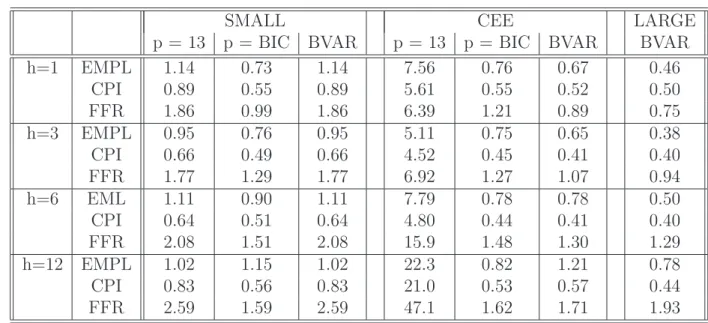
Table 2 presents the results forSMALL andCEE. We report results forp= 13 lags and for the number of lags p selected by the BIC criterion. For comparison, we also recall from Table 1 the results for the Bayesian estimation of the model of the same size. We do not report estimates for p= 13 and BIC selection for the large model since for that size the estimation by OLS and p = 13 is unfeasible. However, we recall in the last column the results for the large model estimated by Bayesian approach.
These results show that for the model SMALL, BIC selection results in the best forecast accuracy. For the larger CEE model, the classical VAR with lags selected by BIC and the BVAR perform similarly. Both specifications are, however, outperformed by the large Bayesian VAR.
3.2
The Bayesian VAR and the Factor Augmented VAR (FAVAR)
Factor models have been shown to be successful at forecasting macroeconomic variables with a large number of predictors. It is therefore natural to compare forecasting results based on the Bayesian VAR with those produced by factor models where factors are
3However, due to their timeliness, conjunctural information, may be important for improving early
estimates of variables in the current quarter as argued by Giannone, Reichlin, and Small (2008). This is an issue which we do not explore here.
Table 2: Relative MSFE, OLS and BVAR
SMALL CEE LARGE
p = 13 p = BIC BVAR p = 13 p = BIC BVAR BVAR
h=1 EMPL 1.14 0.73 1.14 7.56 0.76 0.67 0.46 CPI 0.89 0.55 0.89 5.61 0.55 0.52 0.50 FFR 1.86 0.99 1.86 6.39 1.21 0.89 0.75 h=3 EMPL 0.95 0.76 0.95 5.11 0.75 0.65 0.38 CPI 0.66 0.49 0.66 4.52 0.45 0.41 0.40 FFR 1.77 1.29 1.77 6.92 1.27 1.07 0.94 h=6 EML 1.11 0.90 1.11 7.79 0.78 0.78 0.50 CPI 0.64 0.51 0.64 4.80 0.44 0.41 0.40 FFR 2.08 1.51 2.08 15.9 1.48 1.30 1.29 h=12 EMPL 1.02 1.15 1.02 22.3 0.82 1.21 0.78 CPI 0.83 0.56 0.83 21.0 0.53 0.57 0.44 FFR 2.59 1.59 2.59 47.1 1.62 1.71 1.93
Notes: Table reports MSFE relative to that from the benchmark model (random walk with drift) for employment (EMPL), CPI and federal funds rate (FFR) for different forecast horizons h and different models. SMALL, CEE refer to the VARs with 3 and 7 variables, respectively. Those systems are estimated by OLS with number of lags fixed to 13 or chosen by the BIC. The evaluation period is 1971-2003. For comparison the results of Bayesian estimation of the two models and of the large model are also provided.
estimated by principal components.
A comparison of forecasts based, alternatively, on Bayesian regression and principal components regression has recently been performed by De Mol, Giannone, and Reichlin (2008) and Giacomini and White (2006). In those exercises, variables are transformed to stationarity as is standard practice in the principal components literature. Moreover, the Bayesian regression is estimated as a single equation.
Here we want to perform an exercise in which factor models are compared with the standard VAR specification in the macroeconomic literature where variables are treated in levels and the model is estimated as a system rather than as a set of single equations. Therefore, for comparison with the VAR, rather than considering principal components regression, we will use a small VAR (with variables in levels) augmented by principal components extracted from the panel (in differences). This is the FAVAR method ad-vocated by Bernanke, Boivin, and Eliasz (2005) and discussed by Stock and Watson (2005b).
More precisely, principal components are extracted from the large panel of 131 vari-ables. Variables are first made stationary by taking first differences wherever we have
imposed a random walk priorδi = 1. Then, as principal components are not scale invari-ant, variables are standardised and the factors are computed on standardised variables, recursively at each point T in the evaluation sample.
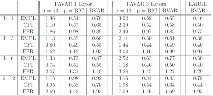
We consider specifications with one and three factors and look at different lag selection for the VAR. We set p = 13, as in Bernanke, Boivin, and Eliasz (2005) and we also consider thepselected by the BIC criterion. Moreover, we consider Bayesian estimation of the FAVAR (BFAVAR), taking p= 13 and choosing the shrinkage hyperparameter λ that results in the same in-sample fit as in the exercise summarized in Table 1.
Results are reported in Table 3 (the last column recalls results from the large Bayesian VAR for comparison).
Table 3: Relative MSFE, FAVAR
FAVAR 1 factor FAVAR 3 factors LARGE p = 13 p = BIC BVAR p = 13 p = BIC BVAR BVAR
h=1 EMPL 1.36 0.54 0.70 3.02 0.52 0.65 0.46 CPI 1.10 0.57 0.65 2.39 0.52 0.58 0.50 FFR 1.86 0.98 0.89 2.40 0.97 0.85 0.75 h=3 EMPL 1.13 0.55 0.68 2.11 0.50 0.61 0.38 CPI 0.80 0.49 0.55 1.44 0.44 0.49 0.40 FFR 1.62 1.12 1.03 3.08 1.16 0.99 0.94 h=6 EMPL 1.33 0.73 0.87 2.52 0.63 0.77 0.50 CPI 0.74 0.52 0.55 1.18 0.46 0.50 0.40 FFR 2.07 1.31 1.40 3.28 1.45 1.27 1.29 h=12 EMPL 1.15 0.98 0.92 3.16 0.84 0.83 0.78 CPI 0.95 0.58 0.70 1.98 0.54 0.64 0.44 FFR 2.69 1.43 1.93 7.09 1.46 1.69 1.93
Notes: Table reports MSFE for the FAVAR model relative to that from the benchmark model (random walk with drift) for employment (EMPL), CPI and federal funds rate (FFR) for different forecast horizons h. FAVAR includes 1 or 3 factors and the three variables of interest. The system is estimated by OLS with number of lags fixed to 13 or chosen by the BIC and by applying Bayesian shrinkage. The evaluation period is 1971-2003. For comparison the results from large Bayesian VAR are also provided.
The Table shows that the FAVAR is in general outperformed by the BVAR of large size and that therefore Bayesian VAR is a valid alternative to factor based forecasts, at least to those based on the FAVAR method.4 We should also note that BIC lag selection generates the best results for the FAVAR while the original specification of Bernanke, Boivin, and Eliasz (2005) withp= 13 performs very poorly due to its lack of parsimony.
4De Mol, Giannone, and Reichlin (2008) show that for regressions based on stationary variables,
3.3
Prior on the sum of coefficients
The literature has suggested that improvement in forecasting performance can be ob-tained by imposing additional priors that constrain the sum of coefficients (see e.g. Sims, 1992; Sims and Zha, 1998; Robertson and Tallman, 1999). This is the same as imposing “inexact differencing” and it is a simple modification of the Minnesota prior involving linear combinations of the VAR coefficients, cf. Doan, Litterman, and Sims (1984). Let us rewrite the VAR of equation (1) in its error correction form:
ΔYt=c−(In−A1− · · · −Ap)Yt−1+B1ΔYt−1+· · ·+Bp−1ΔYt−p+1+ut. (8)
A VAR in first differences implies the restriction (In−A1− · · · −Ap) = 0. We follow
Doan, Litterman, and Sims (1984) and set a prior that shrinks Π = (In−A1− · · · −Ap)
to zero. This can be understood as “inexact differencing” and in the literature it is usually implemented by adding the following dummy observations (cf. Section 2):
Yd= diag(δ1μ1, . . . , δnμn)/τ Xd=
(1 2 . . . p)⊗diag(δ1μ1, . . . , δnμn)/τ 0n×1
. (9) The hyperparameterτ controls for the degree of shrinkage: asτ goes to zero we approach the case of exact differences and, as τ goes to∞, we approach the case of no shrinkage. The parameter μi aims at capturing the average level of variable yit. Although the parameters should in principle be set using only prior knowledge, we follow common practice5 and set the parameter equal to the sample average of yit. Our approach is to
set a loose prior with τ = 10λ. The overall shrinkageλ is again selected so as to match the fit of the small specification estimated by OLS.
Table 4 reports results from the forecast evaluation of the specification with the sum of coefficient prior. They show that, qualitatively, results do not change for the smaller models, but improve significantly for the MEDIUM and LARGE specifications. In par-ticular, the poor results for the federal funds rate discussed in Table 1 are now improved. Both the MEDIUM and LARGE models outperform the random walk forecasts at all the horizons considered. Overall, the sum of coefficient prior improves forecast accuracy, confirming the findings of Robertson and Tallman (1999).
Table 4: Relative MSFE, BVAR with the prior on the sum of coefficients SMALL CEE MEDIUM LARGE
EMPL 1.14 0.68 0.53 0.44 h=1 CPI 0.89 0.57 0.49 0.49 FFR 1.86 0.97 0.75 0.74 EMPL 0.95 0.60 0.49 0.36 h=3 CPI 0.66 0.44 0.39 0.37 FFR 1.77 1.28 0.85 0.82 EMPL 1.11 0.65 0.58 0.44 h=6 CPI 0.64 0.45 0.37 0.36 FFR 2.08 1.40 0.96 0.92 EMPL 1.02 0.65 0.60 0.50 h=12 CPI 0.83 0.55 0.43 0.40 FFR 2.59 1.61 0.93 0.92
Notes for Table 1 apply. The difference is that the prior on the sum of coefficients has been added. The tightness of this prior is controlled by the hyperparameter τ = 10λ, whereλ controls the overall tightness.
4
Structural analysis:
impulse response functions
and variance decomposition
We now turn to the structural analysis and estimate, on the basis of BVARs of different size, the impulse responses of different variables to a monetary policy shock.
To this purpose, we identify the money shock by using a recursive identification scheme adapted to a large number of variables. We follow Bernanke, Boivin, and Eliasz (2005), Christiano, Eichenbaum, and Evans (1999) and Stock and Watson (2005b) and divide the variables in the panel into two categories: slow- and fast-moving. Roughly speaking the former group contains real variables and prices while the latter consists of finan-cial variables (the precise classification is given in the Appendix A). The identifying assumption is that slow-moving variables do not respond contemporaneously to a mon-etary policy shock and that the information set of the monmon-etary authority contains only past values of the fast-moving variables.
The monetary policy shock is identified as follows. We order the variables as Yt = (Xt, rt, Zt), whereXt contains then1 slowly moving variables, rt is the monetary policy
instrument and Zt contains the n2 fast moving variables and we assume that the mone-tary policy shock is orthogonal to all other shocks driving the economy. LetB =CD1/2 be the n×n lower diagonal Cholesky matrix of the covariance of the residuals of the
reduced form VAR, that isCDC =E[utut] = Ψ and D= diag(Ψ).
Let et be the following linear transformation of the VAR residuals: et = (e1t, ..., ent) =
C−1u
t. The monetary policy shock is the row of et corresponding to the position of rt,
that is en1+1,t.
The Structural VAR can hence be written as
A0Yt =ν+A1Yt−1+...+ApYt−p+et, et∼W N(0, D),
where ν=C−1c, A
0 =C−1 and Aj =C−1Aj, j = 1, ..., p.
Our experiment consists in increasing contemporaneously the federal funds rate by one hundred basis points.
Since we have just identification, the impulse response functions are easily computed following Canova (1991) and Gordon and Leeper (1994) by generating draws from the posterior of (A1, ..., Ap,Ψ). For each draw Ψ we compute B and C and we can then
calculate Aj, j = 0, ..., p.
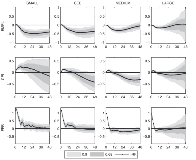
We report the results for the same overall shrinkage as given in Table 4. Estimation is based on the sample 1961-2002. The number of lags remains 13. Results are reported for the specification including sum of coefficients priors since it is the one providing the best forecast accuracy and also because, for the LARGE model, without sum of coefficients prior, the posterior coverage intervals of the impulse response functions become very wide for horizons beyond two years, eventually becoming explosive (cf. the Appendix, Figure C.1). For the other specifications, the additional prior does not change the results. Figure 1 displays the impulse response functions for the four models under consideration and for the three key variables. The shaded regions indicate the posterior coverage intervals corresponding to 90 and 68 percent confidence levels. Table 5 reports the percentage share of the monetary policy shock in the forecast error variance for chosen forecast horizons.
Results show that, as we add information, impulse response functions slightly change in shape which suggests that conditioning on realistic informational assumptions is impor-tant for structural analysis as well as for forecasting. In particular, it is confirmed that adding variables helps in resolving the price puzzle (on this point see also Bernanke and Boivin, 2003; Christiano, Eichenbaum, and Evans, 1999). Moreover, for larger mod-els the effect of monetary policy on employment becomes less persistent, reaching a peak at about one year horizon. For the large model, the non-systematic component
of monetary policy becomes very small, confirming results in Giannone, Reichlin, and Sala (2004) obtained on the basis of a factor model. It is also important to stress that impulse responses maintain the expected sign for all specifications.
Figure 1: Impulse response functions, BVAR with the prior on the sum of coefficients
0 12 24 36 48 −1 −0.5 0 EMPL SMALL 0 12 24 36 48 −1.5 −1 −0.5 0 CPI 0 12 24 36 48 −0.5 0 0.5 1 FFR 0 12 24 36 48 −1 −0.5 0 CEE 0 12 24 36 48 −1.5 −1 −0.5 0 0 12 24 36 48 −0.5 0 0.5 1 0 12 24 36 48 −1 −0.5 0 MEDIUM 0 12 24 36 48 −1.5 −1 −0.5 0 0 12 24 36 48 −0.5 0 0.5 1 0 12 24 36 48 −1 −0.5 0 LARGE 0 12 24 36 48 −1.5 −1 −0.5 0 0 12 24 36 48 −0.5 0 0.5 1 0.9 0.68 IRF
Notes: Figure presents the impulse response functions to a monetary policy shock and the corresponding posterior coverage intervals at 0.68 and 0.9 level for employment (EMPL), CPI and federal funds rate (FFR). SMALL, CEE, MEDIUM and LARGE refer to the VARs with 3, 7, 20 and 131 variables, respectively. The prior on the sum of coefficients has been added with the hyperparameter τ= 10λ.
The same features can be seen from the variance decomposition, reported in Table 5. As the size of the model increases, the size of the monetary shock decreases. This is not surprising, given the fact that the forecast accuracy improves with size, but it highlights an important point. If realistic informational assumptions are not taken into consideration, we may mix structural shocks with miss-specification errors. Clearly, the assessment of the importance of the systematic component of monetary policy depends
Table 5: Variance decomposition, BVAR with the prior on the sum of coefficients Hor SMALL CEE MEDIUM LARGE
EMPL 1 0 0 0 0 3 0 0 0 0 6 1 1 2 2 12 5 7 7 5 24 12 14 13 8 36 18 19 14 7 48 23 23 12 6 CPI 1 0 0 0 0 3 3 2 1 2 6 7 5 3 3 12 6 3 1 1 24 2 1 1 1 36 1 2 3 2 48 1 3 5 3 FFR 1 99 97 93 51 3 90 84 71 33 6 74 66 49 21 12 46 39 30 14 24 26 21 18 9 36 21 17 16 7 48 18 15 16 7
Notes: Table reports the percentage share of the monetary policy shock in the forecast error variance for chosen forecast horizons for employment (EMPL), CPI and federal funds rate (FFR). SMALL, CEE, MEDIUM and LARGE refer to the VARs with 3, 7, 20 and 131 variables, respectively. The prior on the sum of coefficients has been added with the hyperparameterτ= 10λ. The models have been estimated in the sample 1961-2002.
on the conditioning information set used by the econometrician and this may differ from that which is relevant for policy decisions. Once the realistic feature of large information is taken into account by the econometrician, the estimate of the size of the non-systematic component decreases.
Let us now comment on the impulse response functions of the monetary policy shock on all the twenty variables considered in the MEDIUM model. Impulse responses and variance decomposition for all the variables and models are reported in the Appendix, Tables C.1-C.4.
Figure 2 reports the impulses for both the MEDIUM and LARGEmodel as well as the posterior coverage intervals produced by the LARGE model.
Figure 2: Impulse response functions for model MEDIUM and LARGE, BVAR with the prior on the sum of coefficients
0 12 24 36 48 −1 −0.5 0 0.5 EMPL 0 12 24 36 48 −2 −1 0 1 CPI 0 12 24 36 48 −4 −3 −2 −1 0 COMM PR 0 12 24 36 48 −0.5 0 0.5 INCOME 0 12 24 36 48 −0.5 0 0.5 1 CONSUM 0 12 24 36 48 −2 −1 0 1 IP 0 12 24 36 48 −1 −0.5 0 0.5 1 CAP UTIL 0 12 24 36 48 −0.5 0 0.5 UNEMPL 0 12 24 36 48 −5 0 5 HOUS START 0 12 24 36 48 −2 −1 0 1 PPI 0 12 24 36 48 −1 −0.5 0 0.5 PCE DEFL 0 12 24 36 48 −1 −0.5 0 0.5 HOUR EARN 0 12 24 36 48 −1 0 1 2 FFR 0 12 24 36 48 −1 −0.5 0 0.5 1 M1 0 12 24 36 48 −0.5 0 0.5 1 M2 0 12 24 36 48 −2 −1 0 1 2 TOT RES 0 12 24 36 48 −2 −1 0 1 2 NBORR RES 0 12 24 36 48 −4 −2 0 2 S&P 0 12 24 36 48 −0.5 0 0.5 TB YIELD 0 12 24 36 48 −1 0 1 2 EXR
0.9 0.68 IRF Large IRF Medium
Notes: Figure presents the impulse response functions to a monetary policy shock from MEDIUM and LARGE specifications for all the variables included in MEDIUM. The posterior coverage intervals at 0.68 and 0.9 level correspond to the LARGE specification. The prior on the sum of coefficients has been added with the hyperparameterτ= 10λ.
Let us first remark that the impulse responses are very similar for the two specifications and in most cases those produced by theMEDIUMmodel are within the coverage inter-vals of theLARGE model. This reinforces our conjecture that a VAR with 20 variables is sufficient to capture the relevant shocks and the extra information is redundant. Responses have the expected sign. First of all, a monetary contraction has a negative effect on real economic activity. Beside employment, consumption, industrial production and capacity utilization respond negatively for two years and beyond. By contrast, the effect on all nominal variables is negative. Since the model contains more than the standard nominal and real variables, we can also study the effect of monetary shocks on housing starts, stock prices and exchange rate. The impact on housing starts is very large and negative and it lasts about one year. The effect on stock prices is significantly negative for about one year. Lastly, the exchange rate appreciation is persistent in both nominal and real terms as found in Eichenbaum and Evans (1995).
5
Summary
This paper assesses the performance of Bayesian VAR for monetary models of different size. We consider standard specifications in the literature with three and seven macroe-conomic variables and also study a VARs with twenty and a hundred and thirty variables. The latter considers sectoral and conjunctural information in addition to macroeconomic information. We examine both forecasting accuracy and structural analysis of the effect of a monetary policy shock.
The setting of the prior follows standard recommendations in the Bayesian literature ex-cept for the fact that the overall tightness hyperparameter is set in relation to the model size. As the model becomes larger, we increase the overall shrinkage so as to maintain the same in-sample fit across models and guarantee a meaningful model comparison. Overall, results show that a standard Bayesian VAR model is an appropriate tool for large panels of data. Not only a Bayesian VAR estimated over one hundred variables is feasible, but it produces better forecasting results than the typical seven variables VAR considered in the literature. The structural analysis on the effect of the monetary shock shows that a VAR based on twenty variables produces results that remain robust when the model is enlarged further.
References
Bernanke, B., J. Boivin, and P. Eliasz (2005): “Measuring Monetary Policy: A
Factor Augmented Autoregressive (FAVAR) Approach,” Quarterly Journal of
Eco-nomics, 120, 387–422.
Bernanke, B. S., and J. Boivin (2003): “Monetary policy in a data-rich
environ-ment,” Journal of Monetary Economics, 50(3), 525–546.
Boivin, J., and S. Ng (2005): “Understanding and Comparing Factor-Based
Fore-casts,”International Journal of Central Banking, 3, 117–151.
Canova, F. (1991): “The Sources of Financial Crisis: Pre- and Post-Fed Evidence,”
International Economic Review, 32(3), 689–713.
Canova, F., and M. Ciccarelli (2004): “Forecasting and turning point predictions
in a Bayesian panel VAR model,”Journal of Econometrics, 120(2), 327–359.
Christiano, L. J., M. Eichenbaum, and C. Evans (1996): “The Effects of
Mon-etary Policy Shocks: Evidence from the Flow of Funds,” The Review of Economics
and Statistics, 78(1), 16–34.
Christiano, L. J., M. Eichenbaum, and C. L. Evans (1999): “Monetary policy
shocks: What have we learned and to what end?,” in Handbook of Macroeconomics, ed. by J. B. Taylor,and M. Woodford, vol. 1, chap. 2, pp. 65–148. Elsevier.
D’Agostino, A., andD. Giannone(2006): “Comparing alternative predictors based
on large-panel factor models,” Working Paper Series 680, European Central Bank.
De Mol, C., D. Giannone, and L. Reichlin (2008): “Forecasting using a large
number of predictors - Is Bayesian regression a valid alternative to principal compo-nents?,”Journal of Econometrics, forthcoming.
di Mauro, F., L. V. Smith, S. Dees, and M. H. Pesaran (2007): “Exploring the
international linkages of the euro area: a global VAR analysis,” Journal of Applied
Econometrics, 22(1), 1–38.
Doan, T., R. Litterman, and C. A. Sims (1984): “Forecasting and Conditional
Eichenbaum, m., and C. L. Evans (1995): “Some Empirical Evidence on the
Ef-fects of Shocks to Monetary Policy on Exchange Rates,” The Quarterly Journal of
Economics, 110(4), 975–1009.
Forni, M., D. Giannone, M. Lippi, and L. Reichlin (2008): “Opening the Black
Box: Structural Factor Models versus Structural VARs,” Econometric Theory, forth-coming.
Forni, M., M. Hallin, M. Lippi, and L. Reichlin (2000): “The Generalized
Dy-namic Factor Model: identification and estimation,”Review of Economics and Statis-tics, 82, 540–554.
(2003): “Do Financial Variables Help Forecasting Inflation and Real Activity in the Euro Area?,” Journal of Monetary Economics, 50, 1243–55.
(2005): “The Generalized Dynamic Factor Model: one-sided estimation and forecasting,” Journal of the American Statistical Association, 100, 830–840.
Giacomini, R., and H. White (2006): “Tests of Conditional Predictive Ability,”
Econometrica, 74(6), 1545–78.
Giannone, D., andL. Reichlin(2006): “Does information help recovering structural
shocks from past observations?,”Journal of the European Economic Association, 4(2-3), 455–465.
Giannone, D., L. Reichlin, and L. Sala(2004): “Monetary Policy in Real Time,”
in NBER Macroeconomics Annual, ed. by M. Gertler, and K. Rogoff, pp. 161–200.
MIT Press.
Giannone, D., L. Reichlin, and D. Small (2008): “Nowcasting: The real-time
in-formational content of macroeconomic data,”Journal of Monetary Economics, 55(4), 665–676.
Gordon, D. B., and E. M. Leeper (1994): “The Dynamic Impacts of Monetary
Policy: An Exercise in Tentative Identification,”Journal of Political Economy, 102(6), 1228–47.
Hamilton, J. D. (2006): “Computing power and the power of econometrics,”
Manuscript, University of California, San Diego.
Kadiyala, K. R., and S. Karlsson(1997): “Numerical Methods for Estimation and
Kim, S. (2001): “International transmission of U.S. monetary policy shocks: Evidence
from VAR’s,” Journal of Monetary Economics, 48(2), 339–372.
Leeper, E. M., C. Sims, and T. Zha (1996): “What Does Monetary Policy Do?,”
Brookings Papaers on Economic Activity, 1996(2), 1–78.
Litterman, R. (1986a): “Forecasting With Bayesian Vector Autoregressions – Five
Years of Experience,” Journal of Business and Economic Statistics, 4, 25–38.
(1986b): “A statistical approach to economic forecasting,”Journal of Business
and Economic Statistics, 4(1), 1–4.
Mackowiak, B. (2006): “What does the Bank of Japan do to East Asia?,”Journal of
International Economics, 70(1), 253–270.
(2007): “External shocks, U.S. monetary policy and macroeconomic fluctua-tions in emerging markets,” Journal of Monetary Economics, 54(8), 2512–2520.
Marcellino, M., J. H. Stock, and M. W. Watson (2003): “Macroeconomic
forecasting in the euro area: Country specific versus area-wide information,” European
Economic Review, 47(1), 1–18.
Robertson, J. C., and E. W. Tallman(1999): “Vector autoregressions: forecasting
and reality,” Economic Review, (Q1), 4–18.
Sims, C. A. (1992): “Bayesian Inference for Multivariate Time Series with Trend,”
Mimeo.
Sims, C. A., and T. Zha (1998): “Bayesian Methods for Dynamic Multivariate
Mod-els,” International Economic Review, 39(4), 949–68.
Stock, J. H., andM. W. Watson(2002a): “Forecasting Using Principal Components
from a Large Number of Predictors,”Journal of the American Statistical Association, 97, 147–162.
(2002b): “Macroeconomic Forecasting Using Diffusion Indexes.,” Journal of
Business and Economics Statistics, 20, 147–162.
(2005a): “An Empirical Comparison Of Methods For Forecasting Using Many Predictors,” Manuscript, Princeton University.
(2005b): “Implications of Dynamic Factor Models for VAR Analysis,” Unpub-lished manuscript, Princeton University.
Uhlig, H. (2004): “What moves GNP?,” Econometric Society 2004 North American
Description
of
the
data
set
Series Slo w/F ast SMALL CEE MEDIUM Log R W prior EMPLO YEES ON NONF ARM P A YR OLLS -TOT AL PRIV A TE S X X X X X CPI-U: ALL ITEMS (82-84=100,SA) S X X X X X INDEX OF SENSITIVE MA TERIALS PRICES (1990=100)(BCI-99A) S X X X X PERSONAL INCOME LESS TRANSFER P A YMENTS (AR, BIL. CHAIN 2000 $) S X X X R REAL CONSUMPTION (A C) A0M224/GMDC S X X X INDUSTRIAL PR ODUCTION INDEX -TOT AL INDEX S X X X CAP A CITY UITLIZA TION (MF G) S X X UNEMPLO YMENT RA TE: ALL W ORKERS, 16 YEARS & O VER (%,SA) S X X HOUSING ST AR TS:NONF ARM(1947-58);TOT AL F ARM&NONF ARM(1959-)(THOUS.,SA) S X X PR ODUCER PRICE INDEX: FINISHED GOODS (1982=100,SA) S X X X PCE,IMPL PR DEFL:PCE (1987=100) S X X X A V G HRL Y EARNINGS OF PR OD OR NONSUP W ORKERS ON PRIV NONF ARM P A YR OLLS -GOODS PR ODUCING S X X X PERSONAL INCOME (AR, BIL. CHAIN 2000 $) S X X MANUF A CTURING AND TRADE SALES (MIL. CHAIN 1996 $) S X X SALES OF RET AIL STORES (MIL. CHAIN 2000 $) S X X INDUSTRIAL PR ODUCTION INDEX -PR ODUCTS, TOT AL S X X INDUSTRIAL PR ODUCTION INDEX -FINAL PR ODUCTS S X X INDUSTRIAL PR ODUCTION INDEX -CONSUMER GOODS S X X INDUSTRIAL PR ODUCTION INDEX -DURABLE CONSUMER GOODS S X X INDUSTRIAL PR ODUCTION INDEX -NONDURABLE CONSUMER GOODS S X X INDUSTRIAL PR ODUCTION INDEX -BUSINESS EQUIPMENT S X X INDUSTRIAL PR ODUCTION INDEX -MA TERIALS S X X INDUSTRIAL PR ODUCTION INDEX -DURABLE GOODS MA TERIALS S X X INDUSTRIAL PR ODUCTION INDEX -NONDURABLE GOODS MA TERIALS S X X INDUSTRIAL PR ODUCTION INDEX -MANUF A CTURING (SIC) S X X INDUSTRIAL PR ODUCTION INDEX -RESIDENTIAL UTILITIES S X X INDUSTRIAL PR ODUCTION INDEX -FUELS S X X NAPM PR ODUCTION INDEX (PER CENT) S INDEX OF HELP-W ANTED AD VER TISING IN NEWSP APERS (1967=100;SA) S X EMPLO YMENT: RA TIO; HELP-W ANTED ADS:NO. UNEMPLO YED CLF S X CIVILIAN LABOR F OR CE: EMPLO YED, TOT AL (THOUS.,SA) S X X G CIVILIAN LABOR F OR CE: EMPLO YED, NONA GRIC.INDUSTRIES (THOUS.,SA) S X X UNEMPLO Y.BY DURA TION: A VERA GE(MEAN)DURA TION IN WEEKS (SA) S X UNEMPLO Y.BY DURA TION: PERSONS UNEMPL.LESS THAN 5 WKS (THOUS.,SA) S X X UNEMPLO Y.BY DURA TION: PERSONS UNEMPL.5 TO 14 WKS (THOUS.,SA) S X X UNEMPLO Y.BY DURA TION: PERSONS UNEMPL.15 WKS + (THOUS.,SA) S X X UNEMPLO Y.BY DURA TION: PERSONS UNEMPL.15 TO 26 WKS (THOUS.,SA) S X X UNEMPLO Y.BY DURA TION: PERSONS UNEMPL.27 WKS + (THOUS.,SA) S X X A VERA GE WEEKL Y INITIAL CLAIMS, UNEMPLO Y. INSURANCE (THOUS.) S X X EMPLO YEES ON NONF ARM P A YR OLLS -GOODS-PR ODUCING S X X EMPLO YEES ON NONF ARM P A YR OLLS -MINING S X X EMPLO YEES ON NONF ARM P A YR OLLS -CONSTR UCTION S X X EMPLO YEES ON NONF ARM P A YR OLLS -MANUF A CTURING S X X EMPLO YEES ON NONF ARM P A YR OLLS -DURABLE GOODS S X X EMPLO YEES ON NONF ARM P A YR OLLS -NONDURABLE GOODS S X X EMPLO YEES ON NONF ARM P A YR OLLS -SER VICE-PR O VIDING S X X EMPLO YEES ON NONF ARM P A YR OLLS -TRADE, TRANSPO RTAT ION, AND UTILITIES S X X EMPLO YEES ON NONF ARM P A YR OLLS -WHOLESALE TRADE S X X EMPLO YEES ON NONF ARM P A YR OLLS -RET AIL TRADE S X X EMPLO YEES ON NONF ARM P A YR OLLS -FINANCIAL A CTIVITIES S X X EMPLO YEES ON NONF ARM P A YR OLLS -GO VERNMENT S X X EMPLO YEE HOURS IN NONA G. EST ABLISHMENTS (AR, BIL. HOURS) S X X A V G WEEKL Y HRS OF PR OD OR NONSUP W ORKERS ON PRIV NONF AR P A YR OLLS -GOODS PR ODUCING S A V G WEEKL Y HRS OF PR OD OR NONSUP W ORKERS ON PRIV NONF AR P A YR OLLS -MF G O VETIME HRS S X A VERA GE WEEKL Y HOURS, MF G. (HOURS) S NAPM EMPLO YMENT INDEX (PER CENT) S HOUSING ST AR TS:NOR THEAST (THOUS.U.,S.A.) S X HOUSING ST AR TS:MID WEST(THOUS.U.,S.A.) S X HOUSING ST AR TS:SOUTH (THOUS.U.,S.A.) S X HOUSING ST AR TS:WEST (THOUS.U.,S.A.) S X HOUSING A UTHORIZED: TOT AL NEW PRIV HOUSING UNITS (THOUS.,SAAR) S X HOUSES A UTHORIZED BY BUILD. PERMITS:NOR THEAST(THOUS.U.,S.A.) S X HOUSES A UTHORIZED BY BUILD. PERMITS:MID WEST(THOUS.U.,S.A.) S X HOUSES A UTHORIZED BY BUILD. PERMITS:SOUTH(THOUS.U.,S.A.) S XHOUSES A UTHORIZED BY BUILD. PERMITS:WEST(THOUS.U.,S.A.) S X PUR CHASING MANA GERS’ INDEX (SA) S NAPM NEW ORDERS INDEX (PER CENT) S NAPM VENDOR DELIVERIES INDEX (PER CENT) S NAPM INVENTORIES INDEX (PER CENT) S MFRS’ NEW ORDERS, CONSUMER GOODS AND MA TERIALS (BIL. CHAIN 1982 $) S X X MFRS’ NEW ORDERS, DURABLE GOODS INDUSTRIES (BIL. CHAIN 2000 $) S X X MFRS’ NEW ORDERS, NONDEFENCE CAPIT AL GOODS (MIL. CHAIN 1982 $) S X X MFRS’ UNFILLED ORDERS, DURABLE GOODS INDUS. (BIL. CHAIN 2000 $) S X X MANUF A CTURING AND TRADE INVENTORIES (BIL. CHAIN 2000 $) S X X RA TIO, MF G. AND TRADE INVENTORIES TO SALES BASED ON CHAIN 2000 $) S X PR ODUCER PRICE INDEX:FINISHED CONSUMER GOODS (1982=100,SA) S X X PR ODUCER PRICE INDEX:INTERMED MA T.SUPPLIES & COMPONENTS(1982=100,SA) S X X PR ODUCER PRICE INDEX:CR UDE MA TERIALS (1982=100,SA) S X X NAPM COMMODITY PRICES INDEX (PER CENT) S CPI-U: APP AREL & UPKEEP (1982-84=100,SA) S X X CPI-U: TRANSPOR T A TION (1982-84=100,SA) S X X CPI-U: MEDICAL CARE (1982-84=100,SA) S X X CPI-U: COMMODITIES (1982-84=100,SA) S X X CPI-U: DURABLES (1982-84=100,SA) S X X CPI-U: SER VICES (1982-84=100,SA) S X X CPI-U: ALL ITEMS LESS F OOD (1982-84=100,SA) S X X CPI-U: ALL ITEMS LESS SHEL TER (1982-84=100,SA) S X X CPI-U: ALL ITEMS LESS MIDICAL CARE (1982-84=100,SA) S X X PCE,IMPL PR DEFL:PCE; DURABLES (1987=100) S X X PCE,IMPL PR DEFL:PCE; NONDURABLES (1996=100) S X X PCE,IMPL PR DEFL:PCE; SER VICES (1987=100) S X X A V G HRL Y EARNINGS OF PR OD OR NONSUP W ORKERS ON PRIV NONF ARM P A YR OLLS -CONSTR UCTION S X X A V G HRL Y EARNINGS OF PR OD OR NONSUP W ORKERS ON PRIV NONF ARM P A YR OLLS -MANUF A CTURING S X X U. OF MICH. INDEX OF CONSUMER EXPECT A TIONS(BCD-83) S X INTEREST RA TE: FEDERAL FUNDS (EFFECTIVE) (% PER ANNUM,NSA) R X X X X MONEY STOCK:M2(M1+O’NITE RPS,EUR O$,G/P&B/D MMMFS&SA V&SM TIME DEP(BIL.$,SA) F X X X X DEPOSITOR Y INST RESER VES:TOT AL,ADJ F OR RESER VE REQ CHGS(MIL.$,SA) F X X X X DEPOSITOR Y INST RESER VES:NONBORR O WED,ADJ RES REQ CHGS(MIL.$,SA) F X X X X MONEY STOCK: M1(CURR,TRA V.CKS,DEM DEP ,OTHER CK’ABLE DEP)(BIL.$,SA) F X X X S&P’S COMMON STOCK PRICE INDEX: COMPOSITE (1941-43=10) F X X X INTEREST RA TE: U.S.TREASUR Y CONST MA TURITIES,10-YR.(% PER ANN,NSA) F X X UNITED ST A TES;EFFECTIVE EX CHANGE RA TE(MERM)(INDEX NO.) F X X X MONEY STOCK: M3(M2+LG TIME DEP ,TERM RP’S&INST ONL Y MMMFS)(BIL.$,SA) F X X MONEY SUPPL Y -M2 IN 1996 DOLLARS (BCI) F X X MONET AR Y BASE, ADJ F OR RESER VE REQUIREMENT CHANGES(MIL.$,SA) F X X COMMER CIAL & INDUSTRIAL LO ANS OUST ANDING IN 1996 DOLLARS (BCI) F X X WKL Y RP LG COM’L BANKS:NET CHANGE COM’L & INDUS LO ANS(BIL.$,SAAR) F V CONSUMER CREDIT OUTST ANDING -NONREV OL VING(G19) F X X RA TIO, CONSUMER INST ALLMENT CREDIT TO PERSONAL INCOME (PER CENT) F X S&P’S COMMON STOCK PRICE INDEX: INDUSTRIALS (1941-43=10) F X X S&P’S COMPOSITE COMMON STOCK: DIVIDEND YIELD (% PER ANNUM) F X S&P’S COMPOSITE COMMON STOCK: PRICE-EARNINGS RA TIO (%,NSA) F X X COMMER CIAL P APER RA TE (A C) F X INTEREST RA TE: U.S.TREASUR Y BILLS,SEC MKT,6-MO.(% PER ANN,NSA) F X INTEREST RA TE: U.S.TREASUR Y CONST MA TURITIES,1-YR.(% PER ANN,NSA) F X INTEREST RA TE: U.S.TREASUR Y CONST MA TURITIES,5-YR.(% PER ANN,NSA) F X INTEREST RA TE: U.S.TREASUR Y BILLS,SEC MKT,3-MO.(% PER ANN,NSA) F X C BOND YIELD: MOOD Y’S AAA CORPORA TE (% PER ANNUM) F X C BOND YIELD: MOOD Y’S BAA CORPORA TE (% PER ANNUM) F X CP90-FYFF F FYGM3-FYFF F FYGM6-FYFF F FYGT1-FYFF F FYGT5-FYFF F FYGT10-FYFF F C FY AAA C-FYFF F C FYBAA C-FYFF F F OREIGN EX CHANGE RA TE: SWITZERLAND (SWISS FRANC PER U.S.$) F X X F OREIGN EX CHANGE RA TE: JAP AN (YEN PER U.S.$) F X X F OREIGN EX CHANGE RA TE: UNITED KINGDOM (CENTS PER POUND) F X X F OREIGN EX CHANGE RA TE: CANAD A (CANADIAN $ PER U.S.$) F X X
B
Relative MSFE for different in-sample fits
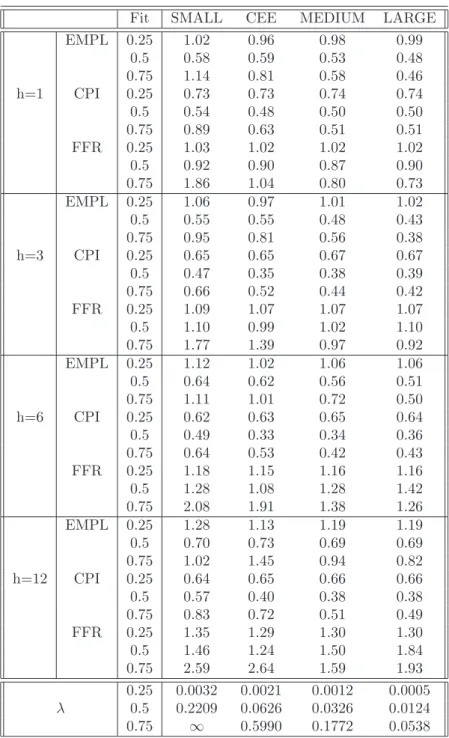
Table B.1: Relative MSFE, BVARFit SMALL CEE MEDIUM LARGE
EMPL 0.25 1.02 0.96 0.98 0.99 0.5 0.58 0.59 0.53 0.48 0.75 1.14 0.81 0.58 0.46 h=1 CPI 0.25 0.73 0.73 0.74 0.74 0.5 0.54 0.48 0.50 0.50 0.75 0.89 0.63 0.51 0.51 FFR 0.25 1.03 1.02 1.02 1.02 0.5 0.92 0.90 0.87 0.90 0.75 1.86 1.04 0.80 0.73 EMPL 0.25 1.06 0.97 1.01 1.02 0.5 0.55 0.55 0.48 0.43 0.75 0.95 0.81 0.56 0.38 h=3 CPI 0.25 0.65 0.65 0.67 0.67 0.5 0.47 0.35 0.38 0.39 0.75 0.66 0.52 0.44 0.42 FFR 0.25 1.09 1.07 1.07 1.07 0.5 1.10 0.99 1.02 1.10 0.75 1.77 1.39 0.97 0.92 EMPL 0.25 1.12 1.02 1.06 1.06 0.5 0.64 0.62 0.56 0.51 0.75 1.11 1.01 0.72 0.50 h=6 CPI 0.25 0.62 0.63 0.65 0.64 0.5 0.49 0.33 0.34 0.36 0.75 0.64 0.53 0.42 0.43 FFR 0.25 1.18 1.15 1.16 1.16 0.5 1.28 1.08 1.28 1.42 0.75 2.08 1.91 1.38 1.26 EMPL 0.25 1.28 1.13 1.19 1.19 0.5 0.70 0.73 0.69 0.69 0.75 1.02 1.45 0.94 0.82 h=12 CPI 0.25 0.64 0.65 0.66 0.66 0.5 0.57 0.40 0.38 0.38 0.75 0.83 0.72 0.51 0.49 FFR 0.25 1.35 1.29 1.30 1.30 0.5 1.46 1.24 1.50 1.84 0.75 2.59 2.64 1.59 1.93 0.25 0.0032 0.0021 0.0012 0.0005 λ 0.5 0.2209 0.0626 0.0326 0.0124 0.75 ∞ 0.5990 0.1772 0.0538
Notes for Table 1 apply. The difference is that the shrinkage hyperparameter λ was set so that the in-sample fit for the three variables of interest equals 0.25, 0.5 or 0.75.
Table B.2: Relative MSFE, BVAR with the prior on the sum of coefficients
Fit SMALL CEE MEDIUM LARGE
EMPL 0.25 1.00 1.01 1.01 1.01 0.5 0.57 0.53 0.50 0.46 0.75 1.14 0.9 0.59 0.45 h=1 CPI 0.25 0.96 0.96 0.96 0.96 0.5 0.53 0.51 0.49 0.50 0.75 0.89 0.7 0.52 0.50 FFR 0.25 1.00 1.00 1.00 1.00 0.5 0.91 0.87 0.80 0.83 0.75 1.86 1.19 0.77 0.73 EMPL 0.25 0.99 1.00 1.00 1.00 0.5 0.50 0.43 0.42 0.38 0.75 0.95 0.83 0.55 0.37 h=3 CPI 0.25 0.94 0.95 0.95 0.95 0.5 0.44 0.41 0.38 0.40 0.75 0.66 0.55 0.42 0.38 FFR 0.25 1.01 1.01 1.01 1.01 0.5 1.14 0.96 0.86 0.90 0.75 1.77 1.79 0.89 0.82 EMPL 0.25 0.98 0.99 0.99 0.99 0.5 0.52 0.47 0.48 0.42 0.75 1.11 0.90 0.67 0.45 h=6 CPI 0.25 0.92 0.93 0.93 0.93 0.5 0.46 0.40 0.36 0.38 0.75 0.64 0.57 0.39 0.36 FFR 0.25 1.02 1.02 1.02 1.02 0.5 1.23 0.92 0.89 0.95 0.75 2.08 2.32 1.09 0.94 EMPL 0.25 0.97 0.98 0.98 0.98 0.5 0.53 0.51 0.52 0.47 0.75 1.02 0.82 0.68 0.53 h=12 CPI 0.25 0.90 0.91 0.91 0.91 0.5 0.56 0.45 0.40 0.43 0.75 0.83 0.74 0.47 0.41 FFR 0.25 1.01 1.01 1.01 1.01 0.5 1.32 0.86 0.78 0.82 0.75 2.59 2.49 1.11 0.99
Notes for Tables 1 and 4 apply. The difference is that the shrinkage hyperparameterλwas set so that the in-sample fit for the three variables of interest equals 0.25, 0.5 or 0.75.