Bayesian nonparametric models for biomedical data analysis

(1)

Copyright by Tianjian Zhou

(2)

The Dissertation Committee for Tianjian Zhou

certifies that this is the approved version of the following dissertation:

Bayesian Nonparametric Models for Biomedical Data

Analysis

Committee:

Peter Mueller, Supervisor Michael Daniels

Yuan Ji

(3)

Bayesian Nonparametric Models for Biomedical Data

Analysis

by

Tianjian Zhou

DISSERTATION

Presented to the Faculty of the Graduate School of The University of Texas at Austin

in Partial Fulfillment of the Requirements

for the Degree of

DOCTOR OF PHILOSOPHY

THE UNIVERSITY OF TEXAS AT AUSTIN August 2017

(4)

(5)

Acknowledgments

After completing my four-years life as a Ph.D. student, I would like to take this opportunity to thank many people who helped me.

First of all, I would like to thank my advisor and mentor, Professor Peter Mueller, without whom I would not be able to write this dissertation. His wonderful lectures have introduced me to Bayesian statistics and MCMC algorithms, and his guidance has prepared me for doing statistics research. He is experienced and is good at explaining complex ideas, so that he can always help me out when I get in trouble in research. He is kind, patient and considerate, so that I always feel supported in my Ph.D. life. I would also like to thank Peter’s wife, Gautami Shah, who is also very kind and considerate. I will miss the great memories our group had together (at UT, restaurants, Peter’s house, and so on).

Second, I would like to thank Professor Michael Daniels, who has men-tored me in part of my dissertation (the missing data part) and has financially supported me in the last two years of my Ph.D. life through research assis-tantship (NIH CA 183854). I would also like to thank Mike for his compre-hensive Statistical Modeling 1 class and Reading in Statistics class.

Third, I would like to thank Professor Yuan Ji, who has mentored me in part of my dissertation (the tumor heterogeneity part), has financially

(6)

supported me for two summers through internship positions at NorthShore University HealthSystem (NIH CA 132897) and has kindly provided me a postdoc position which I have accepted.

I would also like to thank several other professors in my department. I would like to thank Professor Sinead Williamson, who has served as my dissertation committee member and has provided insightful comments for my dissertation. I would like to thank Professor James Scott for his wonderful Statistical Modeling 2 class and Reading in Statistics class. I would like to thank Professor Carlos Carvalho for his wonderful Time Series and Dynamic Models class and Reading in Statistics class.

I would like to thank the Department of Statistics and Data Sciences for financially supporting me through teaching assistantships over the years. I would like to thank the staffs in our department, in particular Vicki Keller, for always being helpful and supportive.

I would like to thank my girlfriend, Lan Liang, who has supported me throughout the days and has made the last year of my Ph.D. life an unforget-table memory. I would like to thank Haoyu Zhang, my friend from college, for helping me throughout the four years and supporting my decisions. I would like to thank my collaborator and friend, Subhajit Sengupta, for helping me out when I was in trouble in the tumor heterogeneity project and supporting me when I did my internship at NorthShore. I would also like to thank my friends, Yanyan Dai, Yu Ding, Chao Ji, Yan Jin, Anastasiya Travina, Li Wang, Mengjie Wang, Yisi Wang, Carlos Pagani Zanini, Anao Zhang, and a lot more,

(7)

for the fantastic memories we had together.

Finally, I would like to thank my family members, who always trust me and support me in every decision I made. Without them, I am not able to become a grown man.

(8)

Bayesian Nonparametric Models for Biomedical Data

Analysis

Publication No.

Tianjian Zhou, Ph.D.

The University of Texas at Austin, 2017 Supervisor: Peter Mueller

In this dissertation, we develop nonparametric Bayesian models for biomedical data analysis. In particular, we focus on inference for tumor het-erogeneity and inference for missing data. First, we present a Bayesian feature allocation model for tumor subclone reconstruction using mutation pairs. The key innovation lies in the use of short reads mapped to pairs of proximal sin-gle nucleotide variants (SNVs). In contrast, most existing methods use only marginal reads for unpaired SNVs. In the same context of using mutation pairs, in order to recover the phylogenetic relationship of subclones, we then develop a Bayesian treed feature allocation model. In contrast to common-ly used feature allocation models, we allow the latent features to be depen-dent, using a tree structure to introduce dependence. Finally, we propose a nonparametric Bayesian approach to monotone missing data in longitudinal studies with non-ignorable missingness. In contrast to most existing methods, our method allow for incorporating information from auxiliary covariates and

(9)

is able to capture complex structures among the response, missingness and auxiliary covariates. Our models are validated through simulation studies and are applied to real-world biomedical datasets.

(10)

List of Tables

4.1 Dropout rates (%) for different dropout patterns in the three treatment arms, with informative dropout rates in parentheses. 125 4.2 Summary of simulation results under MAR. Values shown are

posterior means, with Monte Carlo standard errors in parenthe-ses. NP, LM and No V represent the proposed nonparametric model, the linear regression model with auxiliary covariates and the linear regression model without auxiliary covariates, respec-tively. Coverage of 95% credible intervals. . . 143 4.3 Summary of simulation results under MNAR. Values shown are

posterior means, with Monte Carlo standard errors in paren-theses. NP, LM and NoV represent the proposed nonparamet-ric model, the linear regression model with auxiliary covariates and the linear regression model without auxiliary covariates, respectively. Coverage of 95% credible intervals. The values of E(˜τ), −0.25, 0, 0.25 and 0.5, correspond to prior specifica-tions Unif(₋0.75,0.25), Unif(₋0.5,0.5), Unif(₋0.25,0.75) and Unif(0,1), respectively. . . 146 4.4 Comparison of LPML (the second column) and inference results

under MAR (the third and fourth columns). NP, LM and No V represent the proposed model, linear regression model with aux-iliary covariates and linear regression model without auxaux-iliary covariates, respectively. For the inference results under MAR, values shown are posterior means, with 95% credible intervals in parentheses. . . 148 A.1 Geweke’s statistics and the corresponding z-scores and p-values. 170 A.2 Convergence check for Simulation 2. . . 171 B.1 Choices of prior and hyperprior parameters in the observed data

model. These parameters are used for simulations and real data analysis. . . 188

(15)

List of Figures

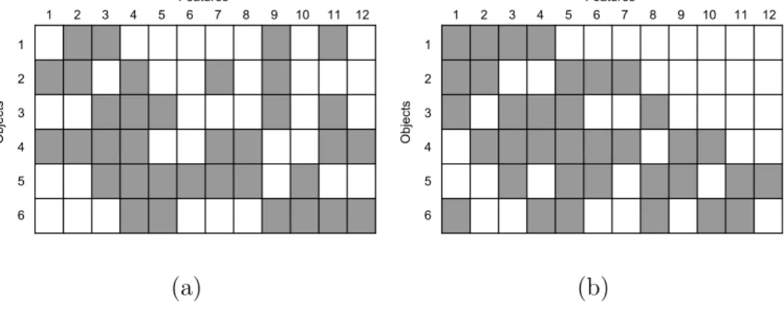
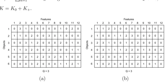
1.1 An example of binary matrix representation of feature alloca-tion. A shaded rectangle indicates the corresponding matrix element znk = 1. The binary matrix on (a) is transformed into the left-ordered binary matrix on (b) by the function lof(_·). . 22 1.2 An example of (Q+ 1)-nary matrix with Q = 3. The matrix

on (a) is transformed into the left-ordered matrix on (b) by the function lof(·). . . 30 2.1 (a) Illustration of tumor evolution, emergence of subclones and

their population frequencies. (b) Illustration of the subclone structure matrix Z. Right panel: A subclone is represented by one column of Z. Each element of a column represents the subclonal genotypes for a mutation pair. For example, the geno-types for mutation pair 2 in subclone 1 is ((0, 1), (1, 1)), which is shown in detail on the left panel. Left panel: The reference genome for mutation pair 2 is (G, T) and the corresponding genotype of subclone 1 is ((G, C), (A, C)), which gives rise to

z21 = ((0,1),(1,1)). (c) Illustration of paired-end reads data

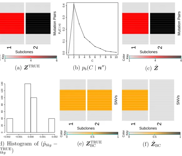
for a mutation pair. Shown are four short reads mapped to mutation pair k in sample t. Some reads are mapped to both loci of the mutation pair, and others are mapped to only one of the two loci. The two ends of the same read are marked with opposing arrows in purple and orange. . . 45 2.2 Simulation 1. Simulation truth ZTRUE (a, e), and posterior

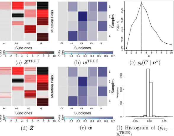
inference under PairClone (b, c, d) and under BayClone (f). . 62 2.3 Simulation 1. Posterior inference under PyClone. . . 63 2.4 Simulation 2. Simulation truth ZTRUE and wTRUE (a, b), and

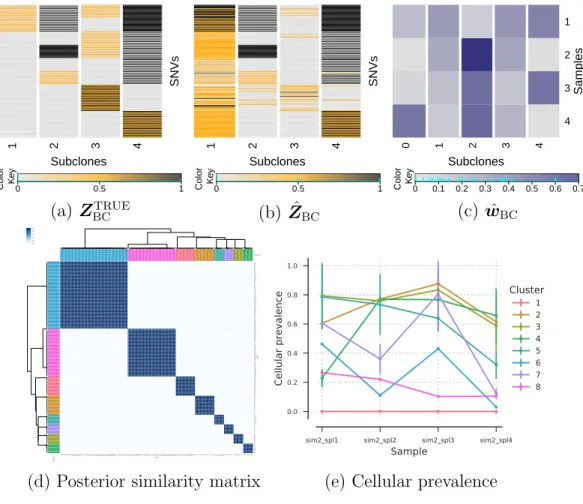
posterior inference under PairClone (c, d, e, f). . . 66 2.5 Simulation 2. Posterior inference under BayClone (a, b, c) and

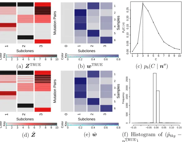
PyClone (d, e). . . 67 2.6 Simulation 3. Simulation truth ZTRUE and wTRUE (a, b), and

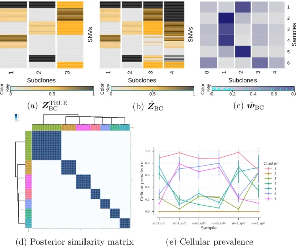
posterior inference under PairClone (c, d, e, f). . . 69 2.7 Simulation 3. Posterior inference under BayClone (a, b, c) and

(16)

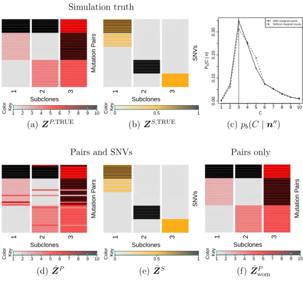
2.8 Summary of simulation results using additional marginal read counts. Simulation truthZP,TRUEandZS,TRUE (a, b), posterior inference with marginal read counts incorporated (c, d, e), and posterior inference without marginal read counts (c, f). . . 73 2.9 Summary of simulation results with tumor purity incorporated. 74 2.10 Lung cancer. Posterior inference under PairClone. . . 79 2.11 Lung cancer. Posterior inference under BayClone (a, b) and

PyClone (c, d). . . 81 2.12 Lung cancer. Posterior inference under PyClone using 1800

SNVs. PyClone inferred 34 clusters with two major clusters (olive and green) and many small noisy clusters (other colors). 82 3.1 Short reads data from mutation pairs using NGS. Here stki

de-notes the i-th read for thek-th mutation pair in samplet. Each stkiis a 2-dimensional vector which corresponds to the two prox-imal SNVs in the mutation pair, and each component of the vector takes values 0, 1 or – representing wild type, variant or missing genotype, respectively. . . 88 3.2 Schematic of subclonal evolution and subclone structure. Panel

(a) shows the evolution of subclones over time. Panel (b) shows the subclonal structure at T4 with genotypes Z, cellular

pro-portions w and parent vector _T. For each mutation pair k and subclonec, the entryzkc ofZ is a 2×2 matrix corresponding to the arrangement in the figure in panel (a), that is, with alleles in the two columns, and SNVs in the rows. . . 93 3.3 Simulation 1. Simulation truth Z (a) and phylogeny (d), and

posterior inference under PairCloneTree (b, c, e). . . 106 3.4 Simulation 1. Simulation truth ZCloe (a), and posterior

infer-ence under Cloe (b) and PhyloWGS (c). . . 110 3.5 Simulation 2. Simulation truthZ (a),w(b) and phylogeny (c),

and posterior inference under PairCloneTree (c, d, e) and Cloe (f). . . 112 3.6 Posterior inference with PairCloneTree for lung cancer data set. 114 3.7 Posterior inference with Cloe (a, b) and PhyloWGS (c) for lung

cancer data set. . . 116 4.1 Trajectories of individual responses (dashed black lines) and

mean responses (thick red lines) over time for the active control, placebo and test drug arms. . . 124

(17)

4.2 Cumulative dropout rates (top) and observed-data means (bot-tom) over time obtained from the model versus the ones ob-tained from the empirical distribution. The solid red line rep-resents the empirical values, black dots represent the posterior means, red dashed error bars represent frequentist 95% confi-dence intervals, and black solid error bars represent the model’s 95% credible intervals. . . 149 4.3 Change from baseline treatment effect improvements of the test

drug (top) and active drug (bottom) over placebo over time. Smaller values indicate more improvement compared to place-bo. The dividing line within the boxes represents the posterior mean, the bottom and top of the boxes are the first and third quartiles, and the ends of the whiskers show the 0.025 and 0.975 quantiles. . . 152 4.4 Contour plots showing inferences on treatment effect

improve-ments r1 −r3 (left) and r2 −r3 (right) for different choices of

the sensitivity parameters along the [0,1] grid. The colors rep-resent posterior means ofrx−r3, where a deeper color indicates

more improvement compared to placebo. The black lines show posterior probabilities of rx−r3 <0. . . 154

A.1 Path plot of ˆC with different test sample sizes for three sim-ulations. The true number of subclones are 2, 4, and 3 for simulations 1, 2, and 3, respectively. . . 168 A.2 Convergence check for Simulation 2. . . 171

(18)

Chapter 1 Introduction

1.1 Overview

This dissertation develops nonparametric Bayesian models, correspond-ing Markov chain Monte Carlo (MCMC) algorithms, and applications for biomedical data analysis. Chapters 2 and 3 are about applications to genomic data analysis, and Chapter 4 discusses applications to longitudinal missing data analysis. Nonparametric Bayesian methods provide flexible and highly adaptable approaches for statistical inference. In applications with biostatis-tics data such methods can often better address biological research problems than more restrictive parametric methods.

In Chapter 2, we talk about inference on tumor heterogeneity. Dur-ing tumor growth, tumor cells acquire somatic mutations that allow them to gain advantages compared to normal cells. As a result, tumor cell populations are typically heterogeneous consisting of multiple subpopulations with unique genomes, characterized by different subsets of mutations. This is known as tu-mor heterogeneity. The homogeneous subpopulations are known as subclones and are an important target in precision medicine. We propose a Bayesian feature allocation model to reconstruct tumor subclones using next-generation

(19)

sequencing (NGS) data. The key innovation is the use of (phased) pairs of proximal single nucleotide variants (SNVs) for the subclone reconstruction. We utilize parallel tempering to achieve a better mixing Markov chain with highly multi-modal posterior distributions. We also develop trans-dimensional MCMC algorithms with transition probabilities that are based on splitting the data into training and test data sets to efficiently implement trans-dimensional MCMC sampling. Through simulation studies we show that inference under our model outperforms models using only marginal SNVs by recovering the number of subclones as well as their structures more accurately. This is the case despite significantly smaller number of phased pairs than the number of marginal SNVs. Estimating our model for four lung cancer tissue samples, we successfully infer their subclone structures. For this work, I collaborate with Peter Mueller (The University of Texas at Austin), Subhajit Sengupta (NorthShore University HealthSystem) and Yuan Ji (NorthShore University HealthSystem and The University of Chicago).

In Chapter 3, we address another important aspect of statistical infer-ence for tumor heterogeneity, aiming to recover the phylogenetic relationship of subclones. Such inference can significantly enrich our understanding of subclone evolution and cancer development. We develop a tree-based feature allocation model which explicitly models dependence structure among sub-clones. That is, in contrast to commonly used feature allocation models, we allow the latent features to be dependent, using a tree structure to introduce dependence. In the application to inference for tumor heterogeneity this tree

(20)

structure is interpreted as a phylogenetic tree of tumor cell subpopulations. We adapt our MCMC sampling techniques to efficiently search the tree space. We analyze a lung cancer data set and infer the underlying evolutionary pro-cess. For this work, I collaborate with Subhajit Sengupta, Peter Mueller and Yuan Ji.

In Chapter 4, we model missing data in longitudinal studies. In lon-gitudinal clinical studies, the research objective is often to make inference on a subject’s full data response conditional on covariates that are of primary interest; for example, to calculate the treatment effect of a test drug at the end of a study. The vector of responses for a research subject is often incom-plete due to dropout. Dropout is typically non-ignorable and in such cases the joint distribution of the full data response and missingness needs to be modeled. In addition to the covariates that are of primary interest, we would often have access to some auxiliary covariates (often collected at baseline) that are not desired in the model for the primary research question. Such variables can often provide information about the missing responses and missing data mechanism. In this setting, auxiliary covariates should be incorporated in the joint model as well, and we should proceed with inference unconditional on these auxiliary covariates. As a result, we consider a joint model for the full data response, missingness and auxiliary covariates. In particular, we specify a nonparametric Bayesian model for the observed data via Gaussian process priors and Bayesian additive regression trees. These model specifications al-low us to capture non-linear and non-additive effects, in contrast to existing

(21)

parametric methods. We then separately specify the conditional distribution of the missing data response given the observed data response, missingness and auxiliary covariates (i.e. the extrapolation distribution) using identifying restrictions. We introduce meaningful sensitivity parameters that allow for a simple sensitivity analysis. Informative priors on those sensitivity parameters can be elicited from subject-matter experts. We use Monte Carlo integration to compute the full data estimands. Our methodology is motivated by, and applied to, data from a clinical trial on treatments for schizophrenia. For this work, I collaborate with Michael Daniels (The University of Texas at Austin). The remainder of this chapter is organized as follows, Section 1.2 con-tains basics of Bayesian inference and Bayesian nonparametrics. Sections 1.3, 1.4 and 1.5 present three classes of statistical models, discuss how nonpara-metric Bayesian methods can be used, and demonstrate applications related to succeeding chapters. These models include latent class models, latent feature models and regression.

1.2 Bayesian Nonparametrics

Bayesian Inference. By way of introducing notation, we briefly review the

setup of Bayesian inference. Bayesian inference, named for Thomas Bayes, is a particular approach to statistical inference. Let y denote the observed

data, θ denote the unobserved parameters of interest, and ˜y denote unknown but potentially observable quantities (such as a data point that is not yet observed) of interest. In the Bayesian framework, we update our belief on the

(22)

unobserved parameters according to evidences in the observed data based on Bayes’ rule:

p(θ _|y) = p(y|θ)p(θ)

p(y) . (1.1)

In equation (1.1), p(θ) is called the prior distribution, p(y | θ) is called the

sampling distribution (when regarded as a function of y with fixed θ) or the

likelihood (when regarded as a function of θ with fixed y). The denominator

p(y) is the marginal distribution of y, which is calculated by p(y) = R

p(y _| θ)p(θ)dθ. Inference onθ is given by theposterior distribution p(θ_|y). We can then make inference on ˜y based on the posterior predictive distribution

p(˜y |y) =

Z

p(˜y|θ)p(θ |y)dθ.

Bayesian statistical inference is stated in terms of probability statements con-ditional on the observed values of y. For a review of Bayesian statistics, see, for example, Gelman et al. (2014) or Hoff (2009).

Exchangeability. Exchangeabilityplays an important role in statistics.

Sup-pose we have N random variables (which can be data points or parameters) with a joint distribution p(y1, . . . , yN). The random variables are called

ex-changeable if their joint distribution is invariant to permutation. Let [N] = {1, . . . , N_} and denote by σ : [N] _→ [N] a permutation of [N]. (Finite) exchangeability states that

y1, . . . , yN

d

(23)

for any σ, where = means equal in distribution. Furthermore, an infinited sequence of random variablesy1, y2, . . . is called infinitely exchangeable if

y1, y2, . . .

d

=yσ(1), yσ(2), . . . ,

where σ : _N _→ _N is a finite permutation. That is, for some finite value Nσ, σ(n) = n for all N > Nσ.

The importance of exchangeability is due to de Finetti’s theorem (De Finet-ti, 1931, Hewitt and Savage, 1955, De FinetFinet-ti, 1974), which states that 1 _if

y1, y2, . . . are infinitely exchangeable random variables, their joint distribution

can be expressed as a mixture of independent and identical distributions p(y1, . . . , yN) = Z N Y i=1 p(yi |θ) ! p(θ)dθ. (1.2) The theorem can be rephrased from a more general perspective2_{. If} _y

1, y2, . . .

are infinitely exchangeable, there exists a random distributionF such that the sequence is composed of i.i.d. draws from it,

p(y1, . . . , yN) =

Z N Y

i=1

F(yi)dp(F). (1.3) That is,θ in Equation (1.2) can be interpreted as indexing a probability mea-sure F, or θ can even be the probability measure F itself.

1_{This is a rephrased simpler version from Gelman et al. (2014). The original version is}

a statement about probability measure. De Finetti’s original paper De Finetti (1931) is for the case of binary random variables, and Hewitt and Savage (1955) extended it to any real valued random variables.

(24)

Bayesian Nonparametrics. A model is called parametric if it only has a finite (and usually small) number of parameters, i.e. θ lives in a finite dimen-sional space. In contrast, a nonparametric model has a potentially infinite number of parameters, i.e. θ or F are in an infinite dimensional space. Thus, nonparametric Bayesian inference requires constructing probability tions on an infinite dimensional parameter space. Such probability distribu-tions are calledstochastic processes with sample paths in the parameter space. Nonparametric Bayesian methods avoid the often restrictive assumptions of parametric models and provide flexible and highly adaptable approaches for statistical modeling. Reviews of Bayesian nonparametrics include Hjort et al. (2010), Ghosh and Ramamoorthi (2003), M¨uller et al. (2015), Walker et al. (1999), M¨uller and Quintana (2004), Orbanz and Teh (2011), Gershman and Blei (2012) and Orbanz (2014)3_.

Nonparametric Bayesian approaches have been widely used in many statistical inference problems, including density estimation, clustering, feature allocation, regression, classification, and graphical models. In the next sec-tions, we give examples to show how Bayesian nonparametric approaches can be applied to address those important problems.

3_{Hjort et al. (2010) includes a set of introductory and overview papers, Ghosh and}

Ramamoorthi (2003) focuses on posterior convergence, and M¨uller et al. (2015) has more discussion on data analysis problems.

(25)

1.3 Latent Class Models

Suppose we have N objects y1, . . . , yN. In a latent class model (for

a review, see Griffiths and Ghahramani, 2011), each object yn belongs to a latent class cn =k, k = 1, . . . , K, where K is the number of possible classes, and K = _∞ is allowed. When K = _∞, the model has an infinite number of classes and thus has an infinite number of parameters. In this case, the model is nonparametric. We are interested in how the classes are related to the objects, p(y _| c), and the distribution over class assignments, p(c). For p(y_|c), we assume conditional independence,

p(y _|c) = N Y n=1 p(yn _|cn), p(yn|cn=k, µ∗k) =G(· |µ∗k). (1.4) That is, for an object belonging to classk, we assume it has a distribution G with parameterµ∗

k. We then put some prior distributionF0 on theµ∗k’s, µ∗₁, . . . , µ∗_K iid∼F0. (1.5)

Next, we specify p(c). Specifying p(c) is equivalent to defining a dis-tribution on a random partition of the index set [N] := _{1,2, . . . , N_}. The formal definition of random partition follows in Section 1.3.1. The equivalence can be seen by noticing that the unique values of c correspond to a partition of [N], fN ={A1, . . . , AK}, with n∈Ak if cn=k, and vice versa.

(26)

1.3.1 Random Partition

We briefly summarize the definition of random partitions as given in Broderick, Jordan, and Pitman (2013). See there for more details and discus-sion. Let [N] := {1,2, . . . , N} denote the index set of N objects. A partition

fN of [N] is a collection of mutually exclusive, exhaustive, nonempty subsets A1, . . . , AK of [N] called blocks. LetfN ={A1, . . . , AK}, whereK is the

num-ber of blocks. Here N = ∞ is allowed, in which case the index set becomes N={1,2,3, . . .}, andK =∞ is also allowed.

Let _FN be the space of all partitions of [N]. A random partition FN of [N] is a random element of _FN. The probability p(FN = fN) is called the partition probability function ofFN.

Exchangeability of a random partition can be defined as follows. Let σ :N→Nbe a finite permutation. That is, for some finite valueNσ,σ(n) =n for all N > Nσ. Furthermore, for any block A ⊂ N, denote the permutation applied to the block as σ(A) := {σ(n) : n ∈ A}. For any partition ΠN, denote the permutation applied to the partition as σ(ΠN) := {σ(A) : A ∈ ΠN}. A random partition ΠN is called exchangeable if ΠN =d σ(ΠN) for every permutation of [N]. The importance of exchangeability has been stated in Section 1.2.

1.3.2 Chinese Restaurant Process

The Chinese restaurant process (CRP) defines an exchangeable random partition. The CRP can be derived in multiple ways, such as from the Dirichlet

(27)

process (Blackwell and MacQueen, 1973), or by taking limit of a finite mixture model (Green and Richardson, 2001, Neal, 1992, 2000). We take the latter approach, following Griffiths and Ghahramani (2011).

A Finite Mixture Model. We assume object i belongs to class k with

probabilityπk,

p(cn =k _|πk) =πk.

Note that the distribution of c always induces a distribution on a random partition of [N]. In the above case, the assignment of an object to a class is independent of the assignments of the other objects conditional onπ, and the latent class model is called amixture model. To complete the model, we put a symmetric Dirichlet distribution prior on (π1, . . . , πK),

(π1, . . . , πK)∼Dir(α/K, . . . , α/K),

πk ≥0 and PK

k=1πk= 1.

Integrating out the πk’s, the marginal distribution of c is p(c) = QK k=1Γ(mk+Kα) Γ _KαK Γ(α) Γ(N +α), (1.6) wheremk=PN

n=1I(cn =k) is the number of objects assigned to classk. This

distribution is exchangeable, since it only depends on the counts and does not depend on the ordering of objects.

(28)

Equivalence Classes. A partitioncincludes an ordering of theK blocks by increasing labels k = 1, . . . , K. In many applications, we are only interested in the division of objects, and the ordering of the blocks does not matter. For example, f3 = {{1},{2,3}} and f30 = {{2,3},{1}} correspond to the same

division of objects, where the only difference is the choice of labels of the blocks. If the order of the blocks is not identifiable, it is helpful to define an equivalence class of assignment vectors, denoted by [c], with two assignment vectorscandc0 belonging to the same equivalence class if they imply the same division of objects.

We therefore focus on the equivalence classes [c]. LetK+be the number

of classes for whichmk >0, andK0 be the number of classes for whichmk= 0,

soK = K0+K+. The cardinality of [c] is (K!/K0!). Taking the summation

over all assignment vectors that belong to the same equivalence class, and expanding (1.6), we obtain p([c]) = X c∈[c] p(c) = K! K0! α K K+ _YK+ k=1 mk−1 Y j=1 j+ α K ! Γ(α) Γ(N +α). (1.7)

Taking the Infinite Limit. When the number of classes K → ∞, taking

the limit in Equation (1.7), we get lim K→∞p([c]) =α K+ K+ Y k=1 (mk₋1)! ! Γ(α) Γ(N +α). (1.8)

(29)

See details in Griffiths and Ghahramani (2011). Note that this distribution is still exchangeable, just as in the finite case.

Chinese Restaurant Analogy. The Chinese restaurant analogy (Aldous,

1985) 4 _{comes from the fact that the distribution in Equation (1.8) can be}

described by a Chinese restaurant metaphor. Let theN objects be customers in a restaurant, and the K classes be tables at which they sit, K = ∞. The customers enter the restaurant one by one, and each chooses a table at random. At time 1, the first customer comes in and chooses the first table to sit. At time n, the n-th customer comes in, chooses an occupied table with probability proportional to the number of customers sitting at that table, or the first unoccupied table with probability proportional to α, n = 2, . . . , N. The customers and tables form a partition of c, if we treat the tables as partition blocks. Denote bycn =k the event that customer n sits at table k, mk the number of customers sitting at table k after time n ₋1, and K+ =

max_{c1, . . . , cn−1} . Mathematically, the CRP can be written as

cn|c1, . . . , cn−1 = ( k, w. pr. mk α+n−1, for k ≤K+; K++ 1, w. pr. _α₊α_n₋₁, (1.9) for n = 1, . . . , N. The probability of a partition of c given by Equation (1.9) is identical to what given in Equation (1.8).

Dirichlet Process. The CRP defines an exchangeable random partition of

[N]. We can further extend he model by assigning each table k a value µ∗

k,

(30)

with µ∗

k generated from some fixed distribution F0. We then assign customer

n a value µn =µ∗

k if the customer sits at table k. The predictive distribution ofµn given the values µ1, . . . , µn−1 of the firstn−1 customers is

µn_|µ1, . . . , µn−1 = ( µ∗ k, w. pr. α+mnk−1, for k ≤K+; µ∗ K++1 ∼F0, w. pr. α α+n−1. (1.10) It can be shown that the random sequenceµ1, µ2, . . .is infinitely exchangeable.

By Equation (1.3), there exists a random distributionF such thatµn |F iid∼ F andF ∼υ. Here υ is a prior over the random distributionF, which is known as the Dirichlet process (DP) (Ferguson, 1973). We denote by DP(α, F0) a

DP with concentration parameterαand base distributionF0. Equation (1.10)

is also called the P´olya urn representation (Blackwell and MacQueen, 1973) of the DP. Using the notion of DP, we can re-parameterize Equations (1.4), (1.5) and (1.9) with a hierarchical model

yn|µn ∼G(· |µn) µn_|F _∼F

F |α, F0 ∼ DP(α, F0)

(1.11)

The model (1.11) is called a Dirichlet process mixture (DPM) model.

The DP is probably the most popular nonparametric Bayesian mod-el. Discussions and extensions of the DP include Blackwell (1973), Blackwell and MacQueen (1973), Antoniak (1974), Lo et al. (1984), Sethuraman (1994), Pitman and Yor (1997), MacEachern (2000), M¨uller et al. (2004), Teh et al. (2006), Rodriguez et al. (2008), Lijoi and Pr¨unster (2010), Adams et al. (2010), Teh (2011), De Blasi et al. (2015), where Sethuraman (1994) proposes the

(31)

stick-breaking construction of the DP, Pitman and Yor (1997) extend the DP to the Pitman-Yor process, MacEachern (2000) proposes the dependent DP, Teh et al. (2006) develop the hierarchical DP, and Rodriguez et al. (2008) de-velop the nested DP. Literature about posterior inference methods for the DP includes West et al. (1994), Escobar and West (1995), MacEachern and M¨uller (1998), Neal (2000), Rasmussen (2000), Ishwaran and James (2001), Jain and Neal (2004), and Blei and Jordan (2006).

1.3.3 Related Applications

Latent class models, in particular, the DPM model and its variations, have been extensively used in many data analysis problems. We highlight their applications to inference for tumor heterogeneity and inference for missing data because of the relevance to the following chapters.

Inference for Tumor Heterogeneity. Tumor cell populations are

typi-cally heterogeneous consisting of multiple homogeneous subpopulations with unique genomes. Such subpopulations are known as subclones. Our goal is reconstructing such subclones from next-generation sequencing (NGS) data (Mardis, 2008). See more details in Chapters 2 and 3. One approach to this problem is to model the observed read count data using a latent class model. This approach is taken by PyClone (Roth et al., 2014) and PhyloWGS (Jiao et al., 2014, Deshwar et al., 2015). Tumor evolution is a complex process in-volving many biological details, such as tumor purity, copy number variations

(32)

and tumor phylogeny. Also, NGS data are subject to sequencing error and are often overdispersed. For simplicity of illustration we consider only one pure tumor tissue sample, ignore all the complexities mentioned above and also ignore the zygosity of the mutation sites. For detailed discussions see, for example, Roth et al. (2014), Jiao et al. (2014), Deshwar et al. (2015) and Chapters 2 and 3.

Consider S single nucleotide variants (SNVs). Here SNVs refer to the loci of the nucleotides (base pairs) for which we record variants. Variants are defined relative to some reference genome. The SNVs are the objects in the latent class model. In an NGS experiment, DNA fragments are first produced by extracting the DNA molecules from the cells in a tumor sample. The fragments are then sequenced using short reads. The short reads are mapped to the reference genome, and counts are recorded for each locus (i.e. base pair). In the end, for each SNV locus s(s= 1, . . . , S), denote byNs and ns the total number of reads and number of variant reads covering the locus, respectively. The total number of reads Ns is usually treated as a fixed number. PyClone uses a DPM model for ns,

ns |ps∼Binom(Ns;ps), ps_|F _∼F,

F |α, F0 ∼ DP(α, F0),

where the base distribution F0 is chosen to be Unif(0,1). Here ps is known as

(33)

harbour-ing a mutation. The DP prior for F allows multiple mutations to share the same cellular prevalence. The critical step towards subclone reconstruction is the following. Mutations having the same cellular prevalence are thought of having occurred at the same point in the clonal phylogeny. Thus, latent classes of mutations can be used as markers of subclone populations (Roth et al., 2014). We note that this is essentially an application of latent class models toclustering. PhyloWGS, on the other hand, uses the tree-structured stick breaking process (TSSB) (Adams et al., 2010) as the prior for F,

F _|α, γ, F0 ∼TSSB(α, γ, F0),

which allows it to infer tumor phylogeny.

One restriction of the latent class model is that each object can only belong to one class. In the tumor heterogeneity application, this restriction implies that each mutation can only occur once in the clonal phylogeny. There-fore, subclone reconstruction methods based on latent class models usually rely on the infinite site assumption (ISA) (Kimura, 1969), which can be summa-rized as (Roth et al., 2014)

1. Subclone populations follow a perfect phylogeny. That is, no SNV site mutates more than once in its evolutionary history;

2. Subclone populations follow a persistent phylogeny. That is, mutations do not disappear or revert.

However, ISA is not necessarily valid, in which case we should model the observed read count data using latent feature models. See Section 1.4.5.

(34)

Inference for Missing Data. Missing data are very common in real stud-ies. Missingness is typically non-ignorable (Rubin, 1976, Little and Rubin, 2014), and in such cases the joint distribution of the full data response and missingness needs to be modeled. We focus on the missing outcome case. See Linero and Daniels (2017) for a general review of Bayesian nonparametric ap-proach to missing outcome data. LetYij denote the outcome that was planned to be collected for subjectiat timej, andRij be the missingness indicator with Rij = 1 or 0 accordingly as Yij is observed or not, i= 1, . . . , N, j = 1, . . . , J. LetXi denote the covariates that are of primary interest to the study. In longi-tudinal clinical trial setting,Xi is usually an indicator of treatment. We often treat Xi as fixed and do not proceed with inference on it. The full data for subject i are (Yi,Ri,Xi). The observed data for subject iare (Yi,obs,Ri,Xi),

where Y_i,_obs = (Yij | j : Rij = 1). We assume (Yi,Ri | Xi) iid

∼ p(y,r _| x). We stratify the model by x and suppress the conditional on x hereafter to simplify notation. The extrapolation factorization (Daniels and Hogan, 2008) factorizes

p(y,r) = p(ymis |yobs,r)p(yobs,r).

The observed data distribution p(yobs,r) is identified by the observed data,

while the extrapolation distribution p(ymis | yobs,r) is not. Identifying the

extrapolation distribution relies on untestable assumptions such as parametric models for the full data distribution or identifying restrictions. See Chapter 4 or Linero and Daniels (2017).

(35)

For current discussion, we focus on specifying p(yobs,r). One way of

specifying p(yobs,r) is specifying p(y,r), and set

p(yobs,r) =

Z

p(y,r)dymis.

This is known as the working model idea (Linero and Daniels, 2015, Linero, 2017, Linero and Daniels, 2017). Linero and Daniels (2017) discuss a Bayesian nonparametric framework for modeling a complex joint distribution of outcome and missingness, which sets

p(y,r) = K

X

k=1

πkG(· |µk). (1.12)

Equation (1.12) is another way of writing a latent class model

Y_i,R_i _|ci =k,µk ∼G(· |µk), p(ci =k|πk) =πk.

When K =∞, mixture models of the form (1.12) can approximate any joint distribution for (Yi,Ri) (subject to technical constraints). We note that this is essentially an application of latent class models to density estimation.

Linero and Daniels (2017) use a model of the form (1.12) to analyze data from the Breast Cancer Prevention Trial. In this trial, Yij = 1 or 0 represent subject i is depressed or not at time j. They model

p(y,r) = ∞ X k=1 πk ( _J Y j=1 γrj kj(1−γkj) 1−rj ) ( _J Y j=1 βyj kj(1−βkj) 1−rj ) .

Linero and Daniels (2015) discussion is another example of applying latent class models to inference for missing data. They analyze data from an

(36)

acute schizophrenia clinical trial, where the outcome Yij is a continuous vari-able called the positive and negative syndrome scale (PANSS) score. Missing-ness is monotone in this application. That means, if Yij was unobserved then Yi,j+1 was also unobserved. LetSi denote the dropout time, i.e. ifSi =j then Yij was observed butYi,j+1 was not. For monotone missingness,S captures all

the information about missingness. Denote byY¯ij = (Yi1, . . . , Yij) the history

of outcomes through the firstj times. They model p(y, s) = ∞ X k=1 πkf(y_|µk,Σk)g(s |y,ζk,γk), with f(y_|µ,Σ) =N(y;µ,Σ), logit[g(S =j _|S _≥j,y,ζ,γ)] =ζj+γ_jTy¯j.

1.4 Latent Feature Models

Suppose we haveN objects,y1, . . . , yN. In alatent feature model (for a

review, see Griffiths and Ghahramani, 2011), each object yn is represented by a vector of latent feature values dn = (dn1, . . . , dnK), where K is the number

of features. Similar to the latent class model case,K =_∞is allowed, in which case the model is nonparametric. Examples of latent feature models include probabilistic principle component analysis (Tipping and Bishop, 1999) and factor analysis (Roweis and Ghahramani, 1999). We focus on the case that there is no upper bound on the number of features.

(37)

We can break the vector dn into two components: a binary vector zn with znk = 1 if object n has feature k and 0 otherwise, and a second vector

v = (v1, . . . , vK) indicating the value of each feature. The vector dn can be expressed as the elementwise product of zn and v, i.e.

dnk =znkvk, k = 1, . . . , K. (1.13) Let D = (d1, . . . ,dN)T and Z = (z1, . . . ,zN)T denote N ×K matrices with columns dn and zn, respectively. We are interested in how the feature values are related to the data, p(y _| D), and the distribution over feature values, p(D). For p(y_|D), we generally assume conditional independence

p(y _|D) = N Y n=1 p(yn_|dn), p(yn |dn)∼G(· |dn). (1.14) The distribution p(D) can be broken into two components, with p(D) being determined by p(Z) and p(v). We assume an independent prior onv,

v1, . . . , vK iid∼F0.

We then focus on defining a prior on Z. Specifying p(Z) is equivalent to defining a distribution on arandom feature allocation of the index set [N]. The formal definition of random feature allocation follows in Section 1.4.1. The equivalence can be seen by noticing that the values ofZ correspond to a feature allocation fN = {A1, . . . , AK}, with n ∈ Ak if znk = 1 and n /∈ Ak if

(38)

1.4.1 Random Feature Allocation

We briefly summarize the definition of random feature allocations from Broderick, Jordan, and Pitman (2013). See there for more details and discus-sion. Feature allocations could be seen as a generalization of partitions which relaxes the restriction to mutually exclusive and exhaustive subsets. Consider an index set [N]. A feature allocation fN of [N] is a multiset of non-empty subsets of [N] called features, such that no index n belongs to infinitely many features. Denote by fN = _{A1, . . . , AK}, where K is the number of features.

Here N =_∞and K =_∞are allowed. For example, a feature allocation of [6] is f6 ={{1,4},{1,3,6},{4},{4},{4}}.

LetFN be the space of all feature allocations of [N]. Arandom feature

allocation FN of [N] is a random element of FN.

Let σ : N → N be a finite permutation. That is, for some finite value Nσ, σ(n) = n for all N > Nσ. Furthermore, for any feature A ⊂ N, denote the permutation applied to the feature as σ(A) := _{σ(n) : n _∈ A_}. For any feature allocationFN, denote the permutation applied to the feature allocation asσ(FN) := {σ(A) :A∈FN}. Let FN be a random feature allocation of [N]. A random feature allocationFN is calledexchangeable ifFN =d σ(FN) for every permutation of [N].

Matrix Representation. Suppose N objects and K features are present.

A feature allocation can be represented by aN_×K binary matrix, denoted by

(39)

features. Each elementznk, n = 1, . . . , N,k = 1, . . . , K, is a binary indicator, whereznk = 0 or 1 indicates indexnbelongs or does not belong to featurek, i.e. n /_∈Ak orn_∈Ak, respectively. For example, Figure 1.1(a) shows a feature al-location of [6] with 12 features,f6 ={{2,4},{1,2,4},{1,3,4,5},{2,3,4,5,6},

{3,5,6_},_{5_}, _{2,4,5_},_{4,5_},_{1,2,3,6_}, _{5,6_}, _{1,3,4,6_},_{4,6_}}. Features Objects 1 2 3 4 5 6 7 8 9 10 11 12 1 2 3 4 5 6 (a) Features Objects 1 2 3 4 5 6 7 8 9 10 11 12 1 2 3 4 5 6 (b)

Figure 1.1: An example of binary matrix representation of feature allocation. A shaded rectangle indicates the corresponding matrix element znk = 1. The binary matrix on (a) is transformed into the left-ordered binary matrix on (b) by the functionlof(_·).

1.4.2 Indian Buffet Process

The Indian buffet process (IBP) (Griffiths and Ghahramani, 2006, 2011)) is a popular example of an exchangeable random feature allocation. Using the matrix representation of feature allocation, the IBP defines a distribution on binary matrices (with an unbounded random number of columns).

(40)

A Finite Feature Model. The IBP can be defined as the limit of a finite feature model. Suppose we have N objects and K features. We use a binary variableznk to indicate object n has feature k, thus znk form a binary N _×K matrix Z. We assume that each object possesses feature k with probability πk, and the features are independent. Furthermore, beta distribution priors are put onπk’s. That is,

znk |πk∼Bernulli(πk); πk_∼Beta(α/K,1).

Integrating out the πk’s, the marginal distribution of Z is p(Z) = K Y k=1 α KΓ(mk+ α K)Γ(N −mk+ 1) Γ(N + 1 +_Kα) , where mk = PN

n=1znk is the number of objects possessing feature k. This

distribution is exchangeable, since it only depends on the counts and does not depend on the ordering of the objects.

Left-ordered Constraint and Equivalence Classes. A feature allocation

indicates an ordering of theK features. In many applications, the ordering of the features is not identifiable. When the labels of the features are arbitrary, it is helpful to define an equivalence class of binary matrices, denoted by [Z]. We first introduce an order constraint on binary matrices called the

left-ordered constraint. For a binary matrix Z, its corresponding left-ordered

(41)

from left to right by the magnitude of the binary number expressed by that column, taking the first row as the most significant bit. For example, Figure 1.1(b) shows the corresponding left-ordered binary matrix of Figure 1.1(a). In the first row of the left-ordered matrix, the columns for which z1k = 1 are grouped at the left. In the second row, the columns for which z2k = 1 are grouped at the left of the sets for which z1k = 1. This grouping structure persists throughout the matrix.

We can then define equivalence classes with respect to the function lof(_·). This function maps binary matrices to left-ordered binary matrices, as described before. The function lof(·) is many-to-one: many binary matri-ces reduce to the same left-ordered form, and there is a unique left-ordered form for every binary matrix. Any two binary matrices Y and Z are lof(·) equivalent if lof(Y) =lof(Z). In models where feature order is not identifi-able, performing inference at the level oflof-equivalence classes is appropriate. The probability of a particularlof-equivalence class of binary matrices [Z] is p([Z]) =P

Z∈[Z]p(Z).

The matrix left-ordered form motivates the following definition. The

history of feature k at object n is defined to be (z1k, . . . , z(n−1)k). When n

is not specified, history refers to the full history of feature k, (z1k, ..., zN k).

The histories of features are individuated using the decimal equivalent of the binary numbers corresponding to the column entries. For example, at object 3, features can have one of four histories: 0, corresponding to a feature with no previous assignments, 1, being a feature for which z2k = 1 but z1k = 0, 2,

(42)

being a feature for whichz1k= 1 butz2k = 0, and 3, being a feature possessed by both previous objects were assigned. The number of features possessing the history h is denoted by Kh, with K0 being the number of features for which

mk = 0 andK+ =P2

N₋₁

h=1 Kh being the number of features for whichmk>0,

so K = K0+K+. The function lof thus places the columns of a matrix in

ascending order of their histories.

Using the notion above, the cardinality of [Z] is K!/Q2N−1

h=0 Kh! . Thus, p([Z]) = K! Q2N−1 h=0 Kh! · K Y k=1 α KΓ(mk+ α K)Γ(N −mk+ 1) Γ(N + 1 + α K) . (1.15)

Taking the Infinite Limit. Taking the limitK _{→ ∞}in Equation (1.15),

lim K→∞p([Z]) = αK+ Q2N−1 h=1 Kh! ·exp{−αHN} · K+ Y k=1 (N −mk)!(mk−1)! N! , (1.16)

where HN is the N-th harmonic number, HN = PN

j=11/j. See Griffiths and

Ghahramani (2011) for details. This distribution is still exchangeable. In practice, we usually drop all columns with all zeros, since they corresponds to the features that no object possesses, and it should not be included in the feature allocation as features are non-empty sets. It can be proved that we can obtain a matrix with finite columns with probability 1 by deleting the columns with all zeros.

Indian Buffet Analogy. The probability distribution defined in Equation

(43)

as the IBP. Think about an Indian buffet where customers (objects) choose dishes (features). In the buffet, N customers enter one after another, and each customer encounters infinitely many dishes arranged in a line. The first customer starts at the left of the buffet and takes a serving from each dish, stopping after a Poisson(α) number of dishes. Then-th customer moves along the buffet, sampling dishes in proportion to their popularity, serving himself with probability mk/n, where mk is the number of previous customers who have sampled a dish. Having reached the end of all previously sampled dishes, the n-th customer then tries a Poisson(α/n) number of new dishes. We use a binary matrixZ with N rows and infinitely many columns to indicate which customers chose which dishes, where znk = 1 if the n-th customer sampled the k-th dish. The matrices produced by this process are generally not in left-ordered form, and customers are not exchangeable under this distribution. However, if we only record thelof-equivalence classes of the matrices generated by this process, one obtains the exchangeable distribution p([Z]) given by Equation (1.16).

Beta Process. Similar to the relationship between the DP and the CRP,

the de Finetti’s measure underlying the exchangeable distribution produced by the IBP is the beta process (BP) (Hjort, 1990). See full details in Thibaux and Jordan (2007).

Other discussions of the IBP and the BP include Teh et al. (2007), Teh and Gorur (2009), Doshi et al. (2009), Paisley et al. (2010), Williamson et al.

(44)

(2010), Knowles and Ghahramani (2011), and Miller et al. (2012).

1.4.3 Latent Categorical Feature Models

In a latent feature model of the form (1.13) and (1.14), a feature can either have the same effect on the objects possessing it, or have no effect on the objects not possessing it. This is sometimes too restrictive. One relaxation is to assume different effects of each feature on different objects, as seen in Griffiths and Ghahramani (2011). That is, in Equation (1.13),vk can depend onn, and dnk = znkvnk. We can then calibrate prior on vnk according to the specific application.

In some applications, for example, the tumor heterogeneity application in Chapters 2 and 3, it is natural to categorize the features. To elaborate, let znk = 0,1, . . . , Q indicating object n does not possess feature k, if znk = 0, or possesses category q of feature k, if znk =q, q = 1, . . . , Q. A feature has the same effect on the objects possessing the same category of it, while the feature has different effects on the objects possessing different categories of it. That is, in Equation (1.13),

dnk =g(znk)·vk, k = 1, . . . , K, (1.17) whereg :_{0, . . . , Q_{} 7→}_Rrepresents those (Q+ 1) types of effects. We do not restrictg(0)≡0. That is, a feature can have effect on the objects that do not possess it. We will see this is the case in the application in Chapters 2 and 3. We hereafter refer to this type of latent feature models (Equations (1.14) and

(45)

(1.17)) as latent categorical feature models. To complete the model, we need to define a distribution on categorical valued matrices.

1.4.4 Categorical Indian Buffet Process

The categorical Indian buffet process (cIBP) (Sengupta, 2013) is a cate-gorical extension of the IBP, which defines a distribution on catecate-gorical valued matrices (with a random and unbounded number of columns). Each entry of the matrix Z can take values from a set of integers {0,1, . . . , Q}, where Q is fixed. Hereznk = 0 indicates objectn does not possess featurek, andznk =q, q= 1, . . . , Q represents object n possesses categoryq of feature k.

A Finite Feature Model. Similar to the construction of the IBP, the

cIBP can be derived as a limit of finite feature allocation models. Assume that each object possesses category q of feature k with probability πkq, i.e. P r(znk = q) = πkq, and the features are independent. Furthermore, beta-Dirichlet distribution (Kim et al., 2012) priors are put on πk’s. That is, πk0 = P r(znk = 0) follows a beta distribution with parameters 1 and α/K, i.e. (1₋ πk0) = P r(znk 6= 0) ∼ Beta(α/K,1). Let ˜πkq = πkq/(1− πk0),

q = 1,· · · , Q. Then (˜πk1, . . . ,πkQ) follows a Dirichlet distribution with pa-˜

rameters (β1, . . . , βQ). In summary,

znk |πk ∼Categorical(πk),

(46)

For simplicity we only consider a symmetric Dirichlet distribution β1 =· · ·=

βQ =β, which is sufficient in most cases. Integrating out theπk’s, the marginal distribution of Z is p(Z) = K Y k=1 _Γ(Qβ)Γ(α K + 1) Γ(_Kα)(Γ(β))Q · h QQ q=1Γ(β+mkq) i Γ(N ₋mk·+ 1)Γ(_Kα +mk·) Γ(α K +N + 1)Γ(Qβ+mk·) , (1.18) where mkq = PN

n=1I(znk = q) denotes the number of objects from total N

objects possessing category q of feature k, and mk· = PQ_q₌₁mkq denotes the

number of objects possessing feature k. The distribution is exchangeable since it depends on the counts mkq only.

Left-ordered Constraint and Equivalent Classes. Similar to what was

defined for binary matrices, we can define left-ordered form and history on (Q+1)-nary matrices. A left-ordered (Q+1)-nary matrix orlof(Z) is obtained by ordering the columns ofZfrom left to right by the magnitude of the (Q+1)-nary number (i.e represented in base (Q+ 1)) expressed by that column taking first row as the most significant bit. Figure 1.2(a) shows an example of (Q+1)-nary matrix, where Q = 3, and Figure 1.2(b) shows the corresponding left-ordered matrix. The lof-equivalence class of matrixZ is still denoted by [Z].

The history of feature k at object n is defined to be the decimal equivalent

of the (Q+ 1)-nary number represented by the vector (z1k, . . . , z(n−1)k), and

the full history of feature k refers to the decimal equivalent of the (Q+ 1)-nary number of (z1k, . . . , zN k). The number of features having history h is

(47)

denoted by Kh, with K0 being the number of features for which mk·= 0 and

K+ = P(Q+1)

N₋₁

h=1 Kh being the number of features for which mk· > 0, and

K =K0+K+. Features Objects 1 2 3 4 5 6 7 8 9 10 11 12 1 2 3 4 5 6 Q = 3 0 3 1 0 0 0 0 0 1 0 2 0 1 1 0 2 0 0 3 0 1 0 0 0 0 0 3 1 2 0 0 0 2 0 1 0 1 1 3 2 0 0 2 3 0 0 1 1 0 0 2 1 2 2 3 2 0 1 0 0 0 0 0 3 2 0 0 0 1 1 2 1 (a) Features Objects 1 2 3 4 5 6 7 8 9 10 11 12 1 2 3 4 5 6 Q = 3 1 1 2 3 0 0 0 0 0 0 0 0 1 0 0 1 1 2 3 0 0 0 0 0 2 3 1 0 0 1 0 2 0 0 0 0 0 3 1 1 1 2 2 0 1 3 0 0 0 2 0 0 0 1 3 2 0 2 1 2 1 0 2 0 0 3 0 2 1 0 1 0 (b)

Figure 1.2: An example of (Q+ 1)-nary matrix with Q = 3. The matrix on (a) is transformed into the left-ordered matrix on (b) by the function lof(_·).

Using the notions above, the cardinality of [Z] isK!/Q(Q+1)N−1

h=0 Kh! , and p([Z]) = X Z∈[Z] p(Z) = K! Q(Q+1)N−1 h=0 Kh! ·p(Z). (1.19)

Taking the Infinite Limit. Taking the limitK → ∞ in Equations (1.19)

and (1.18), we obtain lim K→∞p([Z]) = (α/Q)K+ Q(Q+1)N−1 h=1 Kh! ·exp_{−αHN_}· K+ Y k=1 ( (N ₋mk·)!(mk·−1)! N! · 1 Qmk·−1 j=1 (j+Qβ) 1 β Q Y q=1 Γ(β+mkq) Γ(β) ) . (1.20)

(48)

Details in Sengupta (2013). This distribution is exchangeable as in the finite case. The last step is dropping the columns with all zeros.

Indian Buffet Analogy. The probability distribution defined in Equation

(1.20) can also be derived from a stochastic process similar to the IBP, which is referred to as the cIBP. The customers are the objects and the dishes are the features. TheQcategories of a feature can be seen as different spice levels of a dish. Start with N customers and an infinite number of dishes. As the i-th customer walks in, he/she chooses the k-th dish with a particular spice level q with probability [mk··(βq+mkq)]/[i·(β∗+mk·)], where mkq denotes the number of customers who have tasted the dish k with spice levelq,mk·=

PQ

q=1mkqdenotes the number of customers who have tasted the dishkin total,

and β∗ =PQ_q₌₁βq. Then thei-th customer tastes new dishes with spice levelq

determined by a draw from Poisson[(βq_·α)/(β∗·i)]. Using a (Q+1)-nary matrix

ZwithN rows and infinitely many columns to indicate which customers chose which dishes, whereznk = 0 if then-th customer did not choose the k-th dish, and znk =q if the n-th customer chose the k-th dish with spice level q. If one only pays attention to the lof-equivalence classes of the matrices generated by this process, one obtains the exchangeable distribution p([Z]) given by Equation (1.20).

(49)

1.4.5 Inference for Tumor Heterogeneity Using Feature Allocation Models

We continue the discussion of inference for tumor heterogeneity in Sec-tion 1.3.3. Recall that one approach to this problem is to model the read counts using a latent class model, where the SNVs are the objects, and the subclones are the classes. We have discussed in Section 1.3.3 that subclone reconstruction methods based on latent class models usually rely on the ISA. However, ISA is not necessarily valid because multiple tumor subclones might acquire the same mutation in convergent evolution. See more discussions in Marass et al. (2017). Such concerns inspire another approach to this problem: modeling the read counts using a latent feature model. Clomial (Zare et al., 2014), Lee et al. (2015), BayClone (Sengupta et al., 2015), Cloe (Marass et al., 2017) and PairClone (Chapters 2, 3) take this approach. We briefly summarize BayClone and Cloe here.

Still, ignoring many biological details, consider S SNVs. Let Ns and ns denote the total and variant read counts covering locus s, respectively, s= 1, . . . , S. BayClone models the variant read counts using a latent (categorical) feature model ns_|ps _∼Binom(Ns;ps), ps |w,Z = C X c=1 wcg(zsc), p(zsc =q|πcq) =πcq, (πc0, . . . , πcQ)∼Beta-Dirichlet(α/C,1, β, . . . , β)

(50)

where c= 1, . . . , C represent the C subclones (i.e. C features), wc is the cel-lular proportion of subclonec(i.e. value of featurec), and zsc is the genotype, with zsc = 0, 1 or 2 corresponding to a homozygous wild-type, heterozygous variant or homozygous variant at site s of subclone c. The mapping g maps g(0) = 0, g(1) = 0.5 and g(2) = 1, which indicates the contributions of three different genotypes to the expected variant allele fractionps.

Cloe, on the other hand, uses a column-dependent phylogenetic prior forZ, which allows it to infer tumor phylogeny.

1.5 Regression

Given two or more observables, regression analysis is concerned with the relationship between a dependent variable (or response), denote byy, and one or more independent variables (or predictors), denote by x. We usually treat x as fixed quantities and treat y as random variables. We focus on the case that y ∈ R is continuous and is normally distributed. For more general cases (e.g. generalized linear models) see, for example, Dobson and Barnett (2008) or Dey et al. (2000). Suppose we haveN observations {(yn,xn) : n = 1, . . . , N}. For observationn, we assume

yn=f(xn) +εn, (1.21)

where

(51)

is normally distributed random error.

In the linear regression setting, the function f in Equation (1.21) is specified as a linear function

f(x) = xTβ,

whereβ is a parameter vector, and the elements ofβ are called regression co-efficients. The model is completed with a prior onβ, which is usually a normal conjugate prior. Linear regression model is a traditional statistical model and has been studied extensively. For a review, see, for example, Gelman et al. (2014) or Christensen (2011).

In many applications, the linearity assumption is too restrictive. One possible generalization using nonparametric Bayesian models is to replace the linear model with a less restrictive flexible prior on f. A popular prior spec-ification for f is the Gaussian process, which we will describe in detail in Section 1.5.1. Another popular specification for f is based on a function basis G =_{g1, g2, . . .}and a representation off asf(x) =Pjβjgj(x). A prior mod-el for β = (β1, β2, . . .) induces a prior model for f. See M¨uller and Quintana

(2004) for a review.

1.5.1 Gaussian Process

The Gaussian process (GP) (O’Hagan, 1978, Neal, 1998, Rasmussen and Williams, 2006) defines a distribution over random functions (stochastic processes). A GP is a collection of random variables _{f(x) : x _{∈ X }} such

(52)

that, for any finite number of indicesx1, . . . ,xN ∈ X, the joint distribution of [f(x1), . . . , f(xN)]T is multivariate normal.

A GP is completely characterized by its mean function m(x) :X → R and covariance functionC(x,x0) :X × X →R+, where

m(x) = E[f(x)],

C(x,x0) = Cov[f(x), f(x0)].

We denote byGP(m(x), C(x,x0)) a GP with mean functionmand covariance functionC, and write f(x)_{∼ GP}(m(x), C(x,x0)) if f has a GP prior.

A common choice of the mean function is the linear function, m(x) =xTβ,

which means we center the GP on a linear model. Supposex= (x1, . . . , xp). A

common choice of the covariance function is the squared exponential covariance function, C(x,x0) = τ2exp " − p X j=1 (xj −x0j)2 2l2 j # +τ₀2δ(x,x0), whereτ2_{, τ}2

0, l12, . . . , lp2are hyperparameters, andδ(x,x0) is the Kronecker delta function that takes the value 1 ifx=x0 and 0 otherwise. Hereτ2 _{controls the}

magnitude ofC, andl2

1, . . . , l2p (called length scales) control the smoothness of C. The function δ(x,x0) is used to introduce small nugget for the diagonal covariances, which overcomes near-singularity of the covariance matrices and improves numerical stability. The nugget termτ2

(53)

τ2

0 = 0.01. For simplicity, sometimes we setl21 =. . .=l2p =l2, in which case C is called isotropic. For a detailed discussions of different covariance functions, see Rasmussen and Williams (2006) (Chapter 4).

Basis Expansions. An alternative way to derive the GP is using basis

expansions. Consider H basis functions φ1(x), . . . , φH(x) and let φ(x) =

[φ1(x), . . . , φH(x)]T. Let

f(x) = φ(x)Tβ, β_∼N(β0,Σβ). (1.22)

Integrating out the β, for any finite number of indices x1, . . . ,xN, we have [f(x1), . . . , f(xN)]T ∼N[(m(x1), . . . , m(xN))T, S],

where

m(x) = φ(x)Tβ0,

C(x,x0) = φ(x)TΣβφ(x0),

andS is a covariance matrix with (i, j)-th element Sij =C(xi,xj). Therefore, f is a GP. When φ(x) = x, Equation (1.22) reduces to a linear model, and we can see linear regression is a special case of GP with covariance function C(x,x0) = xTΣβx0. The number of basis functions H needs not to be finite. For example, when

φh(x) = exp −(x−h) 2 2l2 ,

and H _{→ ∞} (consider scalar x for simplicity), Equation (1.22) leads to a GP with squared exponential covariance function (details in Rasmussen and Williams, 2006).

(54)

Inference. We are usually interested in predicting the value of f at some location ˜x given the observed data {(yn,xn) : n = 1, . . . , N}. Denote by

y= (y1, . . . , yN)T, m= [m(x1), . . . , m(xN)]T, ˜f =f( ˜x) and ˜m=m( ˜x). The joint distribution ofy and ˜f is

y ˜ f ∼N m ˜ m , C(X, X) +σ2_{I C(X,}_x_˜₎ C( ˜x, X) C( ˜x,x˜) . The posterior predictive distribution of ˜f is thus

˜ f _|y_∼N ˜ m+C( ˜x, X)[C(X, X) +σ2I]−1(y₋m), C( ˜x,x˜)₋C( ˜x, X)[C(X, X) +σ2I]−1C(X,x˜) . We can then add one more step to predict the response value ˜y at ˜x,

˜

y_|f˜_∼N( ˜f , σ2_).

Recent literature on results and generalizations of GP priors includes the following. Neal (1995) reveals the connection between neural networks (with one hidden layer and an infinite number of units) and Gaussian process-es, Ghosal and Roy (2006) and Choi and Schervish (2007) discuss posterior consistency, Gramacy and Lee (2008) develop treed Gaussian processes, and Banerjee et al. (2008, 2013), Hensman et al. (2013) and Datta et al. (2016) develop efficient computational algorithms.

1.5.2 Inference for Missing Data Using Nonparametric Regression

Models

We continue the discussion of inference for monotone missing data in Section 1.3.3. Recall that one approach to this problem is to model the joint

(55)

distribution of the full data response Yi and dropout Si (conditional on the covariates of primary interestXi) using a latent class model. In many cases, in addition to (Yi, Si,Xi), we would have access to a set of auxiliary covariates, denoted by V_i. Such covariates, although are not of direct interest, can often provide information about the missing responses and missing data mechanism. See Daniels and Hogan (2008) and Daniels et al. (2014) for more discussion. In this setting, we should incorporateViand consider a joint model for (Yi, Si,Vi |

Xi), denoted by p(y, s,v | x). Here we proceed with inference unconditional on v, because the primary interest is in p(y, s|x), and

p(y, s_|x) =

Z

p(y, s,v _|x)dv.

Still, we stratify the model by x and suppress the conditional on x. Under the extrapolation factorization,

p(y, s,v) =p(ymis|yobs, s,v)p(yobs, s,v).

In Chapter 4, we specifyp(yobs, s,v) based on pattern-mixture modeling

(Lit-tle, 1993),

p(yobs, s,v) =p(yobs |s,v)p(s|v)p(v).

The models p(yobs |s,v) and p(s |v) are regression models. We then specify

[Yj _|Yj¯−1 = ¯yj−1, S =s,V =v] =a(v, j, s) + ¯y0j−1Φjs+εjs, (j = 1, . . . , s); p(S=k |S ≥k,v,f) =FN(fk(v)),

(56)

where

a(v, j, s)_{∼ GP}(µ, C),

FN denotes the standard normal cdf (probit link), and fk(v) is the Bayesian additive regression trees (BART) model (Chipman et al., 2010). BART is also a popular Bayesian nonparametric model for regression. See Chapter 4 for further details.

1.6 Contributions

This dissertation makes the following contributions in methodology and applications.

In Chapter 2, we propose a Bayesian feature allocation model for tumor subclone reconstruction using mutation pairs. With respect to methodology, we develop a feature allocation model with categorical matrix-valued features. We also develop a trans-dimensional MCMC algorithm based on splitting the data into training and test data sets, which is specially tailored to the feature allocation model. In terms of application, we model subclones characterized by phased pairs of (diploid) variant alleles. Our approach is a substantial improvement over current methods which all work with marginal counts only. We make inference for tumor heterogeneity on the basis of the proposed model and show that the model with (few) phased mutation pairs provides more accurate inference than current models with (far more) marginal SNVs. We also develop an open source software package PairClone which is available at