Large time-varying parameter VARs

(1)

Strathprints Institutional Repository

Koop, Gary and Korobilis, Dimitris (2013) Large time-varying parameter

VARs. Journal of Econometrics, 177 (2). pp. 185-198. ISSN 0304-4076 ,

http://dx.doi.org/10.1016/j.jeconom.2013.04.007

This version is available at http://strathprints.strath.ac.uk/42735/

Strathprints is designed to allow users to access the research output of the University of Strathclyde. Unless otherwise explicitly stated on the manuscript, Copyright © and Moral Rights for the papers on this site are retained by the individual authors and/or other copyright owners. Please check the manuscript for details of any other licences that may have been applied. You may not engage in further distribution of the material for any profitmaking activities or any commercial gain. You may freely distribute both the url (http://strathprints.strath.ac.uk/) and the content of this paper for research or private study, educational, or not-for-profit purposes without prior permission or charge.

Any correspondence concerning this service should be sent to Strathprints administrator:

(2)

Large Time-Varying Parameter VARs

Gary Koop University of Strathclyde Dimitris Korobils University of Glasgow January 3, 2013 Abstract

In this paper, we develop methods for estimation and forecasting in large time-varying parameter vector autoregressive models (TVP-VARs). To overcome computational con-straints, we draw on ideas from the dynamic model averaging literature which achieve reductions in the computational burden through the use forgetting factors. We then ex-tend the TVP-VAR so that its dimension can change over time. For instance, we can have a large TVP-VAR as the forecasting model at some points in time, but a smaller TVP-VAR at others. A final extension lies in the development of a new method for estimating, in a time-varying manner, the parameter(s) of the shrinkage priors commonly-used with large VARs. These extensions are operationalized through the use of forgetting factor methods and are, thus, computationally simple. An empirical application involving forecasting inflation, real output and interest rates demonstrates the feasibility and usefulness of our approach.

Keywords: Bayesian VAR; forecasting; time-varying coefficients; state-space model

JEL Classification: C11, C52, E27, E37

Acknowledgements: The authors are Fellows of the Rimini Centre for Economic Analysis. We would like to thank the Economic and Social Research Council for financial support under Grant RES-062-23-2646. Helpful comments from Sylvia Kaufmann, Barbara Rossi and seminar participants at the Bundesbank-ifo workshop on "Uncertainty and Forecasting in Macroeconomics", the European Uni-versity Institute, Universitat Pompeu Fabra, the UniUni-versity of Newcastle, the 2012 SIRE Econometrics Workshop, ESOBE 2012 and the 2012 Rimini Bayesian workshop are gratefully acknowledged.

(3)

1 Introduction

Many recent papers (see, among many others, Banbura, Giannone and Reichlin, 2010; Car-riero, Clark and Marcellino, 2011; CarCar-riero, Kapetanios and Marcellino, 2009; Giannone, Lenza, Momferatou and Onorante, 2010; Koop, 2011) have found large VARs, which have dozens or even hundreds of dependent variables, to forecast well.1 _{In this literature, the}

researcher typically works with a single large VAR and assumes it is homoskedastic and its coefficients are constant over time. In contrast to the large VAR literature, with smaller VARs there has been much interest in extending traditional (constant coefficient, homoskedastic) VARs in two directions. First, researchers often find it empirically necessary to allow for para-meter change. That is, it is common to work with TVP-VARs where the VAR coefficients evolve over time and multivariate stochastic volatility is present (see, among many others, Cogley and Sargent, 2005, Cogley, Morozov and Sargent, 2005, Primiceri, 2005, Koop, Leon-Gonzalez and Strachan, 2009 and Canova and Forero, 2012). Second, there also may be a need for model change: to allow for switches between different restricted TVP models so as to mitigate over-parametrization worries which can arise with parameter-rich unrestricted TVP-VARs (e.g. Chan, Koop, Leon-Gonzalez and Strachan, 2012). The question arises as to whether these two sorts of extensions can be done with large TVP-VARs. This paper attempts to address this question.

Unfortunately, existing TVP-VAR methods used with small dimensional models cannot eas-ily be scaled up to handle large TVP-VARs with heteroskedastic errors. The main reason this is so is computation. With constant coefficient VARs, variants of the Minnesota prior are typically used. With this prior, the posterior and predictive densities have analytical forms and MCMC methods are not required. With TVP-VARs MCMC methods are required to do exact Bayesian inference. Even the small (trivariate) TVP-VAR recursive forecasting exercises of D’Agostino, Gambetti and Giannone (2011) and Korobilis (2011) were hugely computationally demand-ing. Forecasting with large TVP-VARs is typically, in practice, computationally infeasible using

1_{The definition of what constitutes a “large” VAR varies across papers. For instance, Banbura et al (2010)’s large}

VAR has 131 dependent variables and Carriero, Kapetanios and Marcellino (2009)’s has 33. The largest VAR used in our paper has 25 dependent variables.

(4)

MCMC methods.

A first contribution of this paper is to develop approximate estimation methods for large TVP-VARs which do not involve the use of MCMC methods and are computationally feasible. To do this, we use forgetting factors. Forgetting factors (also known as discount factors), which have long been used with state space models (see, e.g., Raftery, Karny and Ettler, 2010, and the discussion and citations therein), do not require the use of MCMC methods and have been found to have desirable properties in many contexts (e.g. Dangl and Halling, 2012). Most authors simply set the forgetting factors to a constant, but we develop methods for estimating forgetting factors. This allows for the degree of variation of the VAR coefficients to be estimated from the data (without the need for MCMC).

A second contribution of this paper is to contribute to the growing literature on estimating the prior hyperparameter(s) which control shrinkage in large Bayesian VARs (see, e.g., Gian-none, Lenza and Primiceri, 2012). Our approach differs from the existing literature in treating different priors (i.e. different values for the shrinkage parameter) as defining different models and using dynamic model selection (DMS) methods with a forgetting factor to select the opti-mal value of the shrinkage parameter at different points in time. We develop a simple recursive updating scheme for the time-varying shrinkage parameter which is computationally simple to implement.

A third contribution of this paper is to develop econometric methods for doing model se-lection using a model space involving the large TVP-VAR and various restricted versions of it. We define small (trivariate), medium (seven variable) and large (25 variable) TVP-VARs and develop methods for time-varying model selection over this set of models. Interest centers on forecasting the variables in the small VAR and DMS is done using the predictive densities for these variables (which are common to all the models). To be precise, the algorithm selects between small, medium and large TVP-VARs based on past predictive likelihoods for the set of variables the researcher is interested in forecasting. A potentially important advantage is that this allows for model switching. For instance, with DMS, the algorithm might select the large TVP-VAR as the forecasting model at some points in time, but at other points it might switch to a small or medium TVP-VAR, etc. Such model switching cannot be done in conventional

(5)

approaches and has been found to be useful in univariate regression applications (e.g. Koop and Korobilis, 2012). Its incorporation has the potential to be useful in improving the fore-cast performance of TVP-VARs of different dimensions and to provide information on which model forecasts best (and when it does so). Our treatment of TVP-VAR dimension selection also involves the use of a forgetting factor which is estimated from the data.

These methods are used in an empirical application involving a standard large US quar-terly macroeconomic data set, with a focus on forecasting inflation, real output and interest rates. Our empirical results are encouraging and demonstrate the feasibility and usefulness of our approach. Relative to conventional VAR and TVP-VAR methods, our results highlight the importance of allowing for the dimension of the TVP–VAR to change over time and allowing for stochastic volatility in the errors.

2 Large TVP-VARs

2.1 Overview

In this section we describe our approach to estimating a single TVP-VAR using forgetting fac-tors. We write the TVP-VAR as:

yt=Ztβt+εt, and

β_t+1 =βt+ut, (1)

whereεtis i.i.d. N(0,Σt)andutis i.i.d. N(0, Qt). εtandusare independent of one another for allsandt. yt fort= 1, .., T is anM ×1 vector containing observations onM time series variables andZtisM×kmatrix defined so that each TVP-VAR equation contains an intercept andplags of each of theM variables. Thus,k=M(1 +pM).

Once the researcher has selected a specification forΣtandQt,a prior for the initial condi-tions (i.e.β0and possiblyΣ0 andQ0) and a prior for any remaining parameters of the model,

(6)

then Bayesian statistical inference can proceed in a straightforward fashion (see, for instance, Koop and Korobilis, 2009 for a textbook-level treatment) using MCMC methods. That is, stan-dard methods for drawing from state space models (i.e. involving the Kalman filter) can be used for drawingβ_t for t = 1, .., T (conditional onΣt, Qtand the remaining model parame-ters). ThenΣtfort= 1, .., T (conditional onβt, Qtand the remaining model parameters) can be drawn. ThenQtfort= 1, .., T (conditional onβt,Σtand the remaining model parameters) can be drawn. Then any remaining parameters are then drawn (conditional onΣt, Qtandβt). This algorithm works well with small TVP-VARs, but can be computationally very demand-ing in larger VARs due to the fact that it is a posterior simulation algorithm. Typically, tens of thousands of draws must be taken in order to ensure proper convergence of the algorithm. And, in the context of a recursive forecasting exercise, the posterior simulation algorithm must be run repeatedly on an expanding window of data. Even with constant coefficient large VARs, Koop (2011) found the computational burden to be huge when posterior simulation algo-rithms were used in the context of a recursive forecasting exercise. With large TVP-VARs, the computational hurdle can simply be insurmountable.

In the next sub-section, we show how approximations using forgetting factors can be used to greatly reduce the computational burden by allowing the researcher to avoid the use of MCMC algorithms. The basic idea is to replaceQtandΣt by estimates and, once this is done, analytical formulae exist for the posterior (forβ_t) and the one-step ahead predictive density.

2.2 Estimation of TVP-VARs Using Forgetting Factors

Forgetting factor approaches were commonly used in the past, when computing power was limited, to estimate state space models such as the TVP-VAR. See, for instance, Fagin (1964), Jazwinsky (1970) or West and Harrison (1997) for a discussion of forgetting factors in state space models and, in the context of the TVP-VAR, see Doan, Litterman and Sims (1984). Dangl and Halling (2012) is a more recent application which also uses a forgetting factor approach. Here we outline the motivation for use of forgetting factor methods.

(7)

the Kalman filter, formulae for which can be found in many textbook sources and will not be repeated here (see, e.g., Fruhwirth-Schnatter, 2006, Chapter 13). But key steps in Kalman filtering involve the result that

β_t₋1|yt− 1

∼N β_t₋1|t−1, Vt−1|t−1 (2)

where formulae forβ_t₋1|t−1 andVt−1|t−1 are given in textbook sources. Kalman filtering then proceeds using:

β_t|yt−1 ∼N β_t_|_t₋1, Vt|t−1 , (3) where

V_t_|_t₋1 =Vt−1|t−1+Qt. (4) This is the only place whereQt enters the Kalman filtering formulae and, thus, if we replace the preceding equation by:

Vt|t−1 = 1

λVt−1|t−1 (5)

there is no longer a need to estimate or simulateQt. λis called a forgetting factor which is restricted to the interval0< λ≤1. A detailed discussion of and motivation for forgetting fac-tor approaches is given in places such as Jazwinsky (1970) and Raftery et al (2010). Equation (5) implies that observationsjperiods in the past have weightλj in the filtered estimate ofβ_t. Note also that (4) and (5) imply thatQt = λ−1−1 Vt−1|t−1 from which it can be seen that the constant coefficient case arises ifλ= 1.

In papers such as Raftery et al (2010),λis simply set to a number slightly less than one. For quarterly macroeconomic data, λ= 0.99implies observations five years ago receive approxi-mately 80% as much weight as last period’s observation. This leads to a fairly stable models where coefficient change is gradual and has properties similar to what Cogley and Sargent (2005) call their “business as usual” prior. These authors use exact MCMC methods to

(8)

esti-mate their TVP-VAR. In order to ensure that the coefficientsβ_tvary gradually they use a tight prior on their state covariance matrixQwhich depends on a prior shrinkage coefficient which determines the prior mean. It can be shown that their choice for prior shrinkage coefficient allows for variation in coefficients which is roughly similar to that allowed for byλ= 0.99.2

A contribution of our paper is to investigate the use of forgetting factors in large TVP-VARs. However, we go beyond most of the existing literature in estimatingλ(as opposed to simply setting it to a fixed value).3 Our estimation methods are described in the next sub-section.

A similar approximation is used to remove the need for a posterior simulation algorithm for multivariate stochastic volatility in the measurement equation. We use an Exponentially Weighted Moving Average (EWMA) to model volatility (see RiskMetrics, 1996 and Brockwell and Davis, 2009, Section 1.4). We adopt an EWMA estimator for the measurement error covariance matrix:

b

Σt=κΣbt−1+ (1−κ)bεtbε′t, (6)

where_bεt = yt−βt|tZt is produced by the Kalman filter. EWMA estimators also require the selection of the decay factor, κ. RiskMetrics (1996) suggests values for κ in the region of

(0.94,0.98) and we focus on this region, although we estimate κ (see next sub-section for details). This estimator requires the choice of an initial condition, Σb0 for which we use the sample covariance matrix of yτ where τ + 1 is the period in which we begin our forecast evaluation.

2.3 Model Selection Using Forgetting Factors

TVP-VARs can be well-suited for modelling gradual evolution of coefficients. However, they can work poorly for more sudden changes. Allowing for switches between entirely different models can accommodate more abrupt breaks. For this reason, model switching is a potentially useful addition. Our previous exposition applies to one model. Raftery et al (2010), in a TVP regres-sion context, develops methods for doing dynamic model averaging (DMA) which can also be

2_{Note that Cogley and Sargent (2005) have a fixed state equation error covariance matrix}_Q_{, while we use a}

time varying one. This does not affect the interpretation ofλas a shrinkage factor similar to the one they use.

3_{An exception to this is McCormick, Raftery, Madigan and Burd (2011) which estimates forgetting factors in an}

(9)

used for DMS. The reader is referred to Raftery et al (2010) or Koop and Korobilis (2012) for a complete derivation and motivation of DMA. Here we provide a general description of what it does. In subsequent sections, we use the general strategy outlined here in two ways. First, we use DMS so as to allow for the TVP-VAR to change dimension over time. Second, we use it to select optimal values forλ,κand the VAR shrinkage parameter in a time-varying manner.

Suppose the researcher is working withj= 1, .., Jmodels. The goal of DMA is to calculate

πt|t−1,j which is the probability that modelj should be used for forecasting at timet, given information through timet−1. Onceπ_t_|_t₋1,jforj = 1, .., Jare obtained they can either be used to do model averaging or model selection. DMS arises if, at each point in time, the model with the highest value forπ_t_|_t₋1,j is used for forecasting. Note thatπt|t−1,j will vary over time and, hence, the forecasting model can switch over time. The contribution of Raftery et al (2010) is to develop a fast recursive algorithm using a forgetting factor for obtainingπ_t_|_t₋1,j.

To do DMA or DMS we must first specify the set of models under consideration. In papers such as Raftery et al (2010) or Koop and Korobilis (2012) the models are TVP regressions with different sets of explanatory variables. In the present paper, our model space is of a different nature, including TVP-VARs of differing dimensions, different priors or different values for the forgetting and decay factors, but the basic algorithm still holds.

DMS is a recursive algorithm where the necessary recursions are analogous to the pre-diction and updating equations of the Kalman filter. Given an initial condition, π0|0,j for

j = 1., , .J, Raftery et al (2010) derive a model prediction equation using a forgetting fac-torα: πt|t−1,j = πα_t₋₁_|_t₋₁_,j PJ l=1πα_t₋1|t−1,l , (7)

and a model updating equation of:

πt|t,j =

π_t_|_t₋1,jpj yt|yt−1 PJ

l=1πt|t−1,lpl(yt|yt−1)

, (8)

(10)

atyt). Note that this predictive density is produced by the Kalman filter and has a standard, textbook, formula (e.g. Fruhwirth-Schnatter, 2006, page 405). The predictive likelihood is a measure of forecast performance.

The calculation of πt|t,j and πt|t−1,j is simple and fast, not involving using of simulation methods. To help understand the implication of the forgetting factor approach, note that

πt|t−1,j(the key probability used to select models), can be written as:

π_t_|_t₋1,j∝ t−1 Y i=1 pj yt−i|yt−i−1 αi .

Thus, modeljwill receive more weight at timetif it has forecast well in the recent past (where forecast performance is measured by the predictive density,pj yt−i|yt−i−1 ). The interpreta-tion of “recent past” is controlled by the forgetting factor,αand we have the same exponential decay as we do for the forgetting factor λ. For instance, if α = 0.99, forecast performance five years ago receives 80% as much weight as forecast performance last period. Ifα = 0.95, then forecast performance five years ago receives only about 35% as much weight. The case

α= 1corresponds to conventional model averaging using the marginal likelihood. These con-siderations suggest that we focus on the interval α ∈ [0.95,1.00]. In our empirical work, we also include an extremely small value ofα = 0.001as this leads (approximately) to the equal weighting of all models in all time periods. Since equal weight forecasts are popular in many contexts, this is a useful benchmark to consider in our set of models.

DMS, as we have described it so far, requires the choice of the forgetting factors,αandλ, as well as the decay factorκ. These are typically set to fixed constants. However, in this paper we estimateλandκ using the DMS methodology. To do this, we interpret different values of the forgetting factors as defining different models and then use DMS to select between them. We consider a range values for the forgetting factor,λ ∈ {0.97,0.98.0.99,1}, covering everything from fairly rapid coefficient change to no coefficient change. For the decay factor, we consider the grid of valuesκ∈ {0.94,0.96,0.98}. Altogether this leads to 12 different combinations ofλ

andκand DMS allows us to choose between them in a time-varying manner. So, for instance, DMS could chooseλ= 1(the constant coefficient VAR) at some points in time, but then switch

(11)

to λ = 0.97 (a TVP-VAR with more rapid coefficient change). Or DMS could switch between rapid volatility change and little volatility change. In general, most of the major specification choices in a TVP-VAR can be made automatically in the context of the DMS algorithm.

In order to investigate robustness of results to the forgetting factor in the DMS procedure, we present results for a range of values for α ∈ {0.001,0.95,0.99,1} allowing for different degrees of model switching.

2.4 Model Selection Among Priors

In the preceding sub-section, we defined models in terms of values for the forgetting and decay factors. But we can also define different models as arising from different priors. Given that we use a forgetting factor approach which negates the need to estimateQtand use an EWMA estimate forΣt, prior information is required only forβ0. But this source of prior information is likely to be important. That is, papers such as Banbura et al (2010) are working with large VARs with many more parameters than observations and prior information is crucial in obtaining reasonable results. With TVP-VARs this need is even greater. Accordingly, we use a tight Minnesota prior for β0. In the case where the time-variation in parameters is removed (i.e. when Σt = Σ and λ = 1), this Minnesota prior on β0 becomes a Minnesota prior in a constant coefficient VAR and, thus, this important special case is included as part of our approach.4

With large VARs and TVP-VARs it is common to use training sample priors (e.g. Primiceri, 2005 and Banbura et al, 2010) to elicit hyperparameters which control the degree of shrinkage. In training sample approaches, the same prior is used as each point in time in a recursive forecasting exercise. However, in this paper we adopt a different approach which allows for the estimation of the shrinkage hyperparameter in a time-varying fashion. In the context of a recursive forecasting exercise, an alternative strategy for having time-varying shrinkage would be to re-estimate the shrinkage priors at each point in time and re-estimate the model at each

4_{An alternative strategy, which reduces the importance of prior choice, is to impose additional structure on the}

model so as to reduce the number of parameters. Examples include Canova and Ciccarelli (2009) and Carriero, Clark and Marcellino (2012). Where the imposition of such structure is warranted by the nature of the problem, economic theory or empirical evidence, it can be an effective way of obtaining a more parsimonious model.

(12)

point in time (such an approach is used in Giannone, Lenza and Primiceri, 2012). This can be computationally demanding (particularly if the shrinkage parameter is estimated at a grid of values). Our automatic updating procedure avoids this problem and is computationally much less demanding.

For a TVP-VAR of a specific dimension, we use a Normal prior for β0 which is similar to the Minnesota prior (see, e.g., Doan, Litterman and Sims, 1984). Our empirical section uses a data set where all variables have been transformed to stationarity and, thus, we choose the prior mean to beE(β0) = 0.

The Minnesota prior covariance matrix for β0 is typically assumed to be diagonal and we follow this practice. If we letvar(β0) =V andVidenote its diagonal elements, then our prior covariance matrix is defined through:

V_i =      γ

r2 for coefficients on lagr forr= 1, .., p

afor the intercepts

, (9)

wherepis lag length. The key hyperparameter inV isγwhich controls the degree of shrinkage on the VAR coefficients. We will estimate γ from the data. Note that this differs from the Minnesota prior in that the latter contains two shrinkage parameters (corresponding to own lags and other lags) and these are set to fixed values. Theoretically, allowing for two shrinkage parameters in our approach is straightforward. To simplify computation we only have one shrinkage parameter (as does Banbura et al, 2010). Finally, we seta= 102 _{for the intercepts} so as to be noninformative.

In large VARs and TVP-VARs, a large degree of shrinkage is necessary to produce reasonable forecast performance. We achieve this by estimatingγ at each point in time using a strategy similar to that used to estimate the forgetting and decay factors. We use a very wide grid for

γ ∈ 10−5_,

0.001,0.005,0.01,0.05,0.1 . Different values for γ can be thought of as defining different priors and, thus, different models. We can use the DMS methods described in the preceding sub-section to find the optimal value forγ at each point in time.

(13)

2.5 Model Selection Among TVP-VARs of Different Dimension

DMA and DMS have previously been used in time-varying regression contexts where each model is defined by the set of included explanatory variables. In the previous sub-sections, we described how DMS can be used where the models are defined by different priors, forgetting or decay factors. We can also augment the model space with models of different dimensions. In particular, we can do DMS over three models: a small, medium and large TVP-VAR. Definitions of the variables contained in each TVP-VAR are given in the Data Appendix.

The predictive density,pj yt−i|yt−i−1 , plays the key role in DMS. When working with TVP-VARs of different dimension,yt, will be of different dimension and, hence, predictive densities will not be comparable. To get around this problem, we use the predictive densities for the small TVP-VAR (i.e. these are the variables which are common to all models). In our empirical work, this means the dynamic model selection is determined by the joint predictive likelihood for inflation, output and the interest rate. This strategy is similar to one adopted in the VAR model averaging study of Ding and Karlsson (2012).

In summary, in this paper, a model is defined by a value forλ, κ, γ and a TVP-VAR dimen-sionality. With six values for γ, three TVP-VAR sizes and 12 λ, κ combinations, we have 216 different models. Remember that our goal is to calculate π_t_|_t₋1,j for j = 1, .., J which is the probability that model j is the forecasting model at time t, given information through time

t−1. When forecasting at timet, we evaluateπ_t_|_t₋1,j for everyjand use the values ofγ, λ, κ and TVP-VAR dimension which maximizes it. The recursive algorithm given in (7) and (8) can be used to evaluate πt|t−1,j. This algorithm begins with an initial condition: π0|0,j = _J1 with

J = 216, which expresses a view that all possible models are equally likely.

3 Empirical Results

3.1 Data

Our data set comprises 25 major quarterly US macroeconomic variables and runs from 1959:Q1 to 2010:Q2. We work with a small TVP-VAR with three variables, a medium TVP-VAR with

(14)

seven and a large TVP-VAR with 25. Following, e.g., Stock and Watson (2008) and recom-mendations in Carriero, Clark and Marcellino (2011) we transform all variables to stationarity. The choice of which variables are included in which TVP-VAR is motivated by the choices of Banbura et al (2010). The Data Appendix provides a complete listing of the variables, their transformation codes and which variables belong in which TVP-VAR.

We investigate the performance of our approach in forecasting CPI, real GDP and the Fed funds rate (which we refer to as inflation, GDP and the interest rate below). These are the variables in our small TVP-VAR. The transformations are such that the dependent variables are the percentage change in inflation (the second log difference of CPI), GDP growth (the log difference of real GDP) and the change in the interest rate (the difference of the Fed funds rate). We also standardize all variables by subtracting off a mean and dividing by a standard deviation. We calculate this mean and standard deviation for each variable using data from 1959Q1 through 1969Q4 (i.e. data before our forecast evaluation period).

3.2 Other Modelling Choices and Models for Comparison

We use a lag length of 4 unless otherwise specified. This is consistent with quarterly data. Worries about over-parameterization with this relatively long lag length are lessened by the use of the Minnesota prior variance, (9), which increases shrinkage as lag length increases. All of our remaining modelling choices are stated above. We remind the reader of the important choices that have to be made in our approach. We have a prior shrinkage parameter, γ, a forgetting factor,λ, which controls the degree of time-variation in the VAR coefficients and a decay factor, κ, which is used in the EWMA estimation of the error covariance matrix. Our approach and all of the special cases considered below, unless stated otherwise, estimateγ,λ

andκby optimizing over a grid of values. We call our full approach, which involves selecting the single preferred model at each point in time, TVP-VAR-DMS. We also use our approach for doing model averaging over TVP-VAR dimensions and call this TVP-VAR-DMA.

Our main results are forα = 0.99 (the value used in Raftery et al, 2010) and, unless oth-erwise specified, all approaches involving use of DMS or DMA involve this choice. In addition

(15)

we have various special cases of our benchmark model. These include:

• TVP-VARs of each dimension, with no DMS being done over dimension.

• Heteroskedastic VARs of each dimension, obtained by settingλ= 1andκ= 0.96.

• Homoskedastic VARs of each dimension, obtained by settingλ= 1.5

We also present results from several other approaches which require the use of MCMC methods. These include:

• A small TVP-VAR with stochastic volatility as used in Primiceri (2005).

• A small Bayesian VAR (with stochastic volatility) with Minnesota prior (expanding win-dow forecasts).

• A small Bayesian VAR (with stochastic volatility) with Minnesota prior (rolling window of 10 years).

The Minnesota prior is specified as in our TVP-VAR-DMS approach with γ = 0.1. The small TVP-VAR also uses this prior for the initial condition for the VAR coefficients. This model also requires a prior for the error covariance in the state equation and we set Q ∼

IW(k+ 1,0.001×I). In all cases stochastic volatility is modelled using the specification of Primiceri (2005) using priors as specified on page 831 of this paper.6

In addition, we include as standard benchmarks:

• A small VAR estimated using OLS methods.

• A small VAR with lag length of one estimated using OLS methods.

• No change forecasts where yt−1 is used as a forecast of yt+h−1 for different forecast horizons,h.

5_{When forecasting}_y

tgiven information throught−1,Σis estimated by

1 t−1 t−1 X i=1 bεibε′i.

6_{We do not use a training sample prior and set (using Primiceri’s notation) log}₍_b_σ

(16)

3.3 Estimation Results

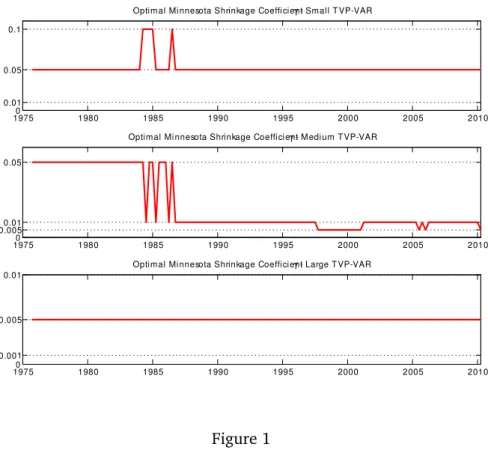
The main focus of this paper is on forecasting, but it is useful to briefly present some empirical evidence on other aspects of our approach. Figure 1 plots the selected value ofγ, the shrinkage parameter in the Minnesota prior, at each point in time for TVP-VARs of different dimension. Note that, as expected, we are finding that the necessary degree of shrinkage increases as the dimension of the TVP-VAR increases.

Figure 2 plots the optimal value of λselected by DMS at each point in time for the small, medium and large TVP-VARs. Note that, although there is some variation over time, the optimal value forλtends to be one, indicating relatively little change in the VAR coefficients. This holds true for TVP-VARs of all dimensions.

19750 1980 1985 1990 1995 2000 2005 2010

0.01 0.05 0.1

Optimal Mi nnesota Shrinkage Coeffi ci entγ - Sm all T VP-VAR

19750 1980 1985 1990 1995 2000 2005 2010

0.0050.01 0.05

Optimal Mi nnesota Shrinkage Coeffi ci entγ - M edi um T VP-VAR

19750 1980 1985 1990 1995 2000 2005 2010

0.001 0.005 0.01

Optimal Mi nnesota Shrinkage Coeffi ci entγ - Large T VP-VAR

(17)

1975 1980 1985 1990 1995 2000 2005 2010 0.97

0.98 0.99 1

Optimalλ - Sm all T VP-VAR

1975 1980 1985 1990 1995 2000 2005 2010

0.95 1

Optimalλ - M edi um T VP-VAR

1975 1980 1985 1990 1995 2000 2005 2010 0.95 0.97 0.98 0.99 1

Optimalλ - Large T VP-VAR

Figure 2

Figure 3 plots the time-varying probabilities associated with the TVP-VAR of each dimen-sion. DMS forecasts using the TVP-VAR of dimension with highest probability. It can be seen that this leads to a great deal of switching between TVP-VARs of different dimension. For un-stable periods (e.g. between, approximately, 1975-1985 or after 2008), DMS uses medium or large TVP-VARs to produce forecasts. In more stable times, the small TVP-VAR is often used (al-though there are some exceptions to this pattern, particularly in the 1990s when the medium TVP-VAR is chosen).

(18)

19600 1965 1970 1975 1980 1985 1990 1995 2000 2005 2010 0.1 0.2 0.3 0.4 0.5 0.6 0.7 0.8

T im e-varying probabili ties of smal l/medium /large VARs

small VAR medi um VAR large VAR

Figure 3

3.4 Forecast Comparison

We present iterated forecasts for horizons of up to two years (h = 1, ..,8) with a forecast evaluation period of 1975Q1 through 2010Q2. The use of iterated forecasts does increase the computational burden since predictive simulation is required (i.e. when h > 1 an analytical formula for the predictive density does not exist). We do predictive simulation in two different ways. The first (simpler) way uses the VAR coefficients which hold at time T to forecast variables at timeT +h. This assumes no VAR coefficient change between T andT +h. The second way, labelledβ_T+h∼RW in the tables, does allow for coefficient change out-of-sample and simulates from the random walk state equation (1) to produce draws ofβ_T+h. Both ways provide us withβ_T+h and we simulate draws ofyτ+h conditional onβT+hto approximate the

(19)

predictive density.7

The alternative would be to use direct forecasting, but recent papers such as Marcellino, Stock and Watson (2006) tend to find that iterated forecasts are better. Direct forecasting would also require re-estimating the model for different choices ofhand would not necessarily remove the need for predictive simulation since the researcher may wish to simulateβ_T+hfrom (1) whenh >1.

As measures of forecast performance, we use mean squared forecast errors (MSFEs) and predictive likelihoods. The latter are popular with many Bayesians since they evaluate the forecast performance of the entire predictive density (as opposed to merely the point forecast). Thus, Tables 1 through 3 (4 through 6) present MSFEs (sums of log predictive likelihoods) for each of our three variables of interest separately.8 _{We do both DMS and}

TVP-VAR-DMA and normalize our table relative to the latter. Thus, MSFEs and sums of log predictive likelihoods are presented relative to the TVP-VAR-DMA approach which simulatesβ_T+h from the random walk state equation. To be precise, the numbers in Tables 1 to 3 are ratios of the MSFE for a particular model divided by the MSFE of TVP-VAR-DMA and those in Tables 4 through 6 are the sums of log predictive likelihoods for a specific model minus the sum of log predictive likelihoods for TVP-VAR-DMA.

7_{For longer-term forecasting, this has the slight drawback that our approach is based on the model updating}

equation (see equation 8) which uses one-step ahead predictive likelihoods (which may not be ideal when fore-castingh >1periods ahead).

8_{For the reader interested in the joint log predictive likelihood for all three variables of interest, we note that}

this tends to be very similar to the sum of the three individual log predictive likelihoods and, thus, is not presented for the sake of brevity.

(20)

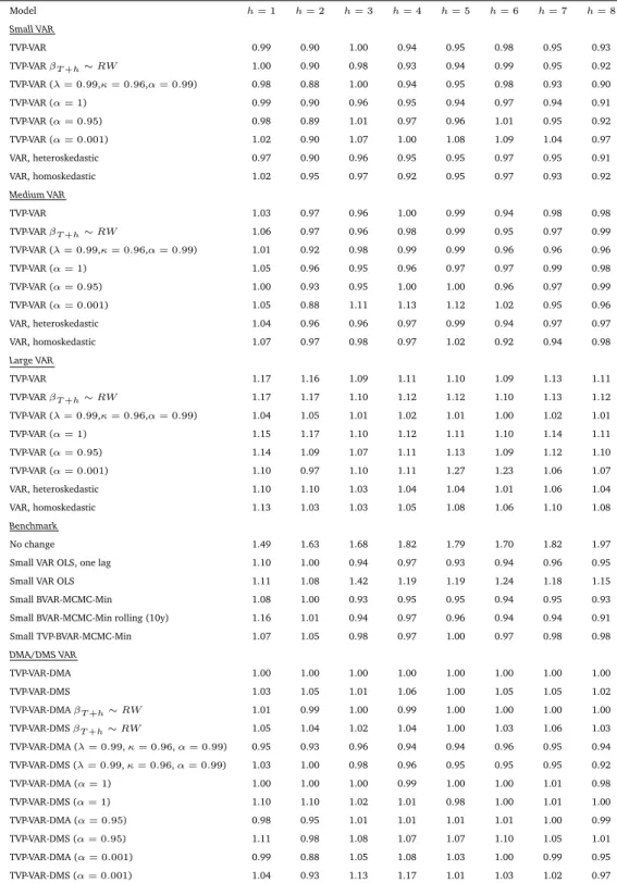
Table 1: MSFE relative to TVP-VAR-DMA, GDP Model h= 1 h= 2 h= 3 h= 4 h= 5 h= 6 h= 7 h= 8 Small VAR TVP-VAR 0.99 0.90 1.00 0.94 0.95 0.98 0.95 0.93 TVP-VARβT+h∼RW 1.00 0.90 0.98 0.93 0.94 0.99 0.95 0.92 TVP-VAR (λ= 0.99_,κ= 0.96_,α= 0.99₎ _0.98 _0.88 _1.00 _0.94 _0.95 _0.98 _0.93 _0.90 TVP-VAR (α= 1₎ _0.99 _0.90 _0.96 _0.95 _0.94 _0.97 _0.94 _0.91 TVP-VAR (α= 0.95₎ _0.98 _0.89 _1.01 _0.97 _0.96 _1.01 _0.95 _0.92 TVP-VAR (α= 0.001₎ _1.02 _0.90 _1.07 _1.00 _1.08 _1.09 _1.04 _0.97 VAR, heteroskedastic 0.97 0.90 0.96 0.95 0.95 0.97 0.95 0.91 VAR, homoskedastic 1.02 0.95 0.97 0.92 0.95 0.97 0.93 0.92 Medium VAR TVP-VAR 1.03 0.97 0.96 1.00 0.99 0.94 0.98 0.98 TVP-VARβT+h∼RW 1.06 0.97 0.96 0.98 0.99 0.95 0.97 0.99 TVP-VAR (λ= 0.99,κ= 0.96,α= 0.99) 1.01 0.92 0.98 0.99 0.99 0.96 0.96 0.96 TVP-VAR (α= 1) 1.05 0.96 0.95 0.96 0.97 0.97 0.99 0.98 TVP-VAR (α= 0.95) 1.00 0.93 0.95 1.00 1.00 0.96 0.97 0.99 TVP-VAR (α= 0.001₎ _1.05 _0.88 _1.11 _1.13 _1.12 _1.02 _0.95 _0.96 VAR, heteroskedastic 1.04 0.96 0.96 0.97 0.99 0.94 0.97 0.97 VAR, homoskedastic 1.07 0.97 0.98 0.97 1.02 0.92 0.94 0.98 Large VAR TVP-VAR 1.17 1.16 1.09 1.11 1.10 1.09 1.13 1.11 TVP-VARβT+h∼RW 1.17 1.17 1.10 1.12 1.12 1.10 1.13 1.12 TVP-VAR (λ= 0.99,κ= 0.96,α= 0.99) 1.04 1.05 1.01 1.02 1.01 1.00 1.02 1.01 TVP-VAR (α= 1) 1.15 1.17 1.10 1.12 1.11 1.10 1.14 1.11 TVP-VAR (α= 0.95) 1.14 1.09 1.07 1.11 1.13 1.09 1.12 1.10 TVP-VAR (α= 0.001) 1.10 0.97 1.10 1.11 1.27 1.23 1.06 1.07 VAR, heteroskedastic 1.10 1.10 1.03 1.04 1.04 1.01 1.06 1.04 VAR, homoskedastic 1.13 1.03 1.03 1.05 1.08 1.06 1.10 1.08 Benchmark No change 1.49 1.63 1.68 1.82 1.79 1.70 1.82 1.97

Small VAR OLS, one lag 1.10 1.00 0.94 0.97 0.93 0.94 0.96 0.95

Small VAR OLS 1.11 1.08 1.42 1.19 1.19 1.24 1.18 1.15

Small BVAR-MCMC-Min 1.08 1.00 0.93 0.95 0.95 0.94 0.95 0.93

Small BVAR-MCMC-Min rolling (10y) 1.16 1.01 0.94 0.97 0.96 0.94 0.94 0.91

Small TVP-BVAR-MCMC-Min 1.07 1.05 0.98 0.97 1.00 0.97 0.98 0.98 DMA/DMS VAR TVP-VAR-DMA 1.00 1.00 1.00 1.00 1.00 1.00 1.00 1.00 TVP-VAR-DMS 1.03 1.05 1.01 1.06 1.00 1.05 1.05 1.02 TVP-VAR-DMAβT+h∼RW 1.01 0.99 1.00 0.99 1.00 1.00 1.00 1.00 TVP-VAR-DMSβT+h∼RW 1.05 1.04 1.02 1.04 1.00 1.03 1.06 1.03 TVP-VAR-DMA (λ= 0.99,κ= 0.96,α= 0.99) 0.95 0.93 0.96 0.94 0.94 0.96 0.95 0.94 TVP-VAR-DMS (λ= 0.99,κ= 0.96,α= 0.99) 1.03 1.00 0.98 0.96 0.95 0.95 0.95 0.92 TVP-VAR-DMA (α= 1) 1.00 1.00 1.00 0.99 1.00 1.00 1.01 0.98 TVP-VAR-DMS (α= 1₎ _1.10 _1.10 _1.02 _1.01 _0.98 _1.00 _1.01 _1.00 TVP-VAR-DMA (α= 0.95₎ _0.98 _0.95 _1.01 _1.01 _1.01 _1.01 _1.00 _0.99 TVP-VAR-DMS (α= 0.95₎ _1.11 _0.98 _1.08 _1.07 _1.07 _1.10 _1.05 _1.01 TVP-VAR-DMA (α= 0.001₎ _0.99 _0.88 _1.05 _1.08 _1.03 _1.00 _0.99 _0.95 TVP-VAR-DMS (α= 0.001₎ _1.04 _0.93 _1.13 _1.17 _1.01 _1.03 _1.02 _0.97

(21)

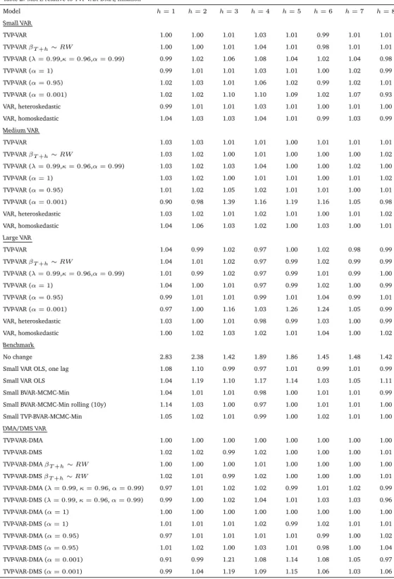
Table 2: MSFE relative to TVP-VAR-DMA, Inflation Model h= 1 h= 2 h= 3 h= 4 h= 5 h= 6 h= 7 h= 8 Small VAR TVP-VAR 1.00 1.00 1.01 1.03 1.01 0.99 1.01 1.01 TVP-VARβT+h∼RW 1.00 1.00 1.01 1.04 1.01 0.98 1.01 1.01 TVP-VAR (λ= 0.99_,κ= 0.96_,α= 0.99₎ _0.99 _1.02 _1.06 _1.08 _1.04 _1.02 _1.04 _0.98 TVP-VAR (α= 1₎ _0.99 _1.01 _1.01 _1.03 _1.01 _1.00 _1.02 _0.99 TVP-VAR (α= 0.95₎ _1.02 _1.03 _1.01 _1.06 _1.02 _0.99 _1.02 _1.01 TVP-VAR (α= 0.001₎ _1.02 _1.02 _1.10 _1.10 _1.09 _1.02 _1.07 _0.93 VAR, heteroskedastic 0.99 1.01 1.01 1.03 1.01 1.00 1.01 1.00 VAR, homoskedastic 1.04 1.03 1.03 1.04 1.01 0.99 1.03 0.99 Medium VAR TVP-VAR 1.03 1.03 1.01 1.01 1.00 1.01 1.01 1.01 TVP-VARβT+h∼RW 1.03 1.02 1.00 1.01 1.00 1.00 1.00 1.02 TVP-VAR (λ= 0.99,κ= 0.96,α= 0.99) 1.03 1.02 1.03 1.04 1.00 1.00 1.02 1.00 TVP-VAR (α= 1) 1.03 1.02 1.00 1.01 1.01 1.00 1.01 1.02 TVP-VAR (α= 0.95) 1.01 1.02 1.05 1.02 1.01 1.01 1.00 1.01 TVP-VAR (α= 0.001₎ _0.90 _0.98 _1.39 _1.16 _1.19 _1.16 _1.05 _0.98 VAR, heteroskedastic 1.03 1.02 1.01 1.02 1.01 1.00 1.01 1.02 VAR, homoskedastic 1.04 1.06 1.03 1.02 1.00 1.03 1.00 1.01 Large VAR TVP-VAR 1.04 0.99 1.02 0.97 1.00 1.02 0.98 0.99 TVP-VARβT+h∼RW 1.04 1.01 1.02 0.97 0.99 1.02 0.99 0.99 TVP-VAR (λ= 0.99,κ= 0.96,α= 0.99) 1.01 0.99 1.02 0.97 0.99 1.01 0.99 1.00 TVP-VAR (α= 1) 1.04 1.00 1.01 0.97 0.99 1.02 1.00 0.99 TVP-VAR (α= 0.95) 0.99 1.01 1.01 0.99 1.01 1.04 0.99 1.01 TVP-VAR (α= 0.001) 0.97 1.00 1.16 1.03 1.26 1.24 1.05 0.99 VAR, heteroskedastic 1.03 1.00 1.01 0.98 0.99 1.03 1.00 0.99 VAR, homoskedastic 1.00 1.02 1.03 1.02 1.01 1.04 1.00 1.02 Benchmark No change 2.83 2.38 1.42 1.89 1.86 1.45 1.48 1.42

Small VAR OLS 1.04 1.19 1.10 1.17 1.14 1.03 1.05 1.11

(22)

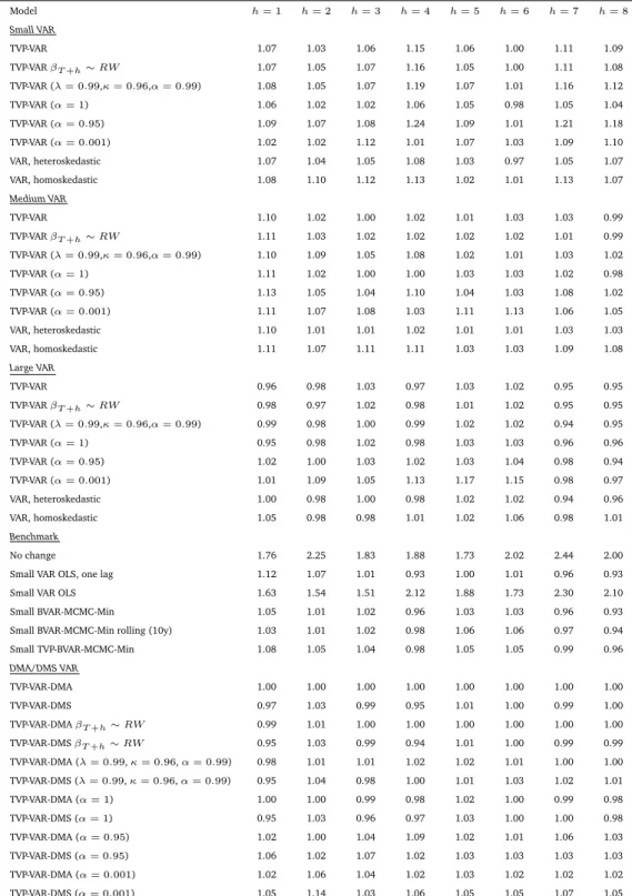
Table 3: MSFE relative to TVP-VAR-DMA, Interest Rate Model h= 1 h= 2 h= 3 h= 4 h= 5 h= 6 h= 7 h= 8 Small VAR TVP-VAR 1.07 1.03 1.06 1.15 1.06 1.00 1.11 1.09 TVP-VARβT+h∼RW 1.07 1.05 1.07 1.16 1.05 1.00 1.11 1.08 TVP-VAR (λ= 0.99_,κ= 0.96_,α= 0.99₎ _1.08 _1.05 _1.07 _1.19 _1.07 _1.01 _1.16 _1.12 TVP-VAR (α= 1₎ _1.06 _1.02 _1.02 _1.06 _1.05 _0.98 _1.05 _1.04 TVP-VAR (α= 0.95₎ _1.09 _1.07 _1.08 _1.24 _1.09 _1.01 _1.21 _1.18 TVP-VAR (α= 0.001₎ _1.02 _1.02 _1.12 _1.01 _1.07 _1.03 _1.09 _1.10 VAR, heteroskedastic 1.07 1.04 1.05 1.08 1.03 0.97 1.05 1.07 VAR, homoskedastic 1.08 1.10 1.12 1.13 1.02 1.01 1.13 1.07 Medium VAR TVP-VAR 1.10 1.02 1.00 1.02 1.01 1.03 1.03 0.99 TVP-VARβT+h∼RW 1.11 1.03 1.02 1.02 1.02 1.02 1.01 0.99 TVP-VAR (λ= 0.99,κ= 0.96,α= 0.99) 1.10 1.09 1.05 1.08 1.02 1.01 1.03 1.02 TVP-VAR (α= 1) 1.11 1.02 1.00 1.00 1.03 1.03 1.02 0.98 TVP-VAR (α= 0.95) 1.13 1.05 1.04 1.10 1.04 1.03 1.08 1.02 TVP-VAR (α= 0.001₎ _1.11 _1.07 _1.08 _1.03 _1.11 _1.13 _1.06 _1.05 VAR, heteroskedastic 1.10 1.01 1.01 1.02 1.01 1.01 1.03 1.03 VAR, homoskedastic 1.11 1.07 1.11 1.11 1.03 1.03 1.09 1.08 Large VAR TVP-VAR 0.96 0.98 1.03 0.97 1.03 1.02 0.95 0.95 TVP-VARβT+h∼RW 0.98 0.97 1.02 0.98 1.01 1.02 0.95 0.95 TVP-VAR (λ= 0.99,κ= 0.96,α= 0.99) 0.99 0.98 1.00 0.99 1.02 1.02 0.94 0.95 TVP-VAR (α= 1) 0.95 0.98 1.02 0.98 1.03 1.03 0.96 0.96 TVP-VAR (α= 0.95) 1.02 1.00 1.03 1.02 1.03 1.04 0.98 0.94 TVP-VAR (α= 0.001) 1.01 1.09 1.05 1.13 1.17 1.15 0.98 0.97 VAR, heteroskedastic 1.00 0.98 1.00 0.98 1.02 1.02 0.94 0.96 VAR, homoskedastic 1.05 0.98 0.98 1.01 1.02 1.06 0.98 1.01 Benchmark No change 1.76 2.25 1.83 1.88 1.73 2.02 2.44 2.00

Small VAR OLS 1.63 1.54 1.51 2.12 1.88 1.73 2.30 2.10

(23)

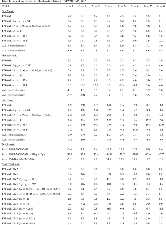
Table 4: Sum of log Predictive Likelihoods relative to TVP-VAR-DMA, GDP Model h= 1 h= 2 h= 3 h= 4 h= 5 h= 6 h= 7 h= 8 Small VAR TVP-VAR 7.1 6.3 4.2 4.6 2.5 4.3 4.5 5.1 TVP-VARβT+h∼RW 6.2 6.5 4.3 3.7 4.2 6.2 5.5 5.1 TVP-VAR (λ= 0.99_,κ= 0.96_,α= 0.99₎ _4.7 _8.9 _6.9 _9.1 _8.6 _9.0 _9.8 _8.4 TVP-VAR (α= 1₎ _6.0 _7.4 _5.1 _5.5 _5.4 _4.5 _6.5 _5.3 TVP-VAR (α= 0.95₎ _5.2 _7.3 _3.4 _3.3 _3.6 _4.3 _5.6 _4.6 TVP-VAR (α= 0.001₎ _8.6 _11.9 _7.8 _8.6 _2.4 _5.0 _7.8 _12.0 VAR, heteroskedastic 6.0 6.4 6.4 7.5 5.9 6.3 7.1 7.0 VAR, homoskedastic -6.0 1.3 2.6 6.7 6.6 5.7 5.6 4.5 Medium VAR TVP-VAR 2.6 5.0 5.7 3.1 5.2 4.5 3.7 2.4 TVP-VARβT+h∼RW 0.9 4.8 6.0 5.6 4.5 4.5 4.3 4.0 TVP-VAR (λ= 0.99,κ= 0.96,α= 0.99) 0.4 5.2 6.5 6.7 6.5 7.6 6.2 5.0 TVP-VAR (α= 1) 1.7 5.2 8.0 7.3 6.5 5.6 3.0 3.1 TVP-VAR (α= 0.95) 4.4 8.5 7.9 6.6 4.2 4.6 3.6 2.5 TVP-VAR (α= 0.001₎ _5.5 _11.3 _12.8 _5.6 _-3.5 _-4.3 _3.4 _4.6 VAR, heteroskedastic -0.1 4.6 5.8 6.2 4.1 6.1 3.7 3.8 VAR, homoskedastic -7.7 -2.0 2.2 5.1 3.1 5.6 3.5 1.7 Large VAR TVP-VAR -6.0 -9.8 -6.7 -6.3 -6.5 -7.2 -8.7 -8.4 TVP-VARβT+h∼RW -6.3 -8.6 -8.2 -4.9 -6.2 -5.7 -8.1 -8.8 TVP-VAR (λ= 0.99,κ= 0.96,α= 0.99) -3.2 -3.3 -2.3 -3.3 -4.4 -3.4 -6.9 -5.8 TVP-VAR (α= 1) -6.2 -8.1 -8.0 -6.0 -6.0 -6.5 -10.8 -9.2 TVP-VAR (α= 0.95) -2.8 -5.6 -6.5 -7.9 -8.2 -9.4 -10.8 -11.0 TVP-VAR (α= 0.001) -1.2 3.4 1.6 -1.5 -9.3 -14.8 -9.8 -8.8 VAR, heteroskedastic -2.0 -3.4 0.2 1.0 0.4 1.7 -1.6 -1.6 VAR, homoskedastic -14.1 -9.9 -5.1 -3.5 -4.8 -5.7 -8.5 -9.5 Benchmark Small BVAR-MCMC-Min -3.4 1.7 8.4 10.7 10.3 10.3 9.0 8.4

Small BVAR-MCMC-Min rolling (10y) -38.9 -37.8 -36.4 -34.8 -38.7 -39.8 -43.6 -42.7

Small TVP-BVAR-MCMC-Min -2.2 3.5 8.6 14.2 12.8 12.8 12.7 10.2 DMA/DMS VAR TVP-VAR-DMA 0.0 0.0 0.0 0.0 0.0 0.0 0.0 0.0 TVP-VAR-DMS -1.6 -2.6 -1.1 -4.3 -2.5 -2.2 0.6 0.5 TVP-VAR-DMAβT+h∼RW 0.7 0.3 0.8 1.3 0.0 0.9 -0.4 -0.3 TVP-VAR-DMSβT+h∼RW -1.0 -2.6 -0.5 -2.3 -1.5 -0.1 -1.2 -0.6 TVP-VAR-DMA (λ= 0.99,κ= 0.96,α= 0.99) 3.1 6.1 6.4 7.2 5.8 7.6 6.1 5.5 TVP-VAR-DMS (λ= 0.99,κ= 0.96,α= 0.99) 2.7 4.5 5.2 7.8 7.2 10.0 7.7 8.4 TVP-VAR-DMA (α= 1) 1.8 0.6 0.6 1.2 0.2 1.8 0.3 0.5 TVP-VAR-DMS (α= 1) 0.2 -4.2 -2.8 -1.6 0.6 0.8 0.0 0.0 TVP-VAR-DMA (α= 0.95) 2.0 3.3 0.5 -0.5 -0.6 0.1 -0.7 -0.3 TVP-VAR-DMS (α= 0.95) 1.5 5.4 -0.2 -2.1 -1.7 -0.6 1.9 2.9 TVP-VAR-DMA (α= 0.001₎ _3.9 _8.3 _5.8 _4.1 _-3.5 _-5.4 _1.0 _2.7 TVP-VAR-DMS (α= 0.001₎ _4.4 _9.0 _3.9 _3.3 _-5.8 _-4.2 _0.5 _1.5

(24)

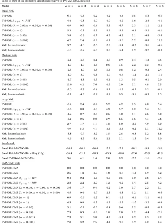
Table 5: Sum of log Predictive Likelihoods relative to TVP-VAR-DMA, Inflation Model h= 1 h= 2 h= 3 h= 4 h= 5 h= 6 h= 7 h= 8 Small VAR TVP-VAR 6.1 -0.6 -0.2 -4.2 -4.8 0.5 -5.4 -6.5 TVP-VARβT+h∼RW 4.4 -0.8 -1.0 -4.0 -4.2 1.6 -2.4 -4.1 TVP-VAR (λ= 0.99_,κ= 0.96_,α= 0.99₎ _4.9 _0.5 _-0.4 _-5.5 _-6.7 _2.3 _-1.1 _-2.2 TVP-VAR (α= 1₎ _5.3 _-0.8 _-2.5 _-3.9 _-5.3 _-0.3 _-5.2 _-4.1 TVP-VAR (α= 0.95₎ _3.8 _-0.8 _-1.7 _-4.3 _-4.8 _2.1 _-4.8 _-3.8 TVP-VAR (α= 0.001₎ _4.2 _2.4 _-1.8 _-6.1 _-5.6 _5.2 _-0.8 _11.8 VAR, heteroskedastic 3.7 -1.3 -2.3 -7.5 -5.4 -0.3 -3.6 -4.6 VAR, homoskedastic -6.3 -3.2 -5.5 -9.0 -5.4 1.9 -3.7 -0.3 Medium VAR TVP-VAR -2.1 -2.6 -0.1 -1.7 0.9 0.4 -1.3 0.5 TVP-VARβT+h∼RW -1.7 -1.7 -1.6 0.6 1.5 2.2 0.3 -0.5 TVP-VAR (λ= 0.99,κ= 0.96,α= 0.99) -2.5 -1.0 -1.8 -5.3 0.8 1.2 -0.3 2.4 TVP-VAR (α= 1) -1.0 -3.0 -0.3 -1.9 -0.4 -1.2 -2.1 -1.1 TVP-VAR (α= 0.95) -1.7 -1.8 -1.6 -0.1 1.3 0.5 -0.1 2.0 TVP-VAR (α= 0.001₎ _11.0 _4.2 _7.6 _-0.6 _2.0 _3.1 _4.8 _7.5 VAR, heteroskedastic -3.0 -2.8 -0.4 -3.8 -1.5 -0.2 0.2 -0.1 VAR, homoskedastic -3.1 -4.3 -2.9 -3.9 0.5 -3.1 -0.5 1.3 Large VAR TVP-VAR -3.2 2.4 -0.7 5.2 4.2 1.5 4.0 5.4 TVP-VARβT+h∼RW -3.6 0.8 -1.5 4.3 5.7 0.2 5.4 6.1 TVP-VAR (λ= 0.99,κ= 0.96,α= 0.99) -1.2 0.7 -2.6 2.6 4.0 1.1 2.6 4.0 TVP-VAR (α= 1) -3.1 0.6 0.0 3.9 6.5 1.6 4.1 7.6 TVP-VAR (α= 0.95) 2.7 1.7 1.1 1.8 5.0 -3.5 4.9 5.0 TVP-VAR (α= 0.001) 4.9 5.3 4.1 -3.5 -3.8 -0.2 1.1 11.0 VAR, heteroskedastic -3.8 -0.7 -3.2 1.5 2.8 -0.5 3.2 5.8 VAR, homoskedastic -4.6 -1.3 -5.4 -2.1 1.1 -1.5 0.4 1.0 Benchmark Small BVAR-MCMC-Min -16.8 -10.1 -10.8 -7.2 -7.9 -10.1 -9.9 -3.0

Small TVP-BVAR-MCMC-Min 3.6 4.1 1.4 2.0 0.9 -2.3 -1.6 -2.6 DMA/DMS VAR TVP-VAR-DMA 0.0 0.0 0.0 0.0 0.0 0.0 0.0 0.0 TVP-VAR-DMS 2.5 1.8 -1.0 1.0 -0.7 -1.3 1.9 4.2 TVP-VAR-DMAβT+h∼RW 0.4 0.2 -1.5 -0.5 0.5 1.0 0.6 1.4 TVP-VAR-DMSβT+h∼RW 2.8 2.2 -2.0 1.2 -0.2 1.4 2.5 4.2 TVP-VAR-DMA (λ= 0.99,κ= 0.96,α= 0.99) 3.6 1.7 0.4 -0.2 1.0 3.7 2.2 3.1 TVP-VAR-DMS (λ= 0.99,κ= 0.96,α= 0.99) 4.5 0.4 -1.9 -2.3 -4.8 1.2 1.1 -0.6 TVP-VAR-DMA (α= 1) 0.9 -0.9 -1.2 0.1 -1.2 -0.1 -1.1 -0.2 TVP-VAR-DMS (α= 1) 4.5 0.8 -1.2 -1.5 -2.3 -1.6 -3.2 -0.4 TVP-VAR-DMA (α= 0.95) 3.1 -0.2 -0.6 -0.4 0.4 1.2 -0.8 -0.5 TVP-VAR-DMS (α= 0.95) 7.9 0.3 -1.8 1.8 2.0 2.2 -4.4 -2.1 TVP-VAR-DMA (α= 0.001₎ _7.3 _3.1 _3.8 _-4.7 _-5.1 _2.9 _2.3 _9.2 TVP-VAR-DMS (α= 0.001₎ _7.8 _3.2 _7.5 _-4.1 _-9.3 _3.9 _4.2 _1.4

(25)

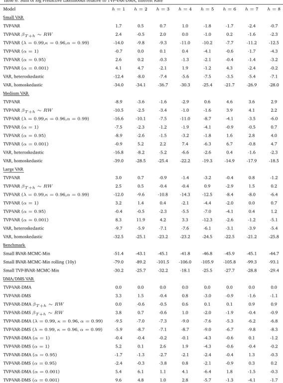
Table 6: Sum of log Predictive Likelihoods relative to TVP-VAR-DMA, Interest Rate Model h= 1 h= 2 h= 3 h= 4 h= 5 h= 6 h= 7 h= 8 Small VAR TVP-VAR 1.7 0.5 0.7 1.0 -1.8 -1.7 -2.4 -0.7 TVP-VARβT+h∼RW 2.4 -0.5 2.0 0.0 -1.0 0.2 -1.6 -2.3 TVP-VAR (λ= 0.99_,κ= 0.96_,α= 0.99₎ _-14.0 _-9.8 _-9.3 _-11.0 _-10.2 _-7.7 _-11.2 _-12.5 TVP-VAR (α= 1₎ _-0.7 _0.0 _0.1 _0.4 _-4.1 _-0.6 _-1.7 _-4.3 TVP-VAR (α= 0.95₎ _2.6 _0.2 _-0.3 _-1.3 _-2.1 _-0.4 _-1.4 _-3.2 TVP-VAR (α= 0.001₎ _4.1 _4.7 _-2.1 _1.9 _-1.2 _4.3 _-2.4 _-0.2 VAR, heteroskedastic -12.4 -8.0 -7.4 -5.6 -7.5 -3.5 -5.4 -7.1 VAR, homoskedastic -34.0 -34.1 -36.7 -30.3 -25.4 -21.7 -26.9 -28.0 Medium VAR TVP-VAR -8.9 -3.6 -1.6 -2.9 0.6 4.6 3.6 2.9 TVP-VARβT+h∼RW -10.5 -2.5 -3.4 -1.0 -1.6 3.9 4.1 2.2 TVP-VAR (λ= 0.99,κ= 0.96,α= 0.99) -16.6 -10.1 -7.5 -11.0 -8.7 -4.1 -3.5 -6.0 TVP-VAR (α= 1) -7.5 -2.3 -1.2 -1.9 -4.1 -0.9 -0.5 0.7 TVP-VAR (α= 0.95) -8.9 -2.6 -1.5 -3.2 -1.8 1.6 2.8 4.0 TVP-VAR (α= 0.001₎ _-0.9 _5.2 _2.2 _7.4 _-6.3 _6.7 _-0.8 _4.7 VAR, heteroskedastic -16.8 -8.2 -5.2 -6.6 -2.6 0.4 -1.6 -2.3 VAR, homoskedastic -39.0 -28.5 -25.4 -22.2 -19.3 -14.9 -17.9 -18.5 Large VAR TVP-VAR 3.0 0.7 -0.9 -1.4 -3.2 -0.4 0.8 -1.2 TVP-VARβT+h∼RW 2.5 0.5 -0.4 -0.4 0.9 -2.9 1.5 0.2 TVP-VAR (λ= 0.99,κ= 0.96,α= 0.99) -12.0 -9.6 -10.8 -14.3 -12.5 -8.4 -8.0 -6.4 TVP-VAR (α= 1) 3.2 1.4 0.4 -2.1 -4.4 -2.0 0.0 0.7 TVP-VAR (α= 0.95) -0.4 -0.5 -2.3 -5.5 -7.0 -4.1 0.4 1.2 TVP-VAR (α= 0.001) 8.3 11.9 4.2 3.3 -12.3 -2.6 -1.2 -5.1 VAR, heteroskedastic -9.7 -5.9 -7.1 -7.6 -6.1 -3.1 -3.9 -5.4 VAR, homoskedastic -32.5 -25.1 -23.2 -23.2 -24.5 -22.5 -21.2 -25.8 Benchmark Small BVAR-MCMC-Min -51.4 -43.1 -45.1 -41.8 -46.8 -45.9 -45.1 -44.7

Small TVP-BVAR-MCMC-Min -30.2 -25.7 -32.2 -18.1 -25.5 -27.7 -28.8 -29.4 DMA/DMS VAR TVP-VAR-DMA 0.0 0.0 0.0 0.0 0.0 0.0 0.0 0.0 TVP-VAR-DMS 3.3 1.5 -0.4 0.8 -3.0 -0.9 -1.6 -1.1 TVP-VAR-DMAβT+h∼RW 0.0 -0.6 -0.5 0.6 0.1 0.1 0.9 0.9 TVP-VAR-DMSβT+h∼RW 3.8 0.7 -0.6 1.0 -2.0 -1.9 -0.4 -0.9 TVP-VAR-DMA (λ= 0.99,κ= 0.96,α= 0.99) -9.5 -7.0 -7.3 -9.0 -7.6 -5.3 -6.2 -6.8 TVP-VAR-DMS (λ= 0.99,κ= 0.96,α= 0.99) -5.9 -8.7 -7.1 -8.7 -9.0 -6.7 -9.8 -8.3 TVP-VAR-DMA (α= 1) -0.4 -0.4 -0.2 -0.1 -4.3 -0.6 0.1 -1.2 TVP-VAR-DMS (α= 1) 5.2 0.1 2.6 1.9 -4.3 -0.6 -0.4 -0.2 TVP-VAR-DMA (α= 0.95) -1.7 -1.3 -2.7 -2.1 -2.4 -0.4 1.3 -0.3 TVP-VAR-DMS (α= 0.95) -2.4 -0.3 -3.8 0.8 -2.1 -0.9 0.3 0.2 TVP-VAR-DMA (α= 0.001₎ _5.4 _6.1 _1.1 _4.1 _-6.4 _1.8 _-1.5 _-0.3 TVP-VAR-DMS (α= 0.001₎ _9.6 _4.8 _1.0 _2.8 _-5.7 _-1.3 _-4.1 _-1.7

With three different variables, eight different forecast horizons and two different forecast metrics, there are many ways of comparing our forecasts. Virtually every model can be found to do well for some case. Broadly speaking, the MSFEs and log predictive likelihoods are telling the same story. Although our full TVP-VAR-DMS or DMA approaches are not always the best forecasting approaches, they are typically among the best and never forecast poorly. It is a

(26)

safe forecasting procedure which never goes too far wrong and automatically makes many of the necessary specification choices that a researcher faces. In contrast, other strategies such as always using a TVP-VAR of a fixed dimension can sometimes forecast very well, but also will sometimes forecast quite poorly.

With regards to the issue of TVP-VAR dimensionality, there is no single dimension that dom-inates. Sometimes the dimension-switching feature of our TVP-VAR-DMS approach leads to the best forecasting performance, but each of the small, medium and large TVP-VARs forecasts best for some forecast horizon for some variable. A general finding is that (with some exceptions), small TVP-VARs tend to be preferred for GDP, whereas large TVP-VARs are preferred for infla-tion. With interest rates there is conflicting evidence as to whether small, medium or large TVP-VARs are preferred which may explain why our full TVP-VAR-DMS approach tends to do particularly well for forecasting interest rates. Of course, any VAR or TVP-VAR model accom-modate forecasts of several variables at the same time, so it is not surprising that no single VAR dimension will be best for all variables. Our approach takes into account the total predictive likelihood of the three variables weighted equally. In practice, policy-makers might want to give more weight to one variable (such as inflation) rather than others. It would be simple to modify our algorithm to do this. Such a modification would enhance forecasts of inflation, probably at the cost of deteriorating forecasts of the other variables.9

The value of doing DMS is also clear in that approaches where this is done almost always beat benchmark approaches which do not. With the exception of GDP forecasting at long horizons, benchmark approaches involving small dimensional models such as the TVP-VAR of Primiceri (2005) which is labelled Small TVP-BVAR-MCMC-Min in the tables, the Minnesota prior VAR or the VAR estimated using OLS methods, forecast poorly relative to our TVP-VAR-DMS approach. For instance, if you look at Tables 1 through 6 and compare Small TVP-BVAR-MCMC-Min with the row labelled small TVP-VAR (which does DMS), you can see that the latter

9_{The finding that the forecast performance of individual variables changes with TVP-VAR dimension suggests}

that there might be additional benefit from combining an algorithm which selects explanatory variables with one which selects VAR dimension. For instance, such an approach could select a high dimensional VAR, but impose restrictions on explanatory variables such that the GDP equation only contains lags of a small number of variables, whereas the inflation equation contains lags of many more variables. We have used such algorithms in previous work (e.g. Korobilis, 2012 or Jochmann, Koop and Strachan, 2010), but they require the use of MCMC methods and, thus, are computationally daunting with large TVP-VARs.

(27)

always forecasts better than the former for h = 1. With some exceptions, this same patterns holds at longer forecast horizons.

Tables 1 through 6 also contain many variants of the TVP-VAR-DMS approach where α

is set to a particular value and where λ and κ are not estimated but rather set to standard values. With the exception of interest rates, the benefits of estimatingλandκare quite small. Indeed, for GDP forecasting, the case whereλandκare not estimated often leads to the best forecasting performance. With regards to the forgetting factor,α, we find results to be fairly robust over the commonly-used interval [0.95,1]. However, it is the α = 0.001 case which attaches equal probability to TVP-VARs of each dimension, that sometimes forecasts best. This finding is particularly interesting in light of recent work on prediction pools (e.g. Amisano and Geweke, 2012) which often find equally weighted pools of predictive densities to forecast well. Model averaging and model selection methods tend to produce similar forecasts. Overall TVP-VAR-DMA does forecast slightly better than TVP-VAR-DMS, but there are many exceptions to this pattern (particularly when using predictive likelihoods as a forecast metric).

With regards to predictive simulation, our results suggest that simulating β_T+h from the random walk state equation yields only modest forecast improvements over the simpler strat-egy of assuming no change in VAR coefficients over the horizon that the forecast is being made. The importance of allowing for heteroskedastic errors in getting the shape of the predictive density correct is clearly shown by the poor performance of homoskedastic models in Tables 4 through 6.

In summary, our results suggest that our methods provide an effective way of estimating even large TVP-VARs with heteroskedastic errors (which would be computationally infeasible using MCMC methods) and choosing prior shrinkage. In our application, it does seem that there is a great deal of uncertainty over TVP-VAR dimensionality. Any researcher who just worked with one dimension would do well in some cases, but badly in other cases. Hence, a method like ours which automatically selects the dimension in a time varying fashion is potentially of great use.

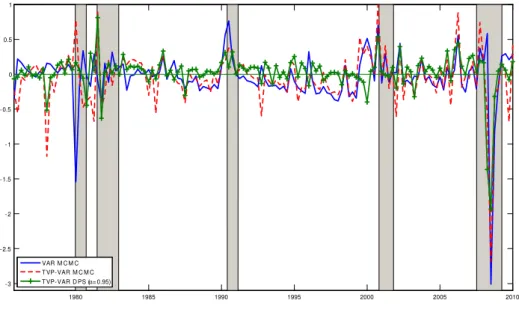
Figures 4 through 6 plot logs of one-step ahead predictive likelihoods (relative to the bench-mark TVP-VAR-DMA model) against time for our three variables of interest with NBER

(28)

reces-sion dates shaded. These figures allow for the comparison over time of our approach against several plausible alternatives. In particular, we compare the TVP-VAR-DMA approach to: i) the small Bayesian VAR with Minnesota prior; ii) the fully-specified Small TVP-BVAR-MCMC-Min model similar to that used by Primiceri (2005) and D’Agostino, Gambetti and Giannone (2011); and iii) the small TVP-VAR usingα = 0.99. Since all one-step ahead predictive likeli-hoods are relative to that of the benchmark TVP-VAR-DMA model, negative (positive) numbers indicate that our benchmark model is a better (worse) forecasting model for that time period. A pattern worth noting in these figures is that the small VAR model (with some exceptions) is forecasting relatively poorly during recessions (especially at their start). This holds partic-ularly true for inflation and GDP forecasting of the early 1980s recessions and the financial crisis.10 _{This pattern is also true for the Small TVP-BVAR-MCMC-Min model, but to a lesser}

extent. The fact that the TVP-VAR-DMS approach is forecasting particularly well during these recessions is consistent with patterns in Figure 3 where there is strong evidence for TVP-VAR dimension switching during these recessions.

However, it is not the case that TVP-VAR-DMS is always forecasting better in recessions, since for the recessions in the early 1990s and 2000s other methods are forecasting as well and sometimes better. And in the pre-Lehman part of the recent NBER-dated recession, TVP-VAR-DMS is also not forecasting particularly well.

Thus, when forecasting inflation and GDP, we are finding a superior performance of TVP-VAR-DMS in at least the major recessions. However, it is interesting to note that this finding does not completely carry over for interest rates. In the recessions of the early 1980s we are finding TVP-VAR-DMS to forecast interest rates better than other approaches. But this does not occur for the most recent recession. Instead, the superior average forecast performance of TVP-VAR-DMS for interest rates is obtained mostly during the long expansionary periods between the early 1990s and 2001 and between 2002 and 2007.

10_{Note that the NBER dates the recent recession as beginning in December 2007. However, the large deterioration}

(29)

1980 1985 1990 1995 2000 2005 2010 - 3 - 2.5 - 2 - 1.5 - 1 - 0.5 0 0.5 1 VAR M C M C T VP-VAR M C M C T VP-VAR D PS (α= 0.95)

Figure 4: Relative Log Predictive Likelihoods for GDP

1980 1985 1990 1995 2000 2005 2010 - 10 - 8 - 6 - 4 - 2 0 VAR M C M C T VP-VAR M C M C T VP-VAR D PS (α= 0.95)

(30)

1980 1985 1990 1995 2000 2005 2010 - 14 - 12 - 10 - 8 - 6 - 4 - 2 0 2 VAR M C M C T VP-VAR M C M C T VP-VAR -D PS (α= 0.95)

Figure 6: Relative Log Predictive Likelihoods for Interest Rates

4 Conclusions

In this paper, we have developed computationally feasible methods for forecasting with large TVP-VARs through the use of forgetting factors. We use forgetting factors in several ways. First, they allow for simple forecasting within a single TVP-VAR model. However, inspired by the literature on dynamic model averaging and selection (see Raftery et al, 2010), we also use forgetting factors so as to allow for fast and simple dynamic model selection. That is, we develop methods so that the forecasting model can change at every point in time.

DMS can be used with any type of model. We have found it useful to define our models in terms of their dimension, the priors that they use and the values of the decay and forgetting. These features allow us to estimate: i) the desired degree of evolution of VARs coefficients and volatilities, ii) the shrinkage parameter of the Minnesota prior and iii) the dimension of the TVP-VAR. Furthermore, all of these can change in a time-varying fashion and involve only a simple recursive updating scheme. In our empirical exercise, we have found our approach to

(31)

(32)

References

Amisano, G. and Geweke, J. (2012). “Prediction using several macroeconomic models,” man-uscript.

Banbura, M., Giannone, D. and Reichlin, L. (2010). “Large Bayesian vector auto regres-sions,”Journal of Applied Econometrics, 25, 71-92.

Brockwell, R. and Davis, P. (2009). Time series: Theory and methods(second edition). New York: Springer.

Canova, F. and Ciccarelli, M. (2009). “Estimating multicountry VAR models,”International

Economic Review, 50, 929-959.

Canova, F. and Forero, F. (2012). “Estimating overidentified, nonrecursive, time-varying coefficients structural VARs,” Universitat Pompeu Fabra, Economics Working Papers number 1321.

Carriero, A., Clark, T. and Marcellino, M. (2011). “Bayesian VARs: Specification choices and forecast accuracy,” Federal Reserve Bank of Cleveland, working paper 11-12.

Carriero, A., Clark, T. and Marcellino, M. (2012). “Common drifting volatility in large Bayesian VARs,” CEPR WP 8894.

Carriero, A., Kapetanios, G. and Marcellino, M. (2009). “Forecasting exchange rates with a large Bayesian VAR,”International Journal of Forecasting, 25, 400-417.

Chan, J., Koop, G., Leon-Gonzalez, R. and Strachan, R. (2012).“Time varying dimension models,”Journal of Business and Economic Statistics, forthcoming.

Cogley, T., Morozov, S. and Sargent, T. (2005). “Bayesian fan charts for U.K. inflation: Forecasting and sources of uncertainty in an evolving monetary system,”Journal of Economic

Dynamics and Control, 29, 1893-1925.

Cogley, T. and Sargent, T. (2001). “Evolving post World War II inflation dynamics,” NBER

Macroeconomics Annual, 16, 331-373.

Cogley, T. and Sargent, T. (2005). “Drifts and volatilities: Monetary policies and outcomes in the post WWII U.S.,”Review of Economic Dynamics, 8, 262-302.

(33)

structural change,”Journal of Applied Econometrics, doi: 10.1002/jae.1257.

Dangl, T. and Halling, M. (2012). “Predictive regressions with time varying coefficients,”

Journal of Financial Economics,forthcoming.

Ding, S. and Karlsson, S. (2012). “Model averaging and variable selection in VAR models,” manuscript.

Doan, T., Litterman, R. and Sims, C. (1984). “Forecasting and conditional projections using a realistic prior distribution”,Econometric Reviews,3, 1-100.

Fagin, S. (1964). “Recursive linear regression theory, optimal filter theory, and error analy-ses of optimal systems,”IEEE International Convention Record Part i, pages 216-240.

Fruhwirth-Schnatter, S., (2006). Finite Mixture and Markov Switching Models. New York: Springer.

Giannone, D., Lenza, M., Momferatou, D. and Onorante, L. (2010). “Short-term inflation projections: a Bayesian vector autoregressive approach,” ECARES working paper 2010-011, Universite Libre de Bruxelles.

Giannone, D., Lenza, M. and Primiceri, G. (2012). “Prior selection for vector autoregres-sions,”Centre for Economic Policy Research,working paper 8755.

Jazwinsky, A. (1970).Stochastic Processes and Filtering Theory. New York: Academic Press. Jochmann, J., Koop, G. and Strachan, R. (2010). “Bayesian forecasting using stochastic search variable selection in a VAR subject to breaks,”International Journal of Forecasting, 26, 326-347

Koop, G. (2011). “Forecasting with medium and large Bayesian VARs,” Journal of Applied

Econometrics, forthcoming.

Koop, G. and Korobilis, D. (2009). “Bayesian multivariate time series methods for empirical macroeconomics,”Foundations and Trends in Econometrics, 3, 267-358.

Koop, G. and Korobilis, D. (2012). “Forecasting inflation using dynamic model averaging,”

International Economic Review, 53, 867-886.

Koop, G., Leon-Gonzalez, R. and Strachan, R. (2009). “On the evolution of the monetary policy transmission mechanism,”Journal of Economic Dynamics and Control, 33, 997-1017.

(34)

Econometrics, doi: 10.1002/jae.1271.

Marcellino, M., Stock, J. and Watson, M. (2006). “A comparison of direct and iterated AR methods for forecasting macroeconomic series h-steps ahead,” Journal of Econometrics, 135, 499-526.

McCormick, T., Raftery, A. Madigan, D. and Burd, R. (2011). “Dynamic logistic regression and dynamic model averaging for binary classification,”Biometrics, forthcoming.

Primiceri, G. (2005). “Time varying structural vector autoregressions and monetary policy,”

Review of Economic Studies, 72, 821-852.

Raftery, A., Karny, M. and Ettler, P. (2010). “Online prediction under model uncertainty via dynamic model averaging: Application to a cold rolling mill,”Technometrics, 52, 52-66.

RiskMetrics (1996). Technical Document (Fourth Edition). Available at http://www. risk-metrics.com/system/files/private/td4e.pdf.

Stock, J. and Watson, M. (2008). “Forecasting in dynamic factor models subject to struc-tural instability,” in The Methodology and Practice of Econometrics, A Festschrift in Honour of

Professor David F. Hendry, edited by J. Castle and N. Shephard, Oxford: Oxford University

Press.

West, M. and Harrison, J. (1997). Bayesian Forecasting and Dynamic Models, second edition, New York: Springer.

(35)

A

Data Appendix

All series were downloaded from St. Louis’ FRED database and cover the quarters 1959:Q1 to 2010:Q2. Some series in the database were observed only on a monthly basis and quarterly values were computed by averaging the monthly values over the quarter. All variables are transformed to be approximately stationary following Stock and Watson (2008). In particular, ifzi,t is the original untransformed series, the transformation codes are (column Tcode below): 1 - no transformation (levels), xi,t = zi,t; 2 - first difference, xi,t = zi,t−zi,t−1; 3 - second difference, xi,t = zi,t−zi,t−2; 4 - logarithm, xi,t = logzi,t; 5 - first difference of logarithm,

xi,t = lnzi,t−lnzi,t−1; 6 - second difference of logarithm,xi,t = lnzi,t−lnzi,t−2.

Table A1: Series used in the Small TVP-VAR withn= 3

Series ID Tcode Description

GDPC96 5 Real Gross Domestic Product CPIAUCSL 6 Consumer Price Index: All Items FEDFUNDS 2 Effective Federal Funds Rate

Table A2: Additional series used in the Medium TVP-VAR withn= 7

Series ID Tcode Description

PMCP 1 NAPM Commodity Prices Index

BORROW 6 Borrowings of Depository Institutions from the Fed SP500 5 S&P 500 Index