differential item functioning in the
Rasch model
Carolin Strobl, Julia Kopf, Achim Zeileis
Working Papers in Economics and Statistics
2011-01
University of Innsbruck
The series is jointly edited and published by
-Department of Economics
-Department of Public Finance
-Department of Statistics Contact Address:
University of Innsbruck Department of Public Finance Universitaetsstrasse 15 A-6020 Innsbruck Austria Tel: + 43 512 507 7171 Fax: + 43 512 507 2970 e-mail: [email protected]
The most recent version of all working papers can be downloaded at
http://www.uibk.ac.at/fakultaeten/volkswirtschaft und statistik/forschung/wopec/ For a list of recent papers see the backpages of this paper.
functioning in the Rasch model
Carolin Strobl Ludwig-Maximilians-Universit¨at M¨unchen Julia Kopf Ludwig-Maximilians-Universit¨at M¨unchen Achim Zeileis Universit¨at Innsbruck AbstractDifferential item functioning (DIF) can lead to an unfair advantage or disadvantage for certain subgroups in educational and psychological testing. Therefore, a variety of statistical methods has been suggested for detecting DIF in the Rasch model. Most of these methods are designed for the comparison of pre-specified focal and reference groups, such as males and females. Latent class approaches, on the other hand, allow to detect previously unknown groups exhibiting DIF. However, this approach provides no straightforward interpretation of the groups with respect to person characteristics.
Here we propose a new method for DIF detection based on model-based recursive partitioning that can be considered as a compromise between those two extremes. With this approach it is possible to detect groups of subjects exhibiting DIF, which are not pre-specified, but result from combinations of observed covariates. These groups are directly interpretable and can thus help understand the psychological sources of DIF.
The statistical background and construction of the new method is first introduced by means of an instructive example, and then applied to data from a general knowledge quiz and a teaching evaluation.
Keywords: item response theory, IRT, Rasch model, differential item functioning, DIF, struc-tural change, multidimensionality.
1. Introduction
In educational and psychological testing, the term differential item functioning (DIF) ‘means that the probability of a correct response among equally able test takers is different for various racial, ethnic, gender [or other] subgroups. A given educational or psychological test consisting of many items with significant DIF may be unfair for certain subgroups, and it is important to identify these items, so that they can be improved or deleted from the test’ (Westers and Kelderman 1991).
A variety of statistical methods is available for detecting DIF in the Rasch model. While some of these methods are explicitly designed to detect DIF in individual items, such as the item-specific Wald test (Fischer and Molenaar 1995), others are global goodness-of-fit tests for the Rasch model that also respond to DIF, such as the likelihood ratio test (Andersen 1972). Most of these methods are based on the comparison of the item parameter estimates between two or more pre-specified groups of subjects, such as males and females as focal and reference groups. This class of model tests includes the widely used graphical test as well as
the most recent approaches based on a mixed model representation (Rijmen, Tuerlinckx, De Boeck, and Kuppens 2003;den Noortgate and De Boeck 2005).
The advantage of model tests for given groups is that, if DIF is detected, the results can be interpreted straightforwardly in terms of, e.g., wich items are easier or harder to solve for which group. This can give valuable hints at the psychological sources for the differential functioning of the items, and how it can be eliminated or avoided in future versions of the test, as also pointed out by Stout (2002): ‘. . . if reading-comprehension test items of paragraphs that discuss the physical sciences are discovered to display DIF against women, then the test specifications for future versions of such a reading comprehension test might exclude physical-science-based paragraphs’.
On the other hand, in all above mentioned approaches only those groups that are explicitly proposed by the researcher are tested for DIF. Variables typically proposed for testing include age, gender, ethnicity and language, depending on the objective of the assessment (cf., e.g.,
Gelin, Carleton, Smith, and Zumbo 2004; Perkins, Stump, Monahan, and McHorney 2006;
Woods, Oltmanns, and Turkheimer 2009; Pedraza, Graff-Radford, Smith, Ivnik, Willis, Pe-tersen, and Lucas 2009). However, if in later analyses a group difference is found in a variable that has not been explicitly tested for DIF, it cannot be ruled out that this effect is only an artefact due to unnoticed DIF.
At the other extreme, the latent class (or mixture) approach ofRost(1990) can be considered as the most stringent test for the Rasch model, because it tests for item parameter differences between all possible groups of subjects – regardless of person covariates. In this sense, the latent class approach is a very stringent model test, but it provides no straightforward inter-pretation of the groups. Therefore, often latent class approaches are used only as a first step in the analysis, where the second step is to attempt to describe the latent classes by person covariates for interpretability (see, e.g.,Cohen and Bolt 2005;Hancock and Samuelsen 2007;
de Meij, Kelderman, and van der Flier 2008, and the references therein).
Here, we propose a new statistical approach for detecting DIF in the Rasch model that can be considered a compromise between the two former approaches – testing only predefined (and hence easy to interpret) groups vs. testing all possible groups but loosing interpretability. The idea for the new method is to recursively test all groups that can be defined based on (interactions of) the available covariates, thus preserving interpretability, but still exploring a very wide set of potential sources of DIF.
In the next section, the rationale and technical details of the new method are first explained by means of a simple artificial example. Two applications to a general knowledge quiz and a teaching evaluation are presented in Section 3. The method is freely available as a software implementation in the add-on package psychotree (Zeileis, Strobl, Wickelmaier, and Kopf 2010) for the R system for statistical computing (R Development Core Team 2010).
2. A new method based on recursive partitioning
The new method for detecting groups of subjects with DIF is based on the technique of model-based recursive partitioning, that employs statistical tests for structural change adopted from econometrics. Model-based recursive partitioning is a semi-parametric approach. The aim is to detect differences in the parameters of a statistical model between groups of subjects defined by combinations of covariates.
Table 1: Summary statistics for the covariates of the instructive example (artificial data).
Variable Summary statistics
Gender male: 109 female: 91
xmin x0.25 xmed x¯ x0.75 xmax
Age 16 31 45 45.84 60 74
Motivation 1 2 3 3.38 5 6
Model-based recursive partitioning is related to the method of classification and regression trees (CART,Breiman, Friedman, Olshen, and Stone 1984; seeStrobl, Malley, and Tutz 2009
for a thorough introduction), where the covariate space is recursively partitioned to identify groups of subjects with different values of a categorical or continuous response variable. As an advancement of this approach, in model-based recursive partitioning it is the parameters of a parametric model – rather than the values of a single response variable – that vary between groups. Such parameters could be, e.g., intercept and slope parameters in a linear regression model or, as in our case, the item parameters of a Rasch model that may vary between groups of subjects.
This principle is now first illustrated by means of an artificial instructive example, before the technical details are addressed in the next sections: The data for the instructive example consist of the simulated responses of 200 subjects to 20 items, which can be considered, e.g., as questions in a proficiency test. In addition to the responses, the data set includes three covariates: gender, age, and a motivation score. The summary statistics for the latter are listed in Table1.
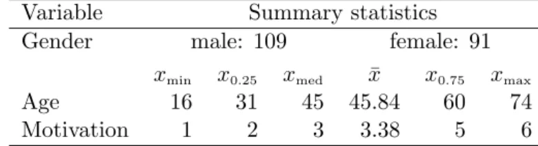
In order to test for DIF, the method assesses the item responses with respect to the three covariates: gender, age, and motivation. The result is presented in Figure 1 and will be termed a Rasch tree from here on. In each of the terminal nodes of the tree, the item parameter estimates for the 20 items are displayed (a high value indicates that the item is very difficult).
Following the tree from top to bottom, we find that different item parameters result for males and females, and within the group of males for those up to and over the age of 34. For example, the third item (highlighted by the large dot) is particularly hard for males up to the age of 34 (represented in node 3) as well as for females (represented in node 5), while the 14-th item (highlighted by the second large dot) is particulary easy only for the young males (represented in node 3). Note also that the variable motivation was not selected for splitting, i.e., there is no DIF with respect to motivation, but only with respect to gender and age. Generally speaking, the fact that we end up with more than one terminal node in Figure 1
means that the null hypothesis of one joint Rasch model for the entire sample must be rejected. In this sense, the proposed method is a test for DIF as well as an overall model test for the Rasch model. More importantly, however, we can directly see which groups are affected by DIF with respect to which items. This information can help identify the reasons for DIF and guide the decision how to proceed with the affected items.
The following consecutive steps are used to create the Rasch tree in Figure1:
1. Estimate the item parameters jointly for all subjects in the current sample, starting with the full sample.
gender p = 0.006 1 male female age p < 0.001 2 ≤34 >34 Node 3 (n = 35) ● ● ● ● ● ● ●● ● ● ● ● ● ● ● ● ● ● ● ● 1 20 −2.68 4.66 Node 4 (n = 74) ● ●●● ● ● ● ● ● ● ● ● ● ●● ● ● ● ● ● 1 20 −2.68 4.66 Node 5 (n = 91) ● ● ● ● ● ● ● ● ● ● ● ● ● ● ● ● ● ● ●● 1 20 −2.68 4.66
Figure 1: Rasch-tree for the instructive example (artificial data for illustration purposes), exhibiting DIF between males up to the age of 34, males over the age of 34 and females. In the terminal nodes, estimates of the item difficulty are displayed for each of the 20 items.
2. Assess the stability of the item parameters with respect to each available covariate. 3. If there is significant instability, split the sample along the covariate with the strongest
instability and in the cutpoint leading to the highest improvement of the model fit. 4. Repeat steps 1–3 recursively in the resulting subsamples until there are no more
signif-icant instabilities (or the subsample is too small). These steps are now explained in more detail.
2.1. Estimating the item parameters
We use the common conditional maximum likelihood approach for estimating the item param-eters (but the method can also be adapted to, e.g., marginal maximum likelihood estimation). Letθi,i= 1, . . . , n, denote the person parameters, βj,j= 1, . . . , m, denote the item
param-eters anduij denote the response of subject ito itemj. Since under the Rasch model
P(Uij =uij|θi, βj) =
euij·(θi−βj) 1 +eθi−βj
the person raw-scores ri form sufficient statistics for the person parameters, the item
pa-rameters can be estimated by means of iterative procedures from the conditional likelihood
Lc(β|r1, . . . , rn) = n Y i=1 Lc(β|ri) = n Y i=1 e−Pmj=1uij·βj γri(β) , (1)
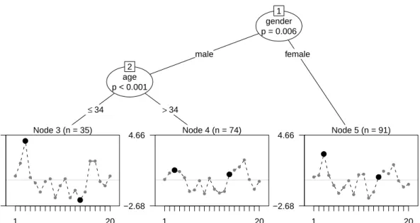
t y 2004 2006 2008 2010 2012 0.02 0.04 0.06 0.08 0.1 0.12 t cumsum(y − mean(y)) 2004 2006 2008 2010 2012 −0.4 −0.2 0 0.2 0.4
Figure 2: Structural change in stock returns over time (artificial data for illustration pur-poses). In the left plot, the dotted line indicates the overall mean. The dashed lines indicate deviations from the overall mean, which are positive before the structural change and nega-tive afterwards. In the right plot, the posinega-tive and neganega-tive deviations are cumulated and the structural change is now noticeable from the peak in the cumulative sum process.
2.2. Testing for parameter instability
In order to test whether the item parameters vary between groups of subjects defined by covariates, we use the approach of structural change tests from econometrics. These tests are usually employed for detecting, e.g., a drop in stock returns over time.
In this setting, the individual values are ordered with respect to the variable time, as visualized for an artificial time series in Figure2 (left). Due to this ordering, it becomes obvious that there is a structural change in the year 2008, that can also be tested statistically as outlined below.
The same principle is now applied to detect changes in the item parameters of the Rasch model over the range of person covariates: the item parameters are first estimated jointly for the entire sample. Then the individual deviations from this joint model are ordered with respect to a covariate, such as age. If there is systematic DIF with respect to groups formed by the covariate, the ordering will exhibit a systematic change in the item parameters. If, on the other hand, no DIF is present, the values will merely fluctuate randomly.
For example, in Figure 2 (left), the overall mean of the stock returns should be constant over the entire time range under the null hypothesis of parameter stability. Accordingly, the deviations from the overall mean should not show any systematic variation under the null hypothesis. Under the alternative of a structural break, however, the deviations differ systematically from zero before and after the cutpoint, like illustrated here.
For statistically testing structural change in model parameters, we suggest the usage of gen-eralized M-fluctuation tests (Zeileis and Hornik 2007) that form the basis of the model-based recursive partitioning framework of Zeileis, Hothorn, and Hornik (2008). The idea of this class of tests is to compute the subject-wise model deviations and derive test statistics with
known distributions from them.
A general measure of deviation for likelihood-based models fori= 1, . . . , nobservations is the individual score function ψ(ui,βˆ), i.e., the derivative of the individual contributions to the
log-likelihood Ψ(ui,βˆ) with respect to the parameter vector. These individual contributions
can easily be computed from the conditional likelihood for the Rasch model as outlined below. For the construction of the test statistic, the individual contributions to the score function are cumulated according to the order induced by the variable time, as illustrated in Figure2, or any other covariate. The systematic change from positive to negative in the individual contributions to the score function in Figure2(left) is then captured as a distinctive peak in the cumulative sum process in Figure2 (right).
The cumulative sum process is defined as
W`(t) = Vb −1/2 n−1/2 bn·tc X i=1 ψ(u(i|`),βˆ) (0≤t≤1), (2)
where the index (i|`) denotes thei-th ordered observation with respect to the`-th covariate,b·c
denotes the integer part, and Vb = Pn
i=1ψ(ui,βˆ)ψ(ui,βˆ)> is the outer-product-of-gradients
estimate of the covariance matrix. Under the null hypothesis of parameter stability, the cumulative sum process W`(·) can be shown to converge to an (m−1)-dimensional Brownian
bridge (Zeileis and Hornik 2007), which can be used as the basis for statistical inference. The cumulative aggregation runs over the order induced by the`-th covariate: Thei= 1, . . . , n
individual deviations are ordered with respect to the covariate and aggregated up to thebn·tc -th element in each step. WhenW`(t) is considered as a function of the fractiontof the sample
size, the null-model with no structural change corresponds to the path of a random process with constant zero mean.
The advantage of this approach is that the model does not have to be reestimated for all splits in all covariates, because the individual deviations remain the same and only their or-dering (and the corresponding path ofW`(t)) needs to be adjusted for evaluating the different
covariates.
To capture systematic deviations in W`(·), different test statistics can be used depending on
whether the`-th covariate is a numeric or a categorical variable. If it is numeric,Zeileiset al.
(2008) point out that a natural test statistic is
S` = max i=i,...,ı i n · n−i n −1 W` i n 2 2 . (3)
This can be interpreted as the maximum Lagrange-multiplier statistic (also known as score statistic) for a single shift alternative over all conceivable cutpoints in [i, ı]. The limiting distribution is the supremum of a tied-down Bessel process, from which p values can be computed (see Zeileiset al.2008, for details).
If, on the other hand, the `-th covariate is categorical (with values xi` taking categories
q = 1, . . . , Q), it is more natural to use the following test statistic
S` = Q X q=1 n n X i=1 I(xi`=q) !−1 ∆qW` i n 2 2 , (4)
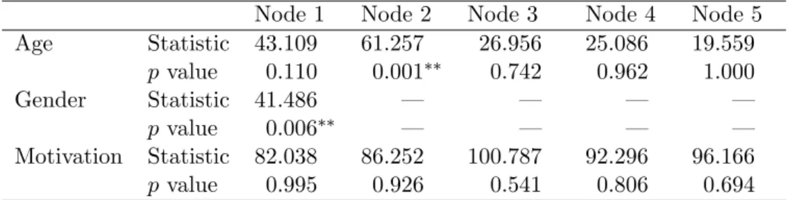
Node 1 Node 2 Node 3 Node 4 Node 5 Age Statistic 43.109 61.257 26.956 25.086 19.559 pvalue 0.110 0.001∗∗ 0.742 0.962 1.000 Gender Statistic 41.486 — — — — pvalue 0.006∗∗ — — — — Motivation Statistic 82.038 86.252 100.787 92.296 96.166 pvalue 0.995 0.926 0.541 0.806 0.694
Table 2: Summary of the parameter instability test statistics and correspondingp values for the instructive example. Those variables whosep values are highlighted with∗∗ symbols are selected for splitting in the respective node.
where ∆qis the increment within theq-th category. This test statistic is invariant to reordering
of the Q categories and the subjects within each category. The test statistic captures the instability over theQsubsamples. Its limiting distribution isχ2with (Q−1)·(m−1) degrees of freedom, from which p values can be computed. This test is employed for both nominal and ordinal categorical variables. A potential ordering of the categories is accounted for in the next step, when the cutpoint is selected (see Section2.3below).
For the Rasch model, the objective function used for parameter estimation is the conditional log-likelihood. The individual contributions to the conditional log-likelihood can be easily computed as logLc(β|ri) (cf. Equation1), yielding
Ψ(ui,β) =− m
X
j=1
uij·βj−log (γri(β)). (5)
For the computation of the structural change tests, the individual contributions to the score function are derived from Equation5. The contribution of the j-the item parameter for the
i-th subject is: ψ(ui,β)j = ∂Ψ(ui,β) ∂βj =−uij − 1 γri(β) ·∂γri(β) ∂βj (6) The derivatives of the symmetric functionsγri(β) are again symmetric functions with certain terms omitted (cf., e.g., Fischer and Molenaar 1995). In our implementation of the Rasch trees, the sum algorithm ofLiou (1994) is used (by default) for computing these derivatives. When the individual contributions to the score function of the Rasch model from Equation6
are ordered with respect to covariate`and inserted in Equation 2, parameter instabilities in the item parameters can be statistically tested using the model-based recursive partitioning approach outlined above.
The results of this procedure are easy to interpret: The parameter instability test statistics
S` with associated p values are provided for each candidate variable, as illustrated for the
instructive example in Table 2. The test statistics for the numeric variable age corresponds to Equation 3 and for the categorical variable gender and the ordered categorical variable motivation to Equation4;p values are derived from the respective limiting distributions. In the first node, the variable with the smallestp value – in this case gender – is selected for splitting (cf. Table2and Figure1). In each daughter node the splitting continues recursively: Here, the variable age is selected for splitting in the second node, whereas no split is found
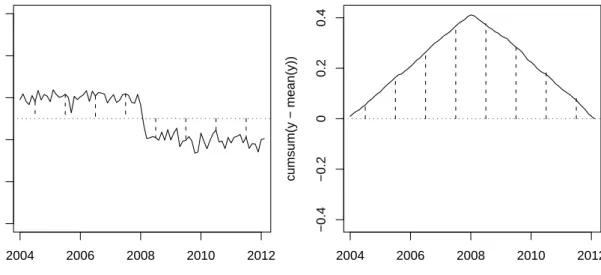
25 30 35 40 45 50 55 60 −950 −945 −940 −935 −930 −925 age log−lik elihood
Figure 3: Log-likelihood of the partitioned Rasch model for the second split in the covariate age. The dashed line indicates the location of the optimal cutpoint (at the value 34) while the dotted line indicates the location of the median (at the value 45).
in the third node. Note that the variable gender is no longer available for splitting starting from the second node as it offers only one possible cutpoint (that has already been used for the first split).
As opposed to gender, the second splitting variable age is numeric and offers as many possible cutpoints as it has distinct values. In this case, it is an important advantage of the model-based recursive partitioning method that the exact cutpoint does not need to be pre-specified, but is determined in a data-driven way as described in detail in the next section.
Splitting continues until allpvalues exceeded the significance level (commonly 5%), indicating that there is no more significant parameter instability, or until the number of observations in a subsample falls below a given threshold. Note that thep values are Bonferroni adjusted as outlined in Section2.4.
2.3. Selecting the cutpoints
After a covariate has been selected for splitting, the cutpoint is determined by maximizing the partitioned likelihood (i.e., the sum of the likelihoods for the observations before and after the cutpoint) over all candidate cutpoints within the range of this variable.
For the first split in the instructive example, this is straightforward as gender only allows for a single split into female and male subgroups. In the second split, however, all possible cutpoints in the variable age for the male subset are considered and the associated partitioned likelihoods are displayed in Figure 3. Clearly the age 34 is the optimal cutpoint, i.e., the strongest difference in the item parameters exists between males up to and over the age of 34.
Note that this cutpoint is obtained directly from the data, whereas standard approaches, such as the graphical or likelihood ratio test, require pre-specified focal and reference groups. For these standard approaches, often the median or mean is used as a cutpoint to split the sample into focal and reference group. However, this choice is completely arbitrary and may even conceal an actual parameter difference related to another cutpoint – as in this example, where the median 45 is far off the maximum indicating the strongest parameter change (cf. Figure3). As a result, using the median as an arbitrarily pre-specified cutpoint may result in an insignificant test result, even though DIF is clearly present in the variable. As opposed to that, the data-driven approach suggested here can detect both whether there is parameter instability with respect to the variable age and where the parameter change occurs.
Formally, for a numeric splitting variable we can define the subsamplesL(ξ) ={i|xi` ≤ ξ}
and R(ξ) = {i|xi` > ξ} on the left and right, respectively, of some cutpoint ξ. For both
subsamples, the parameters βˆ(L) and βˆ(R) can be estimated separately as described above. To determine the optimal cutpoint ξ, the partitioned log-likelihood
X i∈L(ξ) Ψui,βˆ (L) + X i∈R(ξ) Ψui,βˆ (R)
is maximized over all candidate cutpoints ξ (typically requiring a certain minimal subsample size).
While this approach can be applied to numeric and ordered covariates, for unordered cate-gorical covariates theQcategories can be split into any two groups. From all these candidate binary partitions, again the one with the maximal partitioned likelihood is chosen.
What is important to note here is that the optimal cutpoint is determined only if a variable is associated with a significant parameter instability, which prevents variable selection bias (cf., e.g.,Dobra and Gehrke 2001;Shih 2004;Hothorn, Hornik, and Zeileis 2006;Strobl, Boulesteix, and Augustin 2007). In particular, it would be statistically incorrect to assess the significance of an optimal cutptoint using the standard likelihood ratio test (employing itsχ2distribution). The reason is that due to the optimal selection of the cutpoint (i.e., a special type of multiple testing) the asymptotic distribution of the maximally selected likelihood ratio statistic is not
χ2 anymore (Andrews 1993). In fact, the maximally selected Lagrange-multiplier statistic from Equation 3, that is employed in the Rasch tree method, is asymptotically equivalent to the maximally selected likelihood ratio statistic, but avoids reestimating the model. Thus, the Rasch tree approach provides a sound statistical framework for the automatic detection of the variable and cutpoint inducing the strongest DIF.
2.4. Stopping criteria
For creating a Rasch tree, the four basic steps outlined above – (1) estimating the item parameters of a joint model, (2) testing for parameter instability, (3) selecting the splitting variable and cutpoint and (4) splitting the sample accordingly – are repeated recursively until a stopping criterion is reached.
Two kinds of stopping criteria are currently implemented: Splitting continues only as long as significant parameter instability is detected. If there is no (more) significant instability with respect to any of the covariates, the splitting stops. Thus, the significance level – usually set to 5% – serves as the most important stopping criterion.
In addition to that, as a second stopping criterion a minimum sample size per node can be specified. This minimal node-size should be chosen such as to provide a sufficient basis for parameter estimation in each subsample, and should thus be increased when the number of item parameters to be estimated is large. For the instructive example, e.g., a significance level of 5% and a minimal node-size of 20 were employed.
Finally, one should keep in mind that when a large number of covariates is available in a data set, and all those covariates are to be tested for DIF, multiple testing becomes an issue – as with any statistical test for DIF. To account for the fact that multiple testing might lead to an increased false-positive rate when the number of available covariates is large, a Bonferroni adjustment for thep value splitting criterion is applied. Moreover, the recursive partitioning approach forms a closed testing procedure, so that the significance level holds for the entire tree, not only for each individual split. This ensures that DIF is not erroneously detected as an artefact of the number of candidate variables.
3. Application examples
3.1. General knowledge quiz
An online quiz for testing one’s general knowledge was conducted by the weekly German news magazine SPIEGEL in 2009. Overall, about 700,000 respondents participated in the quiz and answered a set of sociodemographic questions. The general knowledge quiz consisted of a total of 45 items from five different topics: politics, history, economy, culture, and natural sciences. For each topic, four different sets of nine items were available, that were randomly assigned to the participants. A thorough analysis and discussion of the original data set is provided inTrepte and Verbeet(2010).
In order to present an application example with a not too heterogeneous sample and a more realistic size for psychological research, we consider only a subsample: university students enrolled in the federal state of Bavaria, who had all been assigned a particular set of questions (questionnaire number 20). This sample still contains 1075 complete cases, that are employed in the following analysis.
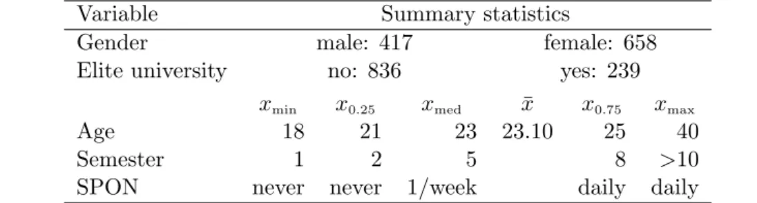
We consider the responses to the 45 quiz items and the covariates gender, age, semester of university enrollment, an indicator for whether the student’s university received elite status by the German “excellence initiative”, and the frequency of accessing SPIEGEL’s online magazine (SPIEGEL Online – SPON). Table3provides summary statistics for these covariates.
Table 3: Summary statistics for the covariates of the general knowledge quiz example.
Variable Summary statistics
Gender male: 417 female: 658
Elite university no: 836 yes: 239
xmin x0.25 xmed x¯ x0.75 xmax
Age 18 21 23 23.10 25 40
Semester 1 2 5 8 >10
The Rasch tree assesses the item responses with respect to the five covariates. As illustrated in Figure4, the Rasch tree has splits in the variables gender, age, and SPON access frequency, indicating DIF in these variables, but not in the variables elite university and semester. Figure 4 also illustrates that it is a combination of the variables gender, age, and SPON access frequency – i.e. an interaction of three variables, rather than one variable alone – that determines which items are easier or harder to solve. With standard approaches, this pattern could only be detected if the interaction terms were explicitly included in the model or the respective groups were explicitly pre-specified. However, in practice usually only DIF in single variables is investigated, so that a complex interaction structure like in this example would not be detected.
Items that show particularly strong DIF include:
The third history item (highlighted by the first large dot: Which form of government is associated with the French King Louis XIV? – Absolutism) is particularly easy for women up to the age of 21 (represented in node 4).
The first economy item (highlighted by the second large dot: Who is this? – Picture of Dieter Zetsche, CEO of Mercedes-Benz) is particularly difficult for women (represented in nodes 4 through 6) and for young men who access SPON up to 2–3 times per week (represented in node 9).
Actually, none of the 118 women represented in node 4 (up to 21 years of age, SPON access up to once per week) answered the item correctly, so that the difficulty parameter could not be estimated and was internally set to infinity (as indicated by the dashed lines pointing out of the range of the plot).
The fourth economy item (highlighted by the third large dot: What is a CEO? – A Chief Executive Officer) is particularly easy for men up to the age of 22 who access SPON more than 2–3 times per week (represented in node 10).
The fifth culture item (highlighted by the fourth large dot: What is the name of the bestselling novel by Daniel Kehlmann? – Measuring The World) is particularly easy for women who access SPON more than once per week (represented in node 6).
The fourth natural sciences item (highlighted by the fifth large dot: What is also termed Trisomy 21? – Down syndrome) is easier for women in general (represented in nodes 4 through 6) and particularly for young women (represented in node 4).
Moreover, it appears that – compared to the other groups – male students over the age of 22 (represented in node 11) find no items particularly easy or particularly hard.
It is also interesting to note that in the general population sample investigated by Strobl, Kopf, and Zeileis(2010a) – as opposed to the student sample considered here – some patterns of DIF coincided with the original subdimensions of the quiz (e.g., history questions tended to be easier for older men), indicating an underlying multidimensionality of the general knowl-edge construct. In our student sample, however, only single items from various topics are particularly easy for students of a certain gender and age, or for those freqently accessing the SPIEGEL online magazine (where it is left to discuss whether the latter should be considered a nuisance dimension, an unfair advantage – or a valid source of general knowledge).
gender p < 0.001 1 female male spon p = 0.004 2 ≤ 1/w eek > 1/w eek age p = 0.013 3 ≤ 21 > 21 Node 4 (n = 118) ● ●● ● ● ● ● ● ● ● ● ● ● ● ● ●● ● ● ● ●● ● ●● ● ● ● ●● ● ● ● ●● ● ● ● ● ● ●● ● ● 1 45 −4 4 Node 5 (n = 169) ● ●●●● ● ● ● ● ● ● ● ● ● ● ●● ● ● ● ●● ● ● ●● ● ●●● ● ● ● ● ● ● ● ● ● ● ● ● ● ● ● 1 45 −4 4 Node 6 (n = 130) ● ●● ● ●● ● ● ● ● ● ● ● ● ●● ● ● ● ●● ● ● ● ● ● ● ● ●● ● ● ● ● ● ●● ● ● ● ● ● ● ● ● 1 45 −4 4 age p < 0.001 7 ≤ 22 > 22 spon p = 0.048 8 ≤ 2−3/w eek > 2−3/w eek Node 9 (n = 176) ● ●● ● ● ● ● ● ●●● ● ● ●● ● ● ●● ●● ● ● ● ●● ● ● ● ● ●● ● ●● ●● ● ● ● ● ● ●● ● 1 45 −4 4 Node 10 (n = 107) ●●● ● ●● ● ●● ● ● ● ● ● ●● ●●● ● ● ● ● ● ● ● ● ● ● ● ● ●● ● ● ● ● ● ● ● ● ● ● ● ● 1 45 −4 4 Node 11 (n = 375) ● ●● ● ● ● ● ● ● ● ● ● ● ● ●● ●● ●● ● ● ● ●● ● ●● ● ●●●● ● ● ●● ● ● ● ● ●● ● ● 1 45 −4 4 ● ● ● ● ● P olitics Histor y Econom y Culture Natur al sciences
Figure 4: Rasch tree for the general knowledge quiz example. The five different colors for the items indicate the five different topics: politics, history, economy, culture and natural sciences.
3.2. Teaching evaluation
The second application example is from the field of teaching evaluation: A questionnaire for evaluating the quality of a lecture was completed by 146 first year students from the faculty of natural sciences at the University of Palermo, Italy, in 2006. The students answered items on the general quality of the lecture, their satisfaction with the lecture, organizational issues, the infrastructure, and the lecturer, as well as some sociodemographic questions. A first analysis and discussion of the full data set is provided byRomano (2010).
The sociodemographic covariates are age, gender, type of residence, number of courses taken during the evaluation phase and job employment. Summary statistics for these covariates are provided in Table4.
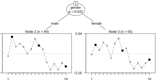
Again, the dichotomized item responses are assessed by the Rasch tree with respect to the five covariates. Seven subjects, for whom all item responses are missing or zero, are excluded from the analysis, leaving 139 observations. As illustrated in Figure 5, the Rasch tree has a split only in the variable gender, indicating DIF between male and female students. No DIF is detected in the variables age, type of residence, number of courses taken and job employment. Items that show particularly strong DIF include:
The second item (highlighted by the first large dot: Were the exam modalities clearly explained in class?) is harder to agree to for male students.
The ninth item (highlighted by the second large dot: Does the timetable allow enough time for changing rooms?) is easier to agree to for female students.
The 16-th item (highlighted by the third large dot: Does the lecturer clearly explain the subject matter?) is harder to agree to for female students.
This example illustrates that DIF can not only occur and be detected in attainment tests, but also in evaluations, as well as attitude or personality tests, where different groups of participants may interpret the items differently or be influenced in their item responses by different dimensions of the latent trait. In any case, whenever one or more splits are found by the Rasch tree, a joint Rasch model – as well as a simple ranking, that also assumes unidimensionality – is no longer appropriate for describing the data.
Table 4: Summary statistics for the covariates of the teaching evaluation example.
Variable Summary statistics Missing
Gender male: 89 female: 54 3
Residence resident: 51 commuter: 35 non resident: 46 14
Job none: 120 part time: 14 full time: 3 9
xmin x0.25 xmed x¯ x0.75 xmax
Age 18 19 19 19.21 19 28 1
gender p = 0.032 1 male female Node 2 (n = 84) ● ● ● ● ● ● ● ● ● ● ● ● ● ● ● ● 1 16 −3.16 3.34 Node 3 (n = 55) ● ● ● ● ● ● ● ● ● ● ● ● ● ● ● ● 1 16 −3.16 3.34
Figure 5: Rasch tree for the teaching evaluation example.
4. Discussion and outlook
We have proposed a new method for detecting DIF that combines the advantages of previous approaches for given groups and latent classes: Groups of subjects exhibiting DIF are auto-matically detected, but remain directly interpretable with respect to their covariate values. In particular, in numeric covariates it is no longer necessary to pre-specify a cutpoint for defining focal and reference groups, but the cutpoint associated with the strongest parameter difference is detected automatically. Thus, DIF in a numeric covariate cannot go unnoticed due to a suboptimal definition of the groups.
When DIF is considered as an indicator of multidimensionality, the graphical display of the Rasch trees can also help identify both groups of items and groups of subjects that may be affected by an additional dimension – whether it be of interest or nuisance.
Of course, any covariate-based approach can only detect all groups of subjects with DIF when all relevant covariates are observable and available for the analysis. In future research, we plan to combine the covariate-based approach presented here with a latent class approach. Then all information available from covariates could be utilized first before a latent class approach is applied in the terminal nodes to detect any remaining heterogeneity.
Moreover, it should be noted that – as with all observational data – a covariate used for splitting should not be interpreted as the causal source of the observed DIF, because the splitting variable may only serve as a proxy for the unobservable or unavailable true cause. In the example of Stout (2002), e.g., that is cited in the introduction of this paper, if DIF is detected between men and women in test items on paragraphs discussing the physical sciences, gender should not be considered as the actual cause of the DIF, but as an indicator of a variety of educational and social influences – such as a lack of reinforcement for female students’ interest in physical sciences – that eventually lead to disadvantages in those items. Technically, we plan to generalize the method to extensions of the Rasch model (such as those proposed byBirnbaum 1968; Fischer 1973; Masters 1982). In particular, it would be
interesting to apply an extension of the Rasch tree method to a 2-parameter logistic model including a location and a guessing parameter, because this would allow the detection of differential guessing behavior in the case of multiple choice items (also investigated by Ben-Shakhar and Sinai 1991andWesters and Kelderman 1991). For these extensions, it is a great advantage of the proposed method that it is not limited to the conditional maximum likelihood approach employed here, but can be generalized to several other estimation approaches. A related method for detecting different preferences between groups of subjects in the Bradley-Terry model is already implemented in thepsychotreepackage (seeStrobl, Wickelmaier, and Zeileis 2010b).
Computational details
Our results were obtained using the R system for statistical computing (R Development Core Team 2010), version 2.11.1, and the add-on package psychotree (Zeileis et al. 2010), version 0.11-1. Both are freely available under the General Public License from the Compre-hensive R Archive Network. A vignette describing the practical application of the method (by replicating the knowledge quiz illustration) is available along with thepsychotreepackage at
http://CRAN.R-project.org/package=psychotree/. The analysis of the instructive data
example is also replicated in the manual for the functionraschtree.
Acknowledgments
Carolin Strobl is supported by grant STR1142/1-1 (“Methods to Account for Subject-Covari-ates in IRT-Models”) from the German Research Foundation (Deutsche Forschungsgemein-schaft). The authors would like to thank Reinhold Hatzinger for important insights stimu-lated by conversations and the R package eRm (Mair and Hatzinger 2007; Mair, Hatzinger, and Maier 2010).
References
Andersen E (1972). “A Goodness of Fit Test for the Rasch Model.” Psychometrika, 38, 123–140.
Andrews DWK (1993). “Tests for Parameter Instability and Structural Change with Unknown Change Point.”Econometrica,61, 821–856.
Ben-Shakhar G, Sinai Y (1991). “Gender Differences in Multiple-Choice Tests: The Role of Differential Guessing Tendencies.”Journal of Educational Measurement,28(1), 23–35. Birnbaum A (1968). “Some Latent Trait Models and Their Use in Inferring an Examinee’s
Ability.” In F Lord, M Novick (eds.), Statistical Theories of Mental Test Scores. Addison-Wesley, Reading.
Breiman L, Friedman JH, Olshen RA, Stone CJ (1984). Classification and Regression Trees. Chapman and Hall, New York.
Cohen A, Bolt D (2005). “A Mixture Model Analysis of Differential Item Functioning.”Journal of Educational Measurement,42(3), 133–148.
de Meij AM, Kelderman H, van der Flier H (2008). “Fitting a Mixture Item Response Theory Model to Personality Questionnaire Data: Characterizing Latent Classes and Investigating Possibilities for Improving Prediction.”Applied Psychological Measurement,32(8), 611–631. den Noortgate WV, De Boeck P (2005). “Assessing and Explaining Differential Item Func-tioning Using Logistic Mixed Models.” Journal of Educational and Behavioral Statistics,
30(4), 443–464.
Dobra A, Gehrke J (2001). “Bias Correction in Classification Tree Construction.” In CE Brod-ley, AP Danyluk (eds.), Proceedings of the Seventeenth International Conference on Ma-chine Learning (ICML 2001), Williams College, Williamstown, MA, USA, pp. 90–97. Mor-gan Kaufmann.
Fischer G (1973). “The Linear Logistic Test Model as an Instrument in Educational Research.” Acta Psychologica,37(6), 359–374.
Fischer G, Molenaar I (eds.) (1995). Rasch Models: Foundations, Recent Developments and Applications. Springer-Verlag, New York.
Gelin MN, Carleton BC, Smith MA, Zumbo BD (2004). “The Dimensionality and Gender Dif-ferential Item Functioning of the Mini Asthma Quality of Life Questionnaire (MiniAQLQ).” Social Indicators Research,68, 91–105.
Hancock G, Samuelsen K (eds.) (2007). Advances in Latent Variable Mixture Models. Infor-mation Age Publishing, Charlotte.
Hothorn T, Hornik K, Zeileis A (2006). “Unbiased Recursive Partitioning: A Conditional Inference Framework.”Journal of Computational and Graphical Statistics,15(3), 651–674. Liou M (1994). “More on the Computation of Higher-Order Derivatives on the Elementary Symmetric Functions in the Rasch Model.” Applied Psychological Measurement, 18(1), 53–62.
Mair P, Hatzinger R (2007). “Extended Rasch Modeling: TheeRmPackage for the Application of IRT Models in R.” Journal of Statistical Software, 20(9), 1–20. URL http://www.
jstatsoft.org/v20/i09/.
Mair P, Hatzinger R, Maier M (2010).eRm: Extended Rasch Modeling. R package version 0.13-0, URLhttp://CRAN.R-project.org/package=eRm.
Masters G (1982). “A Rasch Model for Partial Credit Scoring.” Psychometrika,47(2), 149– 174.
Pedraza O, Graff-Radford N, Smith G, Ivnik R, Willis F, Petersen R, Lucas J (2009). “Differ-ential Item Functioning of the Boston Naming Test in Cognitively Normal African Ameri-can and Caucasian Older Adults.”Journal of the International Neuropsychological Society,
Perkins A, Stump T, Monahan P, McHorney C (2006). “Assessment of Differential Item Functioning for Demographic Comparisons in the MOS SF-36 Health Survey.” Quality of Life Research,15, 331–348.
R Development Core Team (2010). R: A Language and Environment for Statistical Comput-ing. R Foundation for Statistical Computing, Vienna, Austria. ISBN 3-900051-07-0, URL
http://www.R-project.org/.
Rijmen F, Tuerlinckx F, De Boeck P, Kuppens P (2003). “A Nonlinear Mixed Model Frame-work for Item Response Theory.”Psychological Methods,8(2), 185–205.
Romano C (2010). “Determinants of Students’ Teaching Evaluation According to Their Per-formance: An Approach Based on the Relative Importance Metric.” Submitted manuscript. Rost J (1990). “Rasch Models in Latent Classes: An Integration of Two Approaches to Item
Analysis.”Applied Psychological Measurement,14(3), 271–282.
Shih YS (2004). “A Note on Split Selection Bias in Classification Trees.” Computational Statistics & Data Analysis,45(3), 457–466.
Stout W (2002). “Psychometrics: From Practice to Theory and Back – 15 Years of Non-parametric Multidimensional IRT, DIF/Test Equity, and Skills Diagnostic Assessment.” Psychometrika,67(4), 485–518.
Strobl C, Boulesteix AL, Augustin T (2007). “Unbiased Split Selection for Classification Trees Based on the Gini Index.”Computational Statistics & Data Analysis,52(1), 483–501. Strobl C, Kopf J, Zeileis A (2010a). “Wissen Frauen weniger oder nur das Falsche? –
Ein statistisches Modell f¨ur unterschiedliche Aufgaben-Schwierigkeiten in Teilstichproben.” In S Trepte, M Verbeet (eds.), Allgemeinbildung in Deutschland – Erkenntnisse aus dem SPIEGEL Studentenpisa-Test, pp. 255–272. VS Verlag, Wiesbaden.
Strobl C, Malley J, Tutz G (2009). “An Introduction to Recursive Partitioning: Rationale, Application and Characteristics of Classification and Regression Trees, Bagging and Ran-dom Forests.” Psychological Methods,14(4), 323–348.
Strobl C, Wickelmaier F, Zeileis A (2010b). “Accounting for Individual Differences in Bradley-Terry Models by Means of Recursive Partitioning.”Journal of Educational and Behavioral Statistics. To appear.
Trepte S, Verbeet M (eds.) (2010). Allgemeinbildung in Deutschland – Erkenntnisse aus dem SPIEGEL Studentenpisa-Test. VS Verlag, Wiesbaden.
Westers P, Kelderman H (1991). “Examining Differential Item Functioning due to Item Dif-ficulty and Alternative Attractiveness.”Psychometrika,57(1), 107–118.
Woods C, Oltmanns T, Turkheimer E (2009). “Illustration of MIMIC-Model DIF Testing with the Schedule for Nonadaptive and Adaptive Personality.”Journal of Psychopathology and Behavioral Assessment,31, 320–330.
Zeileis A, Hornik K (2007). “Generalized M-Fluctuation Tests for Parameter Instability.” Statistica Neerlandica,61(4), 488–508.
Zeileis A, Hothorn T, Hornik K (2008). “Model-Based Recursive Partitioning.” Journal of Computational and Graphical Statistics,17(2), 492–514.
Zeileis A, Strobl C, Wickelmaier F, Kopf J (2010).psychotree: Recursive Partitioning Based on Psychometric Models. R package version 0.11-1, URL http://CRAN.R-project.org/
package=psychotree.
Affiliation:
Carolin Strobl, Julia Kopf Department of Statistics
Ludwig-Maximilians-Universit¨at M¨unchen Ludwigstraße 33
DE-80539 M¨unchen, Germany
E-mail: [email protected],[email protected]
Achim Zeileis
Department of Statistics Universit¨at Innsbruck Universit¨atsstr. 15
AT-6020 Innsbruck, Austria
2011-01 Carolin Strobl, Julia Kopf, Achim Zeileis: A new method for detecting differential item functioning in the Rasch model
2010-29 Matthias Sutter, Martin G. Kocher, Daniela R¨utzler and Stefan
T. Trautmann: Impatience and uncertainty: Experimental decisions predict
adolescents’ field behavior
2010-28 Peter Martinsson, Katarina Nordblom, Daniela R¨utzler and
Matt-hias Sutter: Social preferences during childhood and the role of gender and
age - An experiment in Austria and Sweden. Revised version forthcoming in
Economics Letters
2010-27 Francesco Feri and Anita Gantner: Baragining or searching for a better
price? - an experimental study. Revised version accepted for publication in
Games and Economic Behavior
2010-26 Loukas Balafoutas, Martin G. Kocher, Louis Putterman and
Matt-hias Sutter: Equality, equity and incentives: an experiment
2010-25 Jes´us Crespo-Cuaresma and Octavio Fern´andez Amador: Business
cycle convergence in EMU: A second look at the second moment
2010-24 Lorenz Goette, David Huffman, Stephan Meier and Matthias Sutter:
Group membership, competition and altruistic versus antisocial punishment: Evidence from randomly assigned army groups
2010-23 Martin G¨achter and Engelbert Theurl:Convergence of the health status
at the local level: Empirical evidence from Austria
2010-22 Jes´us Crespo-Cuaresma and Octavio Fern´andez Amador: Buiness
cycle convergence in the EMU: A first look at the second moment
2010-21 Octavio Fern´andez-Amador, Josef Baumgartner and Jes´us
Crespo-Cuaresma: Milking the prices: The role of asymmetries in the price
trans-mission mechanism for milk products in Austria
2010-20 Fredrik Carlsson, Haoran He, Peter Martinsson, Ping Qin and
Matt-hias Sutter: Household decision making in rural China: Using experiments
to estimate the influences of spouses
2010-19 Wolfgang Brunauer, Stefan Lang and Nikolaus Umlauf:Modeling
2010-17 Boris Maciejovsky, Matthias Sutter, David V. Budescu and Patrick
Bernau: Teams make you smarter: Learning and knowledge transfer in
auc-tions and markets by teams and individuals
2010-16 Martin G¨achter, Peter Schwazer and Engelbert Theurl: Stronger sex
but earlier death: A multi-level socioeconomic analysis of gender differences in mortality in Austria
2010-15 Simon Czermak, Francesco Feri, Daniela R¨utzler and Matthias
Sut-ter:Strategic sophistication of adolescents - evidence from experimental
normal-form games
2010-14 Matthias Sutter and Daniela R¨utzler: Gender differences in competition
emerge early in live
2010-13 Matthias Sutter, Francesco Feri, Martin G. Kocher, Peter
Martins-son, Katarina Nordblom and Daniela R¨utzler: Social preferences in
childhood and adolescence - a large-scale experiment
2010-12 Loukas Balafoutas and Matthias Sutter: Gender, competition and the
efficiency of policy interventions
2010-11 Alexander Strasak, Nikolaus Umlauf, Ruth Pfeifer and Stefan Lang:
Comparing penalized splines and fractional polynomials for flexible modeling of the effects of continuous predictor variables
2010-10 Wolfgang A. Brunauer, Sebastian Keiler and Stefan Lang: Trading
strategies and trading profits in experimental asset markets with cumulative information
2010-09 Thomas St¨ockl and Michael Kirchler: Trading strategies and trading
profits in experimental asset markets with cumulative information
2010-08 Martin G. Kocher, Marc V. Lenz and Matthias Sutter: Psychological
pressure in competitive environments: Evidence from a randomized natural experiment: Comment
2010-07 Michael Hanke and Michael Kirchler: Football Championships and
Jer-sey sponsors’ stock prices: an empirical investigation
2010-06 Adrian Beck, Rudolf Kerschbamer, Jianying Qiu and Matthias
Sut-ter: Guilt from promisebreaking and trust in markets for expert services
environment
2010-04 Martin G¨achter, David A. Savage and Benno Torgler:The relationship
between stress, strain and social capital
2010-03 Paul A. Raschky, Reimund Schwarze, Manijeh Schwindt and
Fer-dinand Zahn: Uncertainty of governmental relief and the crowding out of
insurance
2010-02 Matthias Sutter, Simon Czermak and Francesco Feri: Strategic
sophi-stication of individuals and teams in experimental normal-form games
2010-01 Stefan Lang and Nikolaus Umlauf: Applications of multilevel structured
Working Papers in Economics and Statistics
2011-01
Carolin Strobl, Julia Kopf, Achim Zeileis
A new method for detecting differential item functioning in the Rasch model Abstract
Differential item functioning (DIF) can lead to an unfair advantage or disadvantage for certain subgroups in educational and psychological testing. Therefore, a variety of statistical methods has been suggested for detecting DIF in the Rasch model. Most of these methods are designed for the comparison of pre-specified focal and reference groups, such as males and females. Latent class approaches, on the other hand, allow to detect previously unknown groups exhibiting DIF. However, this approach provides no straightforward interpretation of the groups with respect to person characteristics. Here we propose a new method for DIF detection based on model-based recursive partitioning that can be considered as a compromise between those two extremes. With this approach it is possible to detect groups of subjects exhibiting DIF, which are not prespecified, but result from combinations of observed covariates. These groups are directly interpretable and can thus help understand the psychological sources of DIF. The statistical background and construction of the new method is first introduced by means of an instructive example, and then applied to data from a general knowledge quiz and a teaching evaluation.
ISSN 1993-4378 (Print) ISSN 1993-6885 (Online)