University of South Florida
Scholar Commons
Graduate Theses and Dissertations Graduate School
11-16-2015
An Empirical Comparison of the Effect of Missing
Data on Type I Error and Statistical Power of the
Likelihood Ratio Test for Differential Item
Functioning: An Item Response Theory Approach
using the Graded Response Model
Patricia Rodriguez De Gil
University of South Florida, [email protected]
Follow this and additional works at:http://scholarcommons.usf.edu/etd Part of theEducational Assessment, Evaluation, and Research Commons
This Dissertation is brought to you for free and open access by the Graduate School at Scholar Commons. It has been accepted for inclusion in Graduate Theses and Dissertations by an authorized administrator of Scholar Commons. For more information, please contact
Scholar Commons Citation
Rodriguez De Gil, Patricia, "An Empirical Comparison of the Effect of Missing Data on Type I Error and Statistical Power of the Likelihood Ratio Test for Differential Item Functioning: An Item Response Theory Approach using the Graded Response Model" (2015).Graduate Theses and Dissertations.
An Empirical Comparison of the Effect of Missing Data on Type I Error and Statistical Power of the Likelihood Ratio Test for Differential Item Functioning:
An Item Response Theory Approach using the Graded Response Model
by
Patricia Rodríguez de Gil
A dissertation submitted in partial fulfillment of the requirements for the degree of
Doctor of Philosophy
in Curriculum and Instruction with an emphasis in
Measurement and Evaluation and Secondary Social Science Education Department of Educational and Psychological Studies
Department of Teaching and Learning College of Education
University of South Florida
Co-Major Professor: Jeffrey D. Kromrey, Ph.D. Co-Major Professor: Bárbara C. Cruz, Ed.D.
Eun Sook Kim, Ph.D. James A. Duplass, Ph.D.
Date of Approval: November 10, 2015
Keywords: Validity, Invariance, Civics education, Attitude assessment, Polytomous items
DEDICATION
To my children, with great love.
Adelina Patti Ismael Everardo
ACKNOWLEDGMENTS “Pa’ riba and pa’ lante!”
Alfred North Whitehead said, “No one who achieves success does so without acknowledging the help of others. The wise and confident acknowledges this help with
gratitude”. Never this statement has been more genuine than in this occasion in which I take the opportunity to express my great appreciation and love for those who stood by my side all along this journey. First and foremost, my utmost appreciation goes to my husband, Ismael Gil and to my children. My husband has always been my source of strength; I would not have completed my degree without his constant help and support. My children have been always my greatest blessing and my motivation for continuing my studies. I also want to thank my mother, Elpidia. She had a clear vision of the relevance that having a career has for a woman and worked
tirelessly for providing her daughters with the means to purse one. My mother always instilled and nurtured my desire to pursue a career. I thank her for all the sacrifices she made so I could go to school and earn a degree. I also want to express my appreciation to Dr. Bárbara Cruz. I honestly believe that I would not be celebrating the completion of my degree without her. Over my years as a student, Dr. Cruz has been literally my most enthusiastic, supportive, and caring professor, and I thank her for inspiring me every day. On the same note, Dr. Jeffrey Kromrey has been my advisor since I started my graduate work and I am very appreciative of all his help and guidance for completing my dissertation work. Both Dr. Cruz and Dr. Kromrey as my co-major professors, they were always willing to read my dissertation drafts and provide their valuable
feedback. I also want to thank the faculty of the Social Studies program at USF. The experiences that each professor in the program provided me with made me a better student and a better teacher. I am in debt to Dr. Michael Berson, who always trusted that I could do it. Working under the supervision of Dr. .James Duplass not only helped me develop teaching skills but also importantly, provided me with the collegiate association that I had yearned for so long. I will never forget the thoughtfulness of Dr. Howard Johnston. It was very meaningful to me that always, before starting any conversation, he always asked about my family. Over the years, I have had the fortune of having excellent professors who in a great way molded the person I am today. I would like to acknowledge specially the members of my dissertation committee. I thank them greatly for their sharing with me their expertise and for their guidance completing my dissertation.
My journey, not only academic but in life, would not be the same without my sister Maria del Rosario, my best friend. I truly believe that she is my God’s sent gift; her unconditional love has accompanied me always. She embodies what having a sister is meant. I also feel fortunate for having such a great friends and colleagues. Thanh Pham and Diep Nguyen have been always there, sharing and cheering. I thank them for being always supportive and for their
encouragement. I look forward to continue having them as colleagues and friends.
Lastly, I thank the Lord, for His many gifts, for His always being with me, for protecting me. To God be the glory and honor. Amen.
TABLE OF CONTENTS
LIST OF TABLES ...v
LIST OF FIGURES ... vii
ABSTRACT ... xi
CHAPTER ONE: INTRODUCTION ...1
Overview ...1
Statement of the Problem ...5
Purpose of the Study ...6
Research Questions ...7
Overview of the Study Design ...8
Data Source: The Civics Education Study of 1999 ...9
Significance of Research...10
Limitations and Summary ...12
Definition of Terms...13
CHAPTER TWO: LITERATURE REVIEW ...18
Overview ...18
Test Validation ...18
Missing Data ...20
Rubin’s Missing Data Taxonomy ...21
Data Missing at Random (MAR) ...21
Data Missing Completely at Random (MCAR)...22
Data Missing Not at Random (MNAR) ...22
Missing Data in Likert-Type Scales ...23
Full Information Maximum Likelihood ...25
Multiple Imputation ...26
Single Regression Substitution ...27
Relative Mean Substitution ...27
Person Mean Substitution ...29
Listwise Deletion ...30
Overview of CCT and IRT ...31
Differences between CTT and IRT Item Statistics ...31
Classical Test Theory Item Analysis ...32
Item Response Theory Item Analysis ...36
Trait (θ) ...37
Measuring Scale (θ) ...38
IRT Item Parameters ...40
Local Independence ...47
Model Selection for Attitude Measurement ...48
Attitude Measurement ...48
The Graded Response Model (GRM) ...50
Model Definition ...50
Parameter Invariance ...54
Item Parameter Recovery ...54
Differential Item Functioning ...57
Methods for Detecting Differential Item Functioning ...58
Differential Item Functioning in the Graded Response Model ...58
Overview of the Likelihood Ratio Test for Detecting DIF ...60
A Numerical Example...62
Missing Data and Differential Item Functioning ...63
Previous Studies of the Effect of Missing Data on Differential Item Functioning ...64
Summary ...71
CHAPTER THREE: METHOD ...73
Design of the Simulation Study ...73
Overview of the IEA Civics Education Study ...74
Selection of Subscales...75
Subscale G ...76
Subscale H ...76
Subscale J ...76
Sample and Data Generation ...77
Evaluation of the Data Generation Process ...80
DIF Simulation Study ...81
Between Subjects Factors ...82
Sample Size ...82
Proportion of Missing Observations ...83
Number of Missing Items ...84
Within-Subjects Factors ...84
Missing Data Methods ...84
Ability Group Distributions (Impact) ...84
DIF Magnitude ...85
Computer Software ...85
Missing Data Mechanism (MCAR) ...86
Analytical Plan ...87
Type I Error (Rejection of the Null Hypothesis) ...88
Familywise Type I Error Rate ...89
Overall Distribution of Type I Error Rates ...91
Impact of Study Factors on Familywise Error Rates ...91
Statistical Power...92
Overall Distribution of Statistical Power ...92
Comparison of Statistical Power across MDM ...93
CHAPTER FOUR: RESULTS ...94
Research Question 1: Effect of Missing Data on Type I Error Rates ...95
To What Extent Was the Effect Consistent When α = .01? ... 96
Complete Data ...96
FIML ...96
Multiple Imputation ...98
Person Mean Substitution ...99
Single Regression Substitution ...100
Relative Mean Substitution ...103
Listwise Deletion ...105
Research Question 1 Summary (α = .01) ...106
To What Extent Was the Effect Consistent When (α = .05)? ...108
Complete Data ...110
FIML ...110
Multiple Imputation ...110
Person Mean Substitution ...112
Single Regression Substitution ...112
Relative Mean Substitution ...115
Listwise Deletion ...119
Type I Error Control (Bradley’s Criteria) ...120
Research Question 1 Summary (α = .05) ...124
Research Question 2: Effect of Missing Data on Statistical Power ...125
Power – Bonferroni Adjustment (α = .01) ...126
Power – Bonferroni Adjustment (α = .05) ...131
Research Question 2 Summary ...136
CHAPTER FIVE: DISCUSSION ...137
Criteria for Robustness ...139
The Multiple Significance Testing Problem ...139
Statistical Power in the Context of Multiple Significance Testing ...141
Precision of Simulation Results ...141
Discussion of Findings: Type I Error...143
Discussion of Findings: Statistical Power...147
Last Thoughts: Recommendations and Future Research ...148
REFERENCES ...151
APPENDIX A: TESTING ITEM RESPONSE THEORY ASSUMPTIONS ...162
APPENDIX B: MULTILOG SYNTAX FILES FOR GRM ITEM PARAMETER CALIBRATION CIVICS EDUCATION STUDY (1999) SUBSCALES G, H, J...173 APPENDIX C: ITEM PARAMETER RECOVERY: THE EFFECT OF SAMPLE
SIZE, NUMBER OF ITEMS, NUMBER OF REPLICATIONS AND MISSING DATA METHODS ON THE RECOVERY OF THE GRADED RESPONSE MODEL
APPENDIX D : SUMMARY TABLES: EFFECT SIZE ESTIMATES FOR TYPE I
ERROR AND POWER...199 APPENDIX E: IRB HUMAN SUBJECTS DETERMINATION AND IRB
LIST OF TABLES
Table 1: Classical Test Theory Item Analysis ...33
Table 2: Classical Test Theory Item Analysis ...39
Table 3: Critical Chi-Square and Critical Bonferroni Values ...62
Table 4: Results for an IRT-LR Test Using Graded Responses with Five Response Categories ...63
Table 5: Survey Scales for the Civics Education (CivEd) Study ...75
Table 6: True Item Parameter Estimates ~N(0,1) ...78
Table 7: Missing Data Simulation Matrix ...82
Table 8: Item Parameter Modification to Simulate DIF ...85
Table 9: Rejection Criteria: Adjusted P, and χ2 and Bonferroni Critical Values ...89
Table 10: Hypothesis Testing in the Context of Multiple Testing for Multiple Imputation ...91
Table 11: Proportion of Conditions with Adequate Type I error Control ...121
Table 12: Mean power estimates by method and DIF for Bonferroni adjustment .01...127
Table 13: Mean power estimates by method and DIF for Bonferroni adjustment .05...133
Table A1: Test Statistics for Subscales G, H, and J ...162
Table A2: Summary of Frequencies, Means, and Standard Deviations ...165
Table C1: Frequency Distributions of Items’ Category Options by Subscale J ...178
Table C2: Frequency Distributions of Items’ Category Options by Subscale H ...179
Table C3: Frequency Distributions of Items’ Category Options by Subscale G ...181
Table C5: Mean RMSE Estimates by Sample Size across Replications ...196 Table D1: Main and First-Order Interaction Effects on Familywise Error Rates ...195 Table D2: Main and First-Order Interaction Effects on Statistical Power ...195
LIST OF FIGURES
Figure 1: Item Characteristic Curve or ICC for a dichotomous item ...42
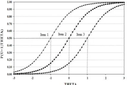
Figure 2: Item Characteristic Curve (ICC) for three items differing in difficulty parameter...43
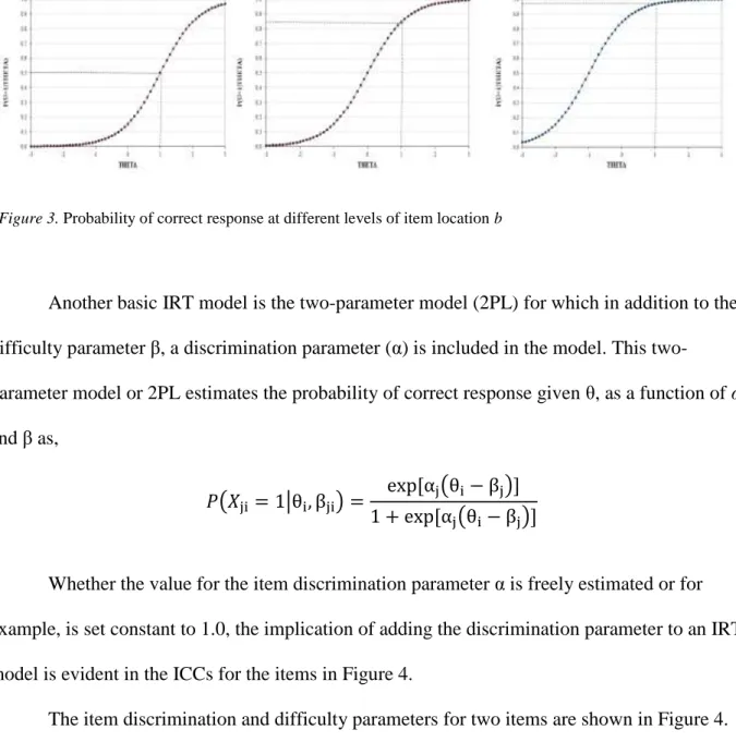
Figure 3: Probability of correct response at different levels of item location ...45
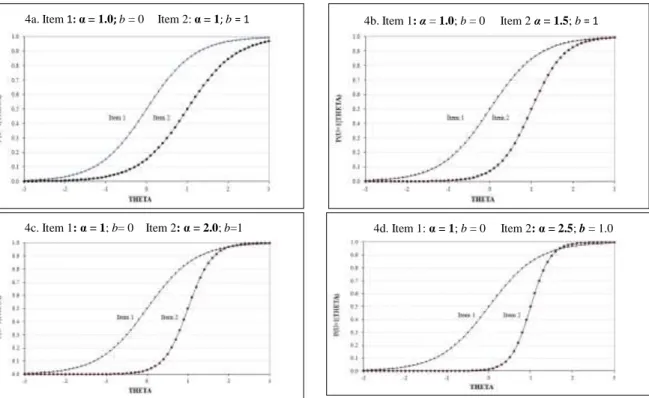
Figure 4: Item discrimination parameter varying by .5 across graphs ...46
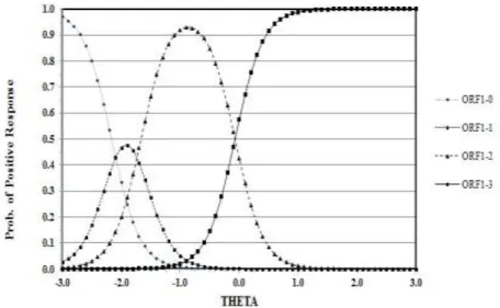
Figure 5: Option Response Function (ORF) for a graded item with four categories ...52
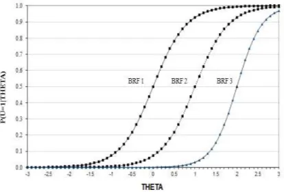
Figure 6: Boundary Response Function (BRF) for a 4-option item ...53
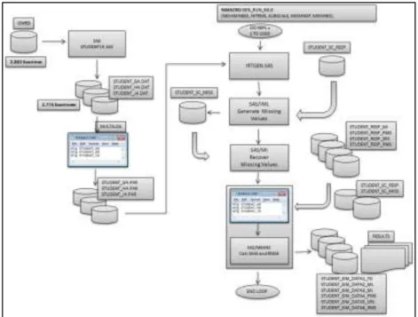
Figure 7: Flow process from accessing the CivEd data for the national sample ...81
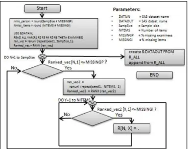
Figure 8: MCAR missing data generation ...87
Figure 9: Overall familywise error rate distributions (α = .01) ...95
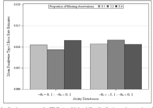
Figure 10: Mean familywise error rates for FIML (α = .01) ...97
Figure 11: Mean familywise error rates for MI (α = .01) ...98
Figure 12: Mean familywise error rates for SRS (α = .01)...100
Figure 13: Mean familywise error rates for SRS (α = .01)...101
Figure 14: Mean familywise error rates for SRS (α = .01)...102
Figure 15: Mean familywise error rates for RMS (α = .01) ...103
Figure 16: Mean familywise error rates for RMS (α = .01) ...104
Figure 17: Mean familywise error rates for RMS (α = .01) ...105
Figure 18: Mean familywise error rates for Listwise deletion (α = .01) ...106
Figure 20: Mean familywise error rates for MI (α = .05) ...111
Figure 21: Mean familywise error rates for SRS (α = .05)...113
Figure 22: Mean familywise error rates for SRS (α = .05)...114
Figure 23: Mean familywise error rates for SRS (α = .05)...115
Figure 24: Mean familywise error rates for RMS (α = .05) ...116
Figure 25: Mean familywise error rates for RMS (α = .05) ...117
Figure 26: Mean familywise error rates for RMS (α = .05) ...118
Figure 27: Mean familywise error rates for Listwise deletion (α = .05) ...119
Figure 28: Proportion of conditions with adequate Type 1 error control (α = .01) ...122
Figure 29: Proportion of conditions with adequate Type 1 error control (α = .05) ...123
Figure 30: Overall distribution of power estimates by method (α = .05) ... 126
Figure 31: Mean power estimates for complete data (α = .05)...128
Figure 32: Mean power estimates for FIML (α = .05) ...128
Figure 33: Mean power estimates for PMS (α = .05) ...128
Figure 34: Mean power estimates for RMS (α = .05) ...128
Figure 35: Mean power estimates by number of items for Listwise deletion ...130
Figure 36: Mean power estimates by sample size for Listwise deletion ...130
Figure 37: Mean power estimates by proportion of missing observations ...131
Figure 38: Overall distribution of power estimates by method (α = .05) ...132
Figure 39: Mean power estimates for complete data ...134
Figure 40: Mean power estimates for FIML ...134
Figure 41: Mean power estimates for PMS ...134
Figure 43: Mean power estimates for RMS ...134
Figure A1: Item ORF’s and fit plots for scale G items 1 to 3 ...166
Figure A1: Item ORF’s and fit plots for scale G items 4 to 6 ...167
Figure A2: Item ORF’s scale H (5 items) ...168
Figure A2: Item ORF’s and fit plots for scale H items 4 and 5 ...169
Figure A3: Item ORF’s and fit plots for scale J items 1 to 3 ...170
Figure A3: Item ORF’s and fit plots for scale J item 4 ...171
Figure C1: Scale G distributions for discrimination parameter a1 ...183
Figure C2 Scale G distributions for location parameter b1 ...183
Figure C3: Scale G distributions for location parameter b2 ...184
Figure C4: Scale G distributions for location parameter b3 ...184
Figure C5: Scale H distributions for discrimination parameter a1 ...185
Figure C6 Scale H distributions for location parameter b1 ...185
Figure C7: Scale H distributions for location parameter b2 ...186
Figure C8: Scale H distributions for location parameter b3 ...186
Figure C9: Box plots BIAS distributions for discrimination parameter a ...187
Figure C10: Box plots BIAS distributions for location parameter b1 ...187
Figure C11: Box plots BIAS distributions for location parameter b2 ...188
Figure C12: Box plots BIAS distributions for discrimination parameter b3 ...188
Figure C13: Mean bias distributions for discrimination parameter a ...189
Figure C14: Mean bias distributions for discrimination parameter b1 ...189
Figure C15: Mean bias distributions for discrimination parameter b2 ...190
Figure C17: Box plots RMSE distributions for discrimination parameter a ...191
Figure C18: Box plots RMSE distributions for location parameter b1 ...191
Figure C19: Box plots RMSE distributions for location parameter b2 ...192
Figure C20: Box plots RMSE distributions for discrimination parameter b3 ...192
Figure C21: Mean RMSE distributions for discrimination parameter a ...193
Figure C22: Mean RMSE distributions for discrimination parameter b1 ...193
Figure C23: Mean RMSE distributions for discrimination parameter b2 ...194
ABSTRACT
In the context of educational research, missing data arise when examinees omit or do not reach an item, which generates an item nonresponse problem. Using a simulation approach, in addition to conducting complete data analyses, this study compared the performance of six methods for treating item nonresponse in the context of differential item functioning (DIF). The effect of missing data on the Type I error and statistical power of the Likelihood Ratio test for DIF detection in small scales was examined in the context of Item Response Theory (IRT-LR), using polytomous, Likert-type data and the graded response model. The effect of ability
distribution, sample size, number of items, proportion of missing observations, and proportion of missing items on Type I error rates and empirical power of the IRT-LR DIF test were examined under full information maximum likelihood (FIML), multiple imputation (MI), person mean substitution (PMS), single regression substitution (SRS), relative mean substitution (RMS), and Listwise deletion missing data methods. Type I error rates were very consistent across nominal levels and factors, under each missing data method. Among the missing data methods examined, the FIML and PMS methods had Type I error rates comparable to the rejection rates for complete data. Although MI is considered a “state-of-the-art” missing data method, in this study, MI, as well as SRS were the less effective missing data methods (i.e., both MI and SRS had inflated rejections rates across all conditions). On the same note, Listwise deletion has been described as one of the most ineffective methods; however, under large data, the data loss due to
present, such as a small proportions of missing observations and small number of items or variables. Along with complete data and FIML, the PMS method had an adequate Type I error control under both nominal levels examined. MI and SRS had the smallest proportions of
conditions meeting Bradley’s criteria for robustness at both levels of significance examined; as a result, when alpha was .01 none of the simulation conditions of these methods met the criteria for robustness and were not included in power analyses at this significance level. Power analyses were entirely consistent across nominal levels, factors and missing data methods. Entirely consistent with theory, sample size and proportion of missing observations were the factors affecting the performance of the IRT-LR test for DIF detection across all missing data methods.
CHAPTER ONE INTRODUCTION
“Providing information to test takers and test score users about the abilities of test takers at different score levels has been a persistent problem in educational and psychological
measurement.” — Sinharay, Haberman, and Lee, 2011, p. 61 Overview
The measurement of individuals’ traits, or mental properties such as abilities and attitudes, has been a long-lasting quest that dates back to 1882 with Galton’s pioneering work developing rating scales and questionnaires, and Thorndike’s contributions to psychometric theory and its application to educational measurement (Ward, Stoker, & Murray-Ward, 1996). This quest continues today (Sijtsma & Junker, 2006). But why do we measure individuals’ traits?
Currently, the measurement of students’ academic achievement has a prominent position in the No Child Left Behind (NCLB) Act of 2001 (NCLB, 2002; US Department of Education, 2002), influencing not only classroom practices but also testing at state and national levels. For example, in agreement with Tyler’s (1951) ideas on the influence of educational measurement in the improvement of instruction, Carey (2001) stated that measurement in educational settings serves several purposes, namely, planning, monitoring, and evaluating instruction. Moreover, achievement data influence educational decision making. That is, in addition to improving teaching and learning, the information that test scores provide greatly impacts the classification, selection, placement, and promotion of test takers (Clauser & Mazor, 1998; Garcia & Pearson, 1994). Therefore, empirical evidence should support the validity of inferences from test scores.
At the core of assessment-driven educational reforms such as the NCLB (2002) is the development of methods for eliminating nonrandom, systematic errors in measurement that arise when students with the same ability or trait but from different groups (e.g., male, female;
minority, nonminority) do not have the same probability of answering correctly or endorsing a test item, after the item has been conditioned on ability or trait level (Balsis, Gleason, Woods & Oltmanns, 2007; Embretson & Reise, 2000). Because precision of measurement is required so that it allows for valid interpretations of test scores (Cronbach & Gleser, 1965; Kane, 1996), the focus of extensive research has been the development and improvement of item and test
evaluation procedures that ensure the accurate measurement of students’ ability and traits and consequently, the validity of the interpretation of test scores (Robitzsch & Rupp, 2009). One of these item evaluation procedures is differential item functioning (DIF), which “has become an essential aspect of the validation of test score interpretations” (Ankenmann, Witt, & Dunbar, 1999, p. 278). The Standards for Educational and Psychological Testing (American Educational Research Association, American Psychological Association & National Council of Measurement in Education, 1999), hereafter the Standards, states that:
When credible research reports that differential item functioning exists across age, gender, racial / ethnic, cultural, disability, or linguistic groups in the population of test takers in the common domain measured by the test, test developers should conduct appropriate studies when feasible. Such research should seek to detect and eliminate aspects of test design, content, and format that might bias the test score for particular groups. (p. 81)
That is, when the members of a subgroup of students taking a test do not have the same probability of responding correctly to or endorsing an item as the members of another subgroup of students with the same ability or trait, we say that DIF is present. DIF suggests that the internal structure of tests items (i.e., item parameters’ properties or characteristics such as item discrimination and item difficulty) is not the same for different groups matched on ability (Woods, 2008).
Regardless of this extensive research on the improvement of item and test evaluation procedures, empirical evidence of the disparities in test performance across subgroups of students continue to be a concern well documented in the literature, e.g., gender differences in language achievement (Mullis, Martin, Gonzalez, & Kennedy, 2003), gender differences in mathematics and science achievement (Mullis, Martin, Gonzalez, & Chrostowski, 2004), and gender differences in civic knowledge (Baldi, Perie, Skidmore, Greenberg, & Hahn, 2001).
This increased interest in subgroups’ differences in test scores has resulted in the
development of theories that pose the responsibility of the lower test scores of minority students on external factors to the tests (Hulin, Drasgow, & Komocar, 1982). Such attempts to explain the lower mean test scores of minorities students, for example, rule out differences between groups a
priori (Thorndike, 1971), or pose the responsibility of lower test scores on the minority groups
themselves, within their genetic heritage (Jensen, 1969) and home environments (McPhee, Kreutzer, & Fritz, 1994). Other explanations focus primarily on the role of society and schools (Coleman, 1966), and on the range of variables such as racial discrimination, prejudice, and stereotype that can stigmatize and contribute to the alienation of minority students. However, these external factors are not necessarily evidence of DIF.
There are several statistical methods for identifying differentially functioning test items, each with its strengths and limitations. Some methods are based on classical test theory (CTT) and other methods are based on item response theory (IRT) and the decision on which
framework and procedure are to be implemented, should be taken within the theoretical and empirical specifics of each research situation. The application of CTT and IRT models for dichotomously scored items for the measurement of student achievement and the evaluation of DIF has dominated since early educational testing (Camilli & Shepard, 1994; Clauser & Mazor, 1998; De Ayala & Sava-Bolesta, 1999; Kim, Cohen, Alagoz, & Kim, 2007; Lane, Stone,
Ankenmann, & Liu, 1995). However, it is important to consider also noncognitive assessments because they “influence, in either facilitative or debilitative ways, both student learning and test performance” (Messick, 1984, p. 215). Attitude measurement, for instance, has been a
cornerstone in empirical research (Thissen, Steinberg, Pyszcznski, & Greenberg; 1983) and evidence of validity is equally important for such measures. Furthermore, the current popularity of performance assessments has increased the use of polytomous IRT models e.g., partial credit model (PCM; Masters, 1982), generalized partial credit model (GPCM; Muraki, 1992), and graded response model (GRM; Samejima, 1969, 2010).
Ankenmann et al. (1999) stated that “the detection of differential item functioning (DIF) in polytomously scored, constructed-response items that constitute most performance
assessments has become an essential aspect of the validation of test scores interpretations” (p. 278). However, the use of polytomously scored items does not preclude the potential for differentially functioning items. In addition, the detection of DIF might be complicated by the presence of a pervasive problem in empirical research, that of missing data. In educational testing, missing data occur when a student either does not respond to an item or question (i.e.,
item nonresponse) or does not respond to any question at all (i.e., unit nonresponse). That is, data are missing for some test items, and / or for some students.
When students do not answer items in a test because they do not know the answer, do not have time to respond to all questions, or omit the questions they are not comfortable with (such as in the case of attitudinal measurement), the item nonresponse generates a missing data problem (e.g., the variable of interest and the omitted response are not independent) which cannot be ignored (i.e., leaving data untreated, doing nothing about it). Because the statistical methods used to analyze item responses so that items can be evaluated for DIF might not be robust to missing data (e.g., failure to converge; Drasgow, Levine, Tsien, Williams, & Mead, 1995), data should be treated by applying missing data methods (MDM) that impute plausible values and replace missing data. Then, analyses can be conducted on complete data using standard statistical methods for evaluating DIF.
The crucial question is then, should we care about item nonresponse while doing a DIF analysis? The answer is yes if there is the risk of potential statistical bias associated with valid inferences of test scores and their use.
Statement of the Problem
The development of test validation procedures has led to the study of DIF. However, DIF analyses are potentially subject to spurious interpretations due to the presence of missing data. Depending on the missingness mechanism (i.e., types of missing data), the magnitude of the missing data (i.e., percentage of missing responses for a person and by item), sample size (i.e., number of students taking the test), number of test items (i.e., test length), and the magnitude of DIF (i.e., negligible, moderate, and high), the MDM used to treat the existing missing data due to
item nonresponse might result in data handling complications such as 1) reduced sample size (Davey, Savla & Luo, 2005; O’Rouke, 2003; Zhang, 2003), 2) reduction of analytical power (Yenduri & Iyengar, 1994), and 3) seriously statistically biased results due to the systematic differences between the observed and non-observed data (Little, 1988). In addition to the extent to which item nonresponse might impact the accuracy and precision of the point estimates (i.e., item difficulty and item discrimination parameter estimation), the implementation of a MDM might also impact the performance of the methods used to detect DIF items.
Purpose of the Study
The validity of test score interpretations is closely tied to how the test scores are used (e.g., selection of students). Thus, it is important to state the scope or focus of this study, which is on the internal properties of test items and how these properties might be impacted by the presence of missing data.
Missing data have been broadly explored in the context of statistical methodology such as structural equation modeling (SEM; Gold & Bentler, 2000), and multiple regression
(Brockmeier, Kromrey, & Hogarty, 2003; Kromrey & Hines, 1994). However, there is relatively less research on the effect of missing data on DIF analysis for polytomous data within the IRT framework, compared to research on achievement and binary data. Because much less is known about noncognitive tests such as attitude measurement and because both item nonresponse and MDM play an important role in the performance of a given DIF detection method, the purpose of this study was, within the context of IRT, to empirically compare the effects of six MDM (a maximum likelihood based method, single regression substitution (SRS), relative mean substitution (RMS), person mean substitution (PMS), multiple imputation(MI), and Listwise
deletion) on the Type I error rates and statistical power of the Likelihood Ratio (IRT-LR) test for DIF detection in attitude measurement, using the graded response model (GRM) for polytomous items.
Research Questions
1. What is the effect of missing data (i.e., item nonresponse) and their treatment on the Type I error rate of the Likelihood Ratio test for Differential Item Functioning detection?
a. To what extent is the effect consistent across levels of significance? b. To what extent is the effect consistent across MDM?
i. To what extent is the effect consistent across sample size?
ii. To what extent is the effect consistent across percentage of missing data by persons and items?
iii. To what extent is the effect consistent across the magnitude of DIF? iv. To what extent is the effect consistent across population distributions? 2. What is the effect of missing data and their treatments on the statistical power of the
Likelihood Ratio test for Differential Item Functioning detection?
a. To what extent is the effect consistent across levels of significance? b. To what extent is the effect consistent across MDM?
i. To what extent is the effect consistent across sample size?
ii. To what extent is the effect consistent across percentage of missing data by persons and items?
iii. To what extent is the effect consistent across the magnitude of DIF? iv. To what extent is the effect consistent across population distributions?
Overview of the Study Design
The research questions were addressed using a simulation approach in which a crossed factorial design was used to investigate the effect that missing data or item nonresponse and MDM had on the effectiveness of the IRT-LR test for detecting DIF in the GRM, in terms of Type I error and statistical power. The factors manipulated in the simulation study included population distributions for the reference and focal groups θR ~ N(0,1) : θF ~ N(0,1), and θR ~
N(0,1) : θF ~ N(-.5,1), total sample size (N1=500 and N2=1000) in the following ratios: 1:1, and 3:2 for the reference and focal groups respectively (nR=250 : nF=250, nR=500 : nF=500, and
nR=300 : nF=200, nR=600 : nF=400), number of items or test length (4-, 5-, and 6-items scales, with 4 response Likert-type categories in each item), proportion of missing observations or persons (10%, 20%, 40%) , proportion of missing items (~20% and ~40% or 1 and 2 items respectively), and magnitude of DIF (.25, .50 and .75). Nominal levels of alpha for the test of the null hypothesis were .01 and .05. For each combination of conditions, 1000 samples or number of replications (nR) were generated. The use of 1000 samples or replications provided a
maximum standard error of .015 and a 95% confidence interval width ± .03 around observed rates of Type I error (Robey & Barcikowski, 1992). The proposed MDM were applied and their effect on the Type I error rates and statistical power of the IRT-LR test for DIF were estimated. Bradley’s liberal criterion (1978) was used for the evaluation of robustness of Type I error control at α= .01 and α = .05; power analyses were conducted for those conditions evidencing adequate Type I error control (Ankenmann et al., 1999). In addition, complete data analyses were conducted for comparison purposes.
Data Source: The Civics Education Study of 1999
Data for this study was generated using item parameters’ values estimated from three subscales included in the survey section of the Civics Education Study of 1999 (U.S. Department of Education, National Center for Education Statistics, 1999). Considering the broad range of restricted data and publicly available data, why selecting data from the social studies framework?
To achieve quality education in American schools, a better understanding of how classroom instruction work is needed (Stodolsky, 1988). Social studies as a school subject matters; Yeager and Davis (2005) stated, for example, that “social studies is a potentially powerful, engaging, and relevant curriculum area” (p. 2). However, as federal and
state-mandated assessment has elevated the status of mathematics, sciences, and reading literacy core subjects, the study of the social sciences, also a core subject, has been relegated as an
“enrichment” subject matter with a limited allocation of instructional time in elementary level (Brophy & VanSlendright, 1997), and reduced to the irrelevant teaching of facts in middle and secondary levels (Vogler & Virtue, 2007). Has placing the social studies in the “back burner” (Vogler, Lintner, Lipscomb, Knopf, Heafner & Rock, 2007) made middle school students passive recipients of current global realities? What do young people think about democracy? Do they understand how democratic institutions work? Do they expect to vote and to take part in other civic activities as adults? These are the questions that motivated the Civics Education study of 1999 and if we are to understand how schools and social studies classroom instruction
prepares our young students for participating in our democratic institutions, promoting civic knowledge, attitudes, and involvement, it is important that the instruments used to measure students’ attitudes toward those institutions are valid. This is basically what the subscales selected for this study address and what make them worth to study.
Thus, this study was conducted using item parameters estimated from three subscales of the Civics Education Study measuring students’ degree of adherence to common values and attitudes toward women’s rights, immigration, and political activism. In addition to the advantage of conducting the simulation study by generating data that emulate the conditions under study, using real data provided the additional advantage of carrying the study under normally occurring violation of assumptions (e. g., normality of distributions; Kromrey and Hines, 1994).As this international study was conducted in 28 countries; the item parameters for this study were estimated from the United States public data sample for the standard population (9th grade students; N=2811). The study was conducted using SAS 9.4 and the IRTGEN SAS macro (Whittaker, Fitzpatrick, Williams, & Dodd, 2003) was used to generate data to conform the GRM. The item parameters were calibrated using the marginal maximum likelihood estimation method, as implemented in MULTILOG 7.03 (Thissen, 2003).
Significance of Research
Previous to the legislation of the NCLB (2001), any mandated testing did not have any consequences for poorly performing students and schools. But with the implementation of the NCLB, not only testing dramatically increased (e.g., the NCLB mandates the administration of 17 tests (personal communication with Dr. Bárbara Cruz, May 4, 2015)) but also, testing steered toward accountability for those not meeting the goals of the NCLB. How students and schools are held accountable is observed in the mounting role of standardized testing (e.g., American students are tested far more than students in other countries) and in the sanctioning of low
performing schools. However, as John Merrow (2001) asserted, tests are not evil. Andrich (2002) said that, “Assessment should be valid, educative, explicit, fair, and comprehensive” (p. 105).
Thus, the quality of measurement instruments has drawn the attention not only of test developers but also of scholars from many disciplines, policy makers, and administrators (Cizek, 2012). However, the interpretation of test scores must be placed in the overall test development procedure, not just on the total score. As Linn (1990) stated, “the most important question
regarding any measure concerns the validity of the uses and interpretation of the scores” (p. 115). Despite the continued development of test validation procedures (e.g., DIF studies), the presence of systematic measurement errors (measurement bias) that arise when factors other than the underlying construct are measured is a threat to the validity of the inferences from test scores (Zumbo, 1999). The relevance of validity in test score interpretations is captured in its references as being “one of the major deities in the pantheon of the psychometrician” (Ebel, 1961, p. 640) and as “the foundation for virtually all of our measurement work” (Frisbie, 2005, p. 21). Yet, as Cizek (2012) stated, “all is not well with validity” (p. 31). DIF continues to be a threat to validity and while the psychometric basis of tests has changed dramatically (Embretson & Reise, 2000; Hambleton & Slater, 1997; Linn, 1990) and several school reforms have been implemented in response to these problems, missing data and DIF are ubiquitous in empirical research and both pose a serious threat to the fairness in test use and validity of the interpretation of test scores.
Su and Wang (2005) stated, “The detection of differential item functioning (DIF) in polytomous items has attracted much attention in recent years” (p. 313). However, most IRT work has been based on dichotomous models (De Ayala & Sava-Bolesta, 1999) and currently, there is still a predominance of achievement testing using binary item formats. Testing relying on dichotomously scored items can be a disadvantage (Dodd, Koch, De Ayala; 1989); thus, a better option is to use a model that assesses information across all item categories (De Ayala & Sava-Bolesta, 1999) as is the case in polytomous models.
Because of the dominance of achievement testing and the application of objective tests, much less is known about other types of measurement using noncognitive data, as is the case of attitude assessment that is also part of the process through which students construct knowledge and develop abilities. Polytomous data, collected in the form of graded responses can be used to address and provide insights on attitudinal aspects that affect student academic achievement. Thus, evidence of the validity of these measures is equally important (Ankenmann et al., 1999).
Limitations and Summary
A limitation of simulated data studies is that the data generation process and methods might apply only to the conditions under study (e.g., data generation methods might favor the IRT method used for bias detection). Also, the study will use self-reported measures of attitudes which can be problematic due to, for example, providing a socially desirable response.
In this chapter, the purpose of the study was introduced along with the problem in making valid inferences from test scores, and the problems that missing data generate in the detection of differentially functioning test items. Issues of differential item functioning in measurement were introduced and its impact in students’ selection and classification was discussed. The
implementation of a simulation study was elaborated and the use of item response theory (IRT) and specifically, the GRM, was justified. The next chapter provides a literature review on missing data in Likert-type scales, and on IRT and its implementation in the detection of
differentially functioning items or DIF. In addition, the analytical plan was developed in chapter III.
Definition of Terms
Ability: It refers to the ability or trait being measured and within item response theory is
represented by the Greek small letter Theta (θ). Thus, the ability for examinee i, is represented as θi. In educational research, the value of ability or trait is assumed to be unknown and hence,
estimated (Harwell, Baker, & Zwarts, 1988). Although the terms are not synonymous, ability can also be referred or used interchangeably as proficiency (Osterlind & Everson, 2009).
Accuracy: Degree of closeness of measurements of a quantity to the actual or true value.
In this context, Bias is a statistical index of the accuracy of measurement (Mellenbergh, 1989).
Bias: It refers to statistical bias or the difference between the average value of the
estimated parameter across simulation replications and its true value (DeMars, 2003; Stone, 1992; Wang & Chen, 2005).
Construct (psychological): Postulated attribute of people, assumed to be reflected in test
performance (Cronbach & Meehl, 1955). Thus, a construct is an unobserved, latent variable underlying behavior and “imperfectly measured by a test or questionnaire” (Embretson & Reise, 2000; Schafer & Graham, 2002).
Dichotomous item: An item is a dichotomous item if it is scored with two response
categories such as yes/no, correct/incorrect, or agree/disagree (Cohen, Kim, & Baker, 1993; Clauser & Mazor; 1998).
Differential Item Functioning (DIF): Differences in the functioning of an item among
groups that are matched on the attribute measured by the item (Clauser & Mazor, 1998; Cohen et al., 1993; Paek & Guo, 2011). When a test item favors one group over another, the item exhibits DIF.
Spurious DIF: Identification of DIF in an item due to the method used. Andrich and Hagquist (2012) also termed this type of DIF as Artificial DIF.
Unbiaseditem: Item for which the probability of a correct response is the same for all
persons of a given ability, regardless of their ethnic, cultural, sex, or group membership (Cohen et al., 1993). On the other hand, a biased item or item bias is one that unfairly favors one group over another (Clauser & Mazor, 1998). In IRT, an item is considered biased “when it differs in difficulty between subjects of identical ability from different groups” (Mellenbergh, 1989, p. 128).
UniformDIF: When examinees of a subgroup taking a test consistently have higher
probability of answering correctly an item, we say that the item presents uniform (i.e., constant difference across all levels of ability measured by the test) differential functioning (Mellenbergh, 1982).
Item difficulty (β): Item technical property or descriptor. In CTT, item difficulty is the
proportion of examinees of the total group that responded correctly to an item. In IRT and binary items, item difficulty or location parameter, specifies the point in the ability scale at which the probability of an examinee of responding correctly or selecting an item response is .50. Because β indicates where an item functions on the ability scale, within IRT it is a location index (Baker, 1977; Embretson and Reise, 2000).
Item discrimination (α): Item technical property or descriptor. Determines how well the
item differentiates between examinees whose ability is below the item location and those having ability above the item location.
Itemimpact: Refers to the differences in the performance of groups of examinees on
item; that is, it is the true difference in performance of groups of examinees with different abilities on specific items (Clauser & Mazor; 1998; Robitzsch & Rupp, 2009).
No DIF item: The expectation for valid test score comparisons is that items’ structural
properties are the same among test takers having the same standing on the trait being measured. Thus, a No DIF item is one that is invariant across groups so that “the expected value of a response to the item from persons from different identifiable groups is the same” (Andrich & Hagquits, 2012, p. 387).
False Negative (FN): Failure of detection in the presence of the condition being tested for
(also known as Type II error or β, the probability of failing to reject the null hypothesis when the null hypothesis is false). In DIF studies, identifying an item as being free of DIF (NO DIF item) when the item is a DIF item (Andrich & Hagquits, 2012).
True Negative (TN): Failure of detection in the absence of the condition being tested for
(i.e., failure to reject the null hypothesis when the null hypothesis is true). In DIF studies, identifying a DIF free item as a DIF free (Andrich & Hagquits, 2012).
False Positive (FP): Incorrect detection in the absence of the condition being tested for
(also known as Type I error or α, the probability of rejecting the null hypothesis when the null hypothesis is true). In DIF studies, FP means identifying an item as a DIF item when the item does not show DIF (Andrich & Hagquits, 2012).
True Positive (TP): Correct detection in the presence of the condition being tested for
(also known as power; rejection of the null hypothesis when the null is false). In DIF studies, a DIF item is correctly identified as a DIF item (Andrich & Hagquits, 2012).
Trait: Messick (1989) defines a trait as “a relative stable characteristic of a person—an
attribute, enduring process, or disposition—which is consistently manifested to some degree when relevant, despite considerable variation in the range of settings and circumstances” (p. 15).
Likert-type scale: psychometric scale commonly involved in research that employs
questionnaires. It is the most widely used approach to scaling responses in survey research.
Likelihood Ratio test (LR): Statistical test used to compare the fit of two models, one of
which (the null model) is a special case of the other model (the alternative model). The test is based on the likelihood ratio, which expresses how many times more likely the data are under one model than for the other model.
Measurement: Procedure with which a number is assigned to an object of measurement
to represent the value of some attribute for that object of measure (Kane, 1996).
p: The proportion of correct responses to the total number of responses of people scoring within that range. At the item level, Fan (1998) defines the p as the index for the item difficulty, with a higher value indicating an easier item; that is, p is the success rate of examinees on an item (assuming that it is scored dichotomously).
Parameter: In the IRT context, it refers to both population item and person parameters
within a specific IRT model, whose values are estimated with a random sampling design (Harwell, Baker, and Zwarts, 1988).
Parameter recovery: In the context of a simulation study, it refers to the ability of the
software or computer program to generate non-significantly different item parameters (Wang & Cheng, 2005).
Polytomous item: An item is a polytomous item if it is scored in more than two categories
Power: The probability of rejecting of the null hypothesis when the null hypothesis is false (true negative); 1 – β when β represents Type II error probability (Andrich & Hagquits, 2012).
Precision: Much broader and more fundamental than the concept of reliability.
Measurements are said to be precise to the extent that they are consistent across different observations on the same object of measurement (Kane, 1996).
Root Mean Squared Error (RMSE): The square root of the average squared difference
between estimated parameter values and the parameters used to generate the data or true parameters (DeMars, 2003; Stone, 1992).
Type I error: The rejection of the null hypothesis (e.g., null hypothesis of equal item
parameters) when the null hypothesis is true. That is, an item is identified as displaying DIF when there is no between groups performance difference on the item (Clauser and Mazor, 1998).
Validity: Extent to which evidence and theory support the interpretations of test scores
(Osterlind & Everson, 2009; Kane, 2013)
Validation: As formulated and elucidated by Kane, validation is, fundamentally, a
simply-stated two-step enterprise: one that specify the claims inherent in a particular
interpretation and/or use of test scores; and another that provides an evaluation of the claims based on empirical evidence and logical arguments (Kane, 2013).
CHAPTER TWO LITERATURE REVIEW
“When people are evaluated, they want to be evaluated fairly” — Dorans, 2004, p. 45
Overview
This review of the literature addresses the following topics. First, this review of the literature addresses issues of test validation in the test construction process and the application of IRT to the analysis of noncognitive data derived from the measurement of attitudes. Next, the ubiquitous issue of missing data is introduced and its threats to test validity, and addresses the specific case of missing data in Likert-type scales and the methods that have been proposed for imputing missing values in such cases. Lastly, IRT is briefly introduced, the property of item invariance, and its application in the study of DIF using polytomously scored items. Finally, the application of missing data methods in DIF studies was reviewed.
Test Validation
Reforms in education have stressed the role of tests, the information they provide, and their intended purposes (e.g., improvement of education). While the views on the role of tests have been diverse (see, for example, Linn, 2000), the primary goal of validity has not changed: that of the intended interpretation and uses of test scores. Because of the impact that test scores have on examinee’ outcomes, statements such as that in Stone and Lane (2003), of the
Linn’s (2000) suggestion, “Don’t put all the weight on a single test” (p. 15) as a way to enhance the validity, credibility, and positive impact of assessment and accountability systems come right into the definition of validity provided by the Standards:
A sound validity argument integrates various strands of evidence into a coherent account of the degree to which existing evidence and theory support the intended interpretation of test scores for specific uses. (p. 17)
Moss, Girard, and Haniford (2006) referred to validity as “the soundness of
interpretations, decisions, or actions” (p. 109). That it, the validity of inferences from tests scores should seek not only the implementation of psychometric validation procedures of achievement tests but also the integration of other indicators such as those from the application of survey assessments (e.g., student attitudes toward school subjects). Stone and Lane (2003), for instance, conducted an examination of the relationship between changes in test scores and students’ and teacher’s attitudes toward a standardized test, finding that a “greater external validity was imparted to the interpretations” (p. 4). Kline (2000) asked, “how can we tell whether a test is valid or not?” (p. 17). As can be inferred from the previous paragraphs, within educational measurement, validity procedures are developed around the use of tests and have focused on “the evaluation of intended interpretations and uses of test scores” (i.e., score meaning), rather than on the test itself, “to inform decisions and actions” (i.e., consequences of test use) (Moss et al., 2006, p. 112). This approach calls for the types of evidence that should enable not only the “sound interpretations and uses” of tests (p. 115) but also for “expanding conceptions of assessment” (p. 122). But as Linn (1990) rightly noted, it is important not only to consider the
validity of the use and interpretation of the scores, but it is also important to evaluate validity within a context or specific measurement issue. As such, in this study, validity is addressed concretely in the application of missing data methods (MDM) and their effect on the detection of DIF.
Missing Data
While missing data are not usually the focus of any given study (Schafer & Graham, 2002), missing data are a pervasive problem that researchers frequently encounter when conducting empirical research (Kromrey & Hines, 1994; Rubin, 1976; Schafer & Graham, 2002); that is, it is unlikely that researchers will have complete information for all cases and for all variables in their studies (Allison, 2001; Kim & Curry, 1977). Before employing data analysis methods, researchers must determine how missing data will be treated because the majority of the statistical techniques are not robust to missing data (Allison, 2001; Rubin, 1987; Schafer & Graham, 2002). If left untreated (that is, letting the software defaults proceed), the issues that arise due to missing data are very common, namely, reduced sample size (Davey et. al, 2005; O’Rouke, 2003; Zhang, 2003), and consequently, reduction of analytical power (Yenduri & Iyengar, 1994). In the context of large surveys, for example, Little (1988) stated that seriously biased results are due to the systematic differences between the observed data and the missing data. In sum, missing data may significantly affect the study outcome(s) due to the loss of information, thus complicating the interpretation of data analyses (Brockmeier, Kromrey, & Hogarty, 2003). The seminal work of Rubin (1976) and Little and Rubin (1987) on missing data provides one of the most accepted theoretical frameworks for its study, which is briefly
Rubin’s Missing Data Taxonomy
In the context of item response data, data are arranged in matrix form in which the rows correspond to observations (i.e., examinees i) and columns correspond to the variables (i.e., items responses j). The following notation (Zhang, 2003) is used to explain Rubin’s missing data taxonomy. Let Y be the n x p data response matrix where yi = (yi1, yi2, …yn)T and yj = (yj1,
yj2,…yjp) is a random sample from the probability distribution P(Y | θ). Further, let R be the missingness indicator variable where rij = 0 if yij is missing (ymiss) and rij = 1 if yij is observed (yobs). Thus, R is under the conditional distribution of missingness P(R |Y, ψ). Thus, for data arranged in matrix form, a model for the data would specify a probability distribution for the data
P(Y | θ) for Y indexed by the unknown parameter θand a probability distribution for the missing data P(R |Y, ψ) for R given Y, indexed by the unknown parameter ψ. The joint probability distribution of the response variables and the missingness indicator can be expressed as,
P(Y, R | θ, ψ) = P(Y | θ) P(R |Y, ψ)
Thus, correct inferences on the parameter of interest θ will depend on how the probability model for missingness is defined. Rubin (1976) explained the reasons why data are missing and defined them as probabilistic mechanisms or processes that cause missing data. Rubin’s missing data mechanisms are missing at random (MAR), missing completely at random (MCAR), and missing not at random (MNAR).
Data Missing at Random (MAR)
If the missingness of the data does not depend on the missing values (ymiss) but might depend on observed values in the data set (yobs), then data are missing at random (MAR); that is,
The MAR mechanism “allows the probabilities of missingness to depend on observed data but not on missing data” (Schafer & Graham, 2002, p. 151).
Data Missing Completely at Random (MCAR)
Data are missing completely at random (MCAR) when the reason why data values are missing is unrelated to the variable itself as well as to other measured variables. Thus, if y =
(yobs, ymiss), where yobs represents the observed values of Y and ymiss represents the missing values, data are missing completely at random (MCAR) if the missingness is independent from both observed and missing responses; that is, missingness is unrelated to the data,
Pr (r ǀ yobs, ymiss, ψ) = P (r ǀ ψ ) for all yobs, ymiss
Under these two missing data mechanisms (MAR and MCAR), missingness is ignorable
for likelihood based inferences (Rubin, 1976) because the observed data points represent a random sample of the hypothetically complete data set or it can be said that data missing at random and data missing completely missing at random are a random sub-sample of the original sample (O’Rourke, 2003).
Data Missing Not at Random (MNAR)
On the other hand, data missing due to ymiss are considered missing not at random (MNAR). That is, the distribution of missingness depends on ymiss and is thus considered nonignorable.
Pr (r ǀ yobs, ymiss, ψ) ≠ P (r ǀ ψ ) for all yobs, ymiss
patients was recorded in January (the complete data). Some patients have a second recording in February but not all. A scenario could be that from the complete January data, some patients were randomly selected for a blood pressure recording in February. For those not selected, missing the blood pressure reading in February is MCAR; that is, missingness is not due to the measured variable (blood pressure) or to any other variable in the study. In a different scenario, other patients returned for a blood pressure recording in February because their January
recording showed hypertension. Thus, for those patients missing the reading in February is related to the reading in January or MAR; that is missingness is not related to the February reading but is related to the reading in January. As for the MNAR, a scenario could be if all patients returned for the recording in February but it was decided to record the measure if it showed to be in the range for hypertension. In this scenario, for those missing the recording in February, the missingness is not at random since it is related to the value of the variable. In addition to the relevance of the missing data mechanism, the application of a given MDM selected by the researcher can also have an impact on the study outcome(s), which might be reflected in biased parameter estimation (Robitzsch & Rupp, 2009), and in the ability of the statistical method to detect an effect (statistical power) if one is present. Missing data and MDM in Likert-type scales are not the exception.
Missing Data in Likert-Type Scales
Research using Likert-type scales tend to have missing data for several reasons. When respondents omit sensitive questions like income level or certain behaviors, such as sexual behavior, this type of missing data is called item nonresponse (Buhi, Goodson, & Neilands, 2008; Downey & King, 1998; O’Rourke, 2003). Item nonresponse could be also due to an
examinee not reaching an item (i.e., examinee did not respond to the last item or items due to time constrains). Although there will be some research situations when the application of simple deletion procedures for treating missing data, such as Listwise and Pairwise, would be
appropriate (e.g., large sample size, low percentage of missing data), previous work on missing data in Likert-type scales have reinforced the idea of the inadequacy of treating item nonresponse using these deletion procedures (Beale & Little, 1975), mostly if the assumption of data missing at random does not hold.
Like in the test theory and statistical model selection, the selection of an appropriate MDM depends on the factors of each research situation. As such, the type of data plays an important role in the method selected for treating missing data. In the case of Likert-type data, the items comprising a scale measure the same trait; consequently, scale items will correlate to a certain degree among them and with the total score of all items (Crocker and Algina, 1896). Thus, methods that consider item correlation can be appropriate for the treatment of missing data in Likert-type data (i.e., SRS, RMS, and PMS). Sample size and the magnitude of missing data are also relevant in MDM selection (Roth, 1994). Thus, in theory, methods that reduce the sample size by eliminating missing data (e.g., observations or items) can substantially impact statistical analysis; however, survey data are normally large and if in addition scales are short, which could lessen the overall loss of data (Raymond, 1987), Listwise deletion is a MDM to consider because the complete data generated will offer the advantage of consistent correlation matrices (Kim & Curry, 1977). In addition to two “state-of-the-art” MDM such as MI and FIML, complete data analyses were conducted for comparison.
Full-Information Maximum Likelihood
Full-information maximum likelihood (FIML) is the maximum likelihood estimation when there are missing values in the data. FIML does not impute missing values but derives parameter estimates and standard errors directly from the maximum likelihood (ML) estimation using available (observed) data. This estimation method has been improved over the years and reformulated (Bock & Lieberman, 1970; Bock & Aitkin, 1981), improving each time in regards to the computational demands. Basically, as its name implies, ML maximizes the likelihood (probability) of the estimated values as being what would have been observed if true. The formula for this likelihood or probability is
𝐿(θ) = ∏ 𝑓(𝑦𝑖 | θ) ,
𝑛
𝑖=1
where
θ = the parameter to be estimated, and f (y | θ) = the probability of observing y given θ
That is, ML is the probability of observing the data as a function of both the data and the missing or unknown parameter (i.e., likelihood of observing Y given some value of θ). Within this approach, the Bock and Aitkin (1981) reformulation of the ML estimates item parameters is the marginal distribution of ability. This estimation method is also known as marginal maximum likelihood (MML). When applied under some conditions, the MML is a case of the Expectation Maximization (EM) algorithm.
It is reported that FIML yields unbiased and asymptotically efficient estimates. It is also found that FIML performs as well as multiple imputation (Allison, 2001), but has advantages over multiple imputation in implementation because multiple imputation generally requires
multiple steps from data imputation to generate multiple datasets to summary of results from multiple data analyses. However, FIML assumes that data are missing at random.
Multiple Imputation
Multiple imputation (Rubin, 1976, 1987; Little & Rubin 1987) is one of the most
accepted methods for the treatment of missing data and (see for example, reviews by Graham & Hofer, 2000; Schafer & Graham, 2002; Schafer & Olsen, 1998). The availability of several statistical software packages for the implementation of MI makes important to delimit this section to MI as it is implemented in SAS. In addition, this section addresses only the imputation of categorical data, including the rounding needed so the imputed values fit the 4-point Likert scoring used in this study (i.e., strongly disagree (1), disagree (2), agree (3), and completely agree (4). Steps for applying multiple imputation (Rubin, 1987; Little & Rubin, 1987):
1. Missing values are replaced with a number of m plausible values determined by the researcher, creating m ≥ 2 datasets with identical observed values across data sets but the
imputed values will vary. This variability allows the MI procedure to consider the uncertainty of the missing data (Buhi et al., 2008; Patrician, 2002).
2. M completed datasets are then analyzed using standard procedures. 3. Results across m analyses are then combined into a single inference.
As explained before, the type of data is relevant to the selection of an appropriate MDM as it also important the missingness mechanism. In the case Likert-type data, MI is an
appropriate method for imputing ordinal values but it is important to handle the imputation process so that imputed values are in the ranges in which the items’ categories were scored.
Single Regression Substitution
In singleregression substitution (SRS), for each missing variable, an observed variable most highly correlated to the missing variable is used to predict the missing value. That is, for a respondent presenting valid responses to items 1 through a – 1, but missing data for item a, the item that correlates most highly with item a is used to predict the missing item response.
Relative Mean Substitution
The relative mean substitution (RMS), designed specifically to estimate missing values for Likert-type scale items, estimates missing data using three sources of information: the person mean of the kth respondent for all valid (nonmissing) item scores, the grand mean of all valid item scores of all respondents, and the mean of all valid scores on the ath item, excluding person
k (Raaijmakers, 1999). More accurate imputations could be obtained if the mean of groups of similar records are used (Schulte, 1998). Thus, Raiijmakers’ formula was adjusted for a multigroup scenario as,
𝑋𝑎𝑘(𝑔) = ( ∑𝑛𝑖=1𝑋𝑖𝑘(𝑔) 𝑛 ∑ ∑𝑛 𝑋𝑖𝑗(𝑔) 𝑖=1 𝑁 𝑗=1 𝑁𝑛 ) (∑ 𝑋𝑎𝑗 (𝑔) 𝑁 𝑗=1 𝑁 ) ; (𝑗 ≠ 𝑘) where
𝑔 = group membership of examinee k (that is, 𝑔 = R, reference group and 𝑔 = F, focal group)
Xak = the estimated value for missing item a for examinee k in group 𝑔
i = the valid responses to items 1 to n of examinee k in group𝑔, and
For Raaijmakers (1999), important factors to consider when implementing a missing data method is that of the availability of adequate methods for treating missing data for the research problem at hand (e.g., sample size, proportion of missing data, missing data distribution, type of variables). In his investigation of the effectiveness of the RMS for estimating missing values in Likert-type items, Raaijmakers (in agreement with Downey & King,1998) stipulated the
relevance of the correlation among items and scale reliability for the efficient performance of the RMS, which relies on this psychometric property of Likert-type items. The proportion of missing data in Raaijmakers’ study was applied under five missing data combinations: 1) random missing items (30%), 2) random missing items (10%), 3) 20% of higher scorers (thus nonrandom) with 30% of missing items while 10% of missing items assigned to the other respondents, 4) two items with the most divergent sample means (thus nonrandom) were assigned 30% of
missingness contrasted to 10% of the other items, and 5) proportion of missing items assigned according to the value of the item scores (thus nonrandom) so that 5% of random missing values were assigned to value 1, 10% to value 2, 15% to value 3, 20% to value 4 and 25% to value 5. Among Raaijmaker’s results, the random results for the scales with 4, 5, and 6 items were of interest for this study, which consider scales of these lengths. The outcome (mean d differences on R2 and βbetween true parameters and those from the MDM) for these scales showed that increases in mean differences were observed with increases on the proportion of missing items. Sample size was not an issue when the proportion of missing data was small (10%) and of course, the inverse was true: with higher proportions of missing data, mean differences were the largest.