Ordered Landmarks in Planning

Ordered Landmarks in Planning

J¨org Hoffmann [email protected]

Max-Planck-Institut f¨ur Informatik, Saarbr¨ucken, Germany

Julie Porteous [email protected]

Department of Computer and Information Sciences, The University of Strathclyde,

Glasgow, UK

Laura Sebastia [email protected]

Dpto. Sist. Inform´aticos y Computaci´on, Universidad Polit´ecnica de Valencia, Valencia, Spain

Abstract

Many known planning tasks have inherent constraints concerning the best order in which to achieve the goals. A number of research efforts have been made to detect such constraints and to use them for guiding search, in the hope of speeding up the planning process.

We go beyond the previous approaches by considering ordering constraints not only over the (top-level) goals, but also over the sub-goals that will necessarily arise during planning. Landmarks are facts that must be true at some point in every valid solution plan. We extend Koehler and Hoffmann’s definition ofreasonableorders between top level goals to the more general case of landmarks. We show how landmarks can be found, how their reasonable orders can be approximated, and how this information can be used to decompose a given planning task into several smaller sub-tasks. Our methodology is completely domain- and planner-independent. The implementation demonstrates that the approach can yield significant runtime performance improvements when used as a control loop around state-of-the-art sub-optimal planning systems, as exemplified by FF and LPG.

1. Introduction

Given the inherent complexity of the general planning problem it is clearly important to develop good heuristic strategies for both managing and navigating the search space involved in solving a particular planning instance. One way in which search can be informed is by providing hints concerning the order in which planning goals should be addressed. This can make a significant difference to search efficiency by helping to focus the planner on a progressive path towards a solution. Work in this area includes that of Koehler and Hoffmann (2000). They introduce the notion of reasonable orderswhich states that a pair of goalsA andBcan be ordered so thatBis achieved beforeAif it isn’t possible to reach a state in which Aand Bare both true, from a state in which justAis true, without having to temporarily destroyA. In such a situation it is reasonable to achieveBbeforeAto avoid unnecessary effort.

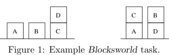
The main idea behind the work discussed in this paper is to extend those previous ideas on orders by not only ordering the (top-level) goals, but also the sub-goals that will necessarily arise during planning, i.e., by also taking into account what we call the landmarks. The key feature of a landmark is that it must be true at some point on any solution path to the given planning task. Consider theBlocksworldtask shown in Figure 1, which will be our illustrative example throughout the paper.

A C D B D C B A

initial state goal

Figure 1: Example Blocksworld task.

For the reader who is weary of seeing toy examples like the one in Figure 1 in the literature, we remark that our techniques arenotprimarily motivated by this example. Our techniques are useful in much more complex situations. We use the depicted toy example only for easy demonstration of some of the important points. In the example, clear(C) is a landmark because it will need to be achieved in any solution plan. Immediately stacking B on D from the initial state will achieve one of the top level goals of the task but it will result in wasted effort ifclear(C) is not achieved first. To orderclear(C)beforeon(B D) is, however,notreasonable in terms of Koehler and Hoffmann’s definition. First,clear(C)is not a top level goal so it is not considered by Koehler and Hoffmann’s techniques. Second, there are states where B is on D and from whichclear(C) can be achieved without unstacking B from D again (compare the definition of reasonable orders given above). But reaching such a state requires unstacking D from C, and thus achievingclear(C), in the first place. This, together with the fact that clear(C)must be made true at some point, makes it sensible to order clear(C) beforeon(B D).

We propose a natural extension of Koehler and Hoffmann’s definitions to the more general case of landmarks (trivially, all top level goals are landmarks, too). We also revise parts of the original definition to better capture the intuitive meaning of a goal ordering. The extended and revised definitions capture, in particular, situations of the kind demonstrated withclear(C)≤on(B D)in the toy example above. We also introduce a new kind of ordering that often occurs between landmarks: A can be ordered beforeB if all valid solution plans make A true before they make B true. We call such orders necessary. Typically, a fact isa landmark because it is necessarily ordered before some other landmark. For example, clear(C) is necessarily ordered before holding(C), and holding(C) is necessarily ordered before the top level goal on(C A), in the aboveBlocksworld example.

Deciding if a fact is a landmark, and deciding about our ordering relations, is PSPACE-complete. We describe pre-processing techniques that extract landmarks, and that approx-imate necessary orders between them. We introduce sufficient criteria for the existence of reasonable orders between landmarks. The criteria are based on necessary orders, and inconsistencies between facts.1 Using an inconsistency approximation technique from the

literature, we approximate reasonable orders based on our sufficient criteria. After these pre-processes have terminated, what we get is a directed graph where the nodes are the found landmarks, and the edges are the orders found between them. We call this graph the landmark generation graph, short LGG. This graph may contain cycles because for some of our orders there is no guarantee that there is a plan, or even an action sequence, that obeys them.2 Our method for structuring the search for a plan can not handle cycles in the LGG, so we remove cycles by removing edges incident upon them. We end up with a polytree structure.3

Once turned into a polytree, the LGG can be used to decompose the planning task into small chunks. We propose a method that does not depend on any particular planning framework. The landmarks provide a search control loop that can be used around any base planner that is capable of dealing with STRIPS input. The search control does not preserve optimality so there is not much point in using it around optimal planners such as Graphplan (Blum & Furst, 1997) and its relatives. Optimal planners are generally outperformed by sub-optimal planners anyway. It does make sense, however, to use the control in order to further improve the runtime performance of sub-optimal approaches to planning. To demonstrate this, we used the technique for control of two versions of FF (Hoffmann, 2000; Hoffmann & Nebel, 2001), and for control of LPG (Gerevini, Saetti, & Serina, 2003). We evaluated these planners across a range of 8 domains. We consistently obtain, sometimes dramatic, runtime improvements for the FF versions. We obtain runtime improvements for LPG in around half of the domains. The runtime improvement is, for all the planners, usually bought at the cost of slightly longer plans. But there are also some cases where the plans become shorter when using landmarks control.

The paper is organised as follows. Section 2 gives the basic notations. Section 3 defines what landmarks are, and in what relations between them we are interested. Exact compu-tation of the relevant pieces of information is shown to be PSPACE-complete. Section 4 explains our approximation techniques, and Section 5 explains how we use landmarks to structure the search of an arbitrary base planner. Section 6 provides our empirical results in a range of domains. Section 7 closes the paper with a discussion of related work, of our con-tributions, and of future work. Most proofs are moved into Appendix A, and replaced in the text by proof sketches, to improve readability. Appendix B provides runtime distribution graphs as supplementary material to the tables provided in Section 6. Appendix C discusses some details regarding our experimental implementation of landmarks control around LPG. 2. Notations

We consider sequential planning in the propositional STRIPS (Fikes & Nilsson, 1971) frame-work. In the following, all sets are assumed to be finite. A state s is a set of logical facts (atoms). An action ais a triple a= (pre(a), add(a), del(a)) where pre(a) are the action’s preconditions, add(a) is its add list, and del(a) is its delete list, each a set of facts. The

2. Also, none of our ordering relations is transitive. We stick to the word “order” only because it is the most intuitive word for constraints on the relative points in time at which planning facts can or should be achieved.

3. Removing edges incident on cycles might, of course, throw away useful ordering information. Coming up with other methods to treat cycles, or with methods that can exploit the information contained in them, is an open research topic.

result of applying (the action sequence consisting of) a single action ato a states is:

Result(s,hai) = (

(s∪add(a))\del(a) pre(a)⊆s

undefined otherwise

The result of applying a sequence of more than one action to a state is recursively defined as

Result(s,ha1, . . . , ani) =Result(Result(s,ha1, . . . , an−1i),hani). Applying an empty action sequence changes nothing, i.e.,Result(s,hi) =s. A planningtask(A, I, G) is a triple where

A is a set of actions, and I (the initial state) and G (the goals) are sets of facts (we use the word “task” rather than “problem” in order to avoid confusion with the complexity-theoretic notion of decision problems). A plan, orsolution, for a task (A, I, G) is an action sequence P ∈A∗ such that G⊆Result(I, P).

3. Ordered Landmarks: What They Are

In this section we introduce our framework. We define what landmarks are, and in what relations between them we are interested. We show that all the corresponding decision problems are PSPACE-complete. Section 3.1 introduces landmarks and necessary orders, Section 3.2 introduces reasonable orders, and Section 3.3 introduces obedient reasonable orders (orders that are reasonable if one has already committed to obey a given a-priori set of reasonable ordering constraints).

3.1 Landmarks, and Necessary Orders

Landmarks are facts that must be true at some point during the execution of any solution plan.

Definition 1 Given a planning task (A, I, G). A fact L is a landmark if for all P = ha1, . . . , ani ∈A∗, G⊆Result(I, P) :L∈Result(I,ha1, . . . , aii) for some 0≤i≤n.

Note that in an unsolvable taskallfacts are landmarks (by universal quantification over the empty set of solution plans in the above definition). The definition thus only makes sense if the task at hand is solvable. Indeed, while our landmark techniques can help a planning algorithm to find a solution plan faster (as we will see later), they are not useful for proving unsolvability. The reasonable orders we will introduce are based on heuristic notions that make sense intuitively, but that are not mandatory in the sense that every solution plan obeys them, or even in the sense that there exists a solution plan that obeys them. Details on this topic are given with the individual concepts below. We remark that we make these observations only to clarify the meaning of our definitions. Given the way we use the landmarks information for planning, for our purposes it is not essential if or if not an ordering constraint is mandatory. Our search control loop only suggests to the planner what might be good to achieve next, it does not force the planner to do so (see Section 5). Initial and goal facts are trivially landmarks: set i to 0 respectively n in Definition 1. In general, it is PSPACE-complete to decide whether a fact is a landmark or not.

Theorem 1 LetLANDMARK_{denote the following problem: given a planning task(A, I, G),} and a fact L; is L a landmark?

Proof Sketch: PSPACE-hardness follows by a straightforward reduction of the comple-ment of PLANSAT– the decision problem of whether there exists a solution plan to a given arbitrary STRIPS task (Bylander, 1994) – to the problem of deciding LANDMARK_.

PSPACE-membership follows vice versa. 2

Full proofs are in Appendix A. One of the most elementary ordering relations between a pairLand L′ of landmarks is the following. In any action sequence that makesL′ true in some state, L is true in the immediate preceding state. Typically, a fact L is a landmark because it is ordered in this way before some other landmark L′_{. The reason is typically}

thatLis a necessary prerequisite – a shared precondition – for achievingL′. We will exploit this for our approximation techniques in Section 4.

Definition 2 Given a planning task (A, I, G), and two factsLandL′. There is anecessary order between L and L′, written L→nL′, ifL′ 6∈I, and for all P =ha1, . . . , ani ∈ A∗: if

L′ _{∈Result(I,ha}

1, . . . , ani) then L∈Result(I,ha1, . . . , an−1i).

The definition allows for arbitrary facts, but the case that we will be interested in is the case where L and L′ _{are landmarks. Note that if L}′ _{∈Result(I,ha}

1, . . . , ani) then n≥ 1 as L′ 6∈I. The intention behind a necessary order L→n L′ is that one must have L true before one can have L′ true. So it does not make sense to allow such orders for initial facts

L′_{. It is important thatLis postulated to be truedirectlybeforeL}′ _{– this way, if two facts}

L and L′′ are necessarily ordered before the same factL′, one can conclude that Land L′′

must be truetogetherat some point. We make use of this observation in our approximation of reasonable orders (see Section 4.2).

We denote necessary orders, and all the other ordering relations we will introduce, as directed graph edges “→” rather than with the more usual “<” symbol. We do this to avoid confusion about the meaning of our relations. As said earlier, none of the ordering relations we introduce is transitive. (Note that →n would be transitive ifL was only postulated to hold sometime beforeL′, not directly before it.)

Necessary orders are mandatory. We say that an action sequence ha1, . . . , ani obeys an order L → L′ _{if the sequence makes L true the first time before it makes L}′ _{true the first}

time. Precisely, ha1, . . . , ani obeys L → L′ if either L ∈ I, or min{i | L ∈ add(ai)} <

min{i | L′ _{∈ add(a}

i)} where the minimum over an empty set is ∞. That is, either L is true initially, or L′ _{is not added at all, or L is added before L}′_{. By definition, any action}

sequence obeys necessary orders. So one does not lose solutions if one forces a planner to obey necessary orders, i.e. if one disallows plans violating the orders. (We reiterate that this is a purely theoretical observation; as said above, our search control does not enforce the found ordering constraints.)

Theorem 2 Let NECESSARY-ORD _{denote the following problem: given a planning task} (A, I, G), and two facts L and L′; does L→nL′ hold?

Deciding NECESSARY-ORD _{is PSPACE-complete.}

Proof Sketch: PSPACE-hardness follows by reducing the complement of PLANSAT to NECESSARY-ORD_{. PSPACE-membership follows with a non-deterministic algorithm that} guesses action sequences and checks if there is a counter example to the ordering. 2

Another interesting relation aregreedy necessary orders, a slightly weaker version of the necessary orders above. We postulate not thatL is true prior toL′ in all action sequences, but only in those action sequences where L′ is achieved for the first time. These are the orders that we actually approximate and use in our implementation (see Section 4). Definition 3 Given a planning task (A, I, G), and two facts L and L′. There is a greedy necessary orderbetweenLandL′, writtenL→gnL′, ifL′ 6∈I, and for allP =ha1, . . . , ani ∈

A∗_{: if L}′ _{∈ Result(I,ha}

1, . . . , ani) and L′ 6∈ Result(I,ha1, . . . , aii) for 0 ≤ i < n, then

L∈Result(I,ha1, . . . , an−1i).

Like above with the necessary orders, the action sequence achieving L′ must contain at least one step as L′ _{6∈I. Obviously, →}

n is stronger than →gn, that is, with L →n L′ for two facts L and L′, L→gn L′ follows. Greedy necessary orders are still mandatory in the sense that every action sequence obeys them.

The definition of greedy necessary orders captures the fact that, really, what we are interested in is what happens when we directly achieveL′from the initial state, rather than in some remote part of the state space. The consideration of these more remote parts of the state space, which is inherent in the definition of the non-greedy necessary orders, can make us lose useful information. Consider the Blocksworld example in Figure 1. There is a greedy necessary order between clear(D) and clear(C),clear(D) →gn clear(C), but not a necessary order, clear(D)6→nclear(C). If we makeclear(C) true the first time in an action sequence from the initial state, then the action achievingclear(C)will always beunstack(D C), which requires clear(D) to be true. On the other hand, there can of course be action sequences which achieve clear(C) by different actions (unstack(A C), for example). But reaching a state where clear(C) can be achieved by such an action involves unstacking D from C, and thus achievingclear(C), in the first place. We will see later (Section 4.2) that the orderclear(D)→gn clear(C)can be used to make the important inference thatclear(C) is reasonably ordered beforeon(B D).

More generally, the definition of greedy necessary orders is made from the perspective that we are interested in ordering the first occurence of the facts L in our desired solution plan. All definitions and algorithms in the rest of this paper are designed from this same perspective. Since a fact might (have to) be made true several times in a solution plan, one could just as well focus on ordering the fact’s last occurence, or any occurence, or several occurences of it. We chose to focus on the first occurences of facts mainly in order to keep things simple. It seems very hard to say anything useful a priori about exactly how often and when some fact will need to become true in a plan. The “greedy assumption” that our approach thus makes is that all the landmarks need to be achieved only once, and that it is best to achieve them as early as possible. Of course this assumption is not always justified, and may lead to difficulties, such as e.g. cycles in the generated LGG (see also Sections 4.4 and 6.8). Generalising our approach to take account of several occurences of the same fact is an open research topic.

Theorem 3 Let GREEDY-NECESSARY-ORD _{denote the following problem: given a} plan-ning task (A, I, G), and two facts L andL′_{; does L→}

gnL′ hold?

Proof Sketch: By a minor modification of the proof to Theorem 2. 2

3.2 Reasonable Orders

Reasonable orders were first introduced by Koehler and Hoffmann (2000), for top level goals. We extend their definition, in a slightly revised way, to landmarks.

Let us first reiterate what the idea of reasonable orders was originally. The idea in-troduced by Koehler and Hoffmann is this. If the planner is in a state s where one goal

L′ has just been achieved, but another goal L is still false, and L′ must be destroyed in order to achieveL, then it might have been better to achieve Lfirst: to get to a goal state from s, the planner will have to delete and re-achieve L′_{. If the same situation arises inall}

statesswhereL′has just been achieved butLis false, then it seems reasonable to generally introduce an ordering constraintL→L′, indicating that L should be achieved prior toL′. The classical example for two facts with a reasonable ordering constraint areonrelations inBlocksworld, whereon(B, C)is reasonably ordered beforeon(A, B)whenever the goal is to have both facts true in the goal state. Obviously, if one achieves on(A, B)first then one has to unstack A again in order to achieveon(B, C).

Think about an unmodified application of Koehler and Hoffmann’s definition to the case of landmarks. Consider a state swhere we have a landmarkL′, but not another landmark

L, and achieving Linvolves deleting L′_{. Does it matter? It might be that we do not need}

to achieve L from s anyway. It might also be that we do not need L′ anymore once we have achieved L. In both cases, there is no need to delete and re-achieve L′, and it does not appear reasonable to introduce the constraint L → L′_{. The question is, under which}

circumstances is it reasonable? The answer is given by the two mentioned counter-examples. The situation matters if 1. we need to achieveLfroms, and 2. we must re-achieve L′ again afterwards. Both conditions are trivially fulfilled when L and L′ are top level goals. Our definition below makes sure they hold for the landmarksL andL′ _{in question.}

We say that there is a reasonable ordering constraint between two landmarksL and L′

if, starting from any state where L′ was achieved beforeL: L′ must be true at some point later than the achievement ofL; and one must deleteL′ _{on the way toL. Formally, we first}

define the “set of states where L′ was achieved before L”, then we define what it means that “L′ must be true at some point later than the achievement ofL”, then based on that we define what reasonable orders are.

Definition 4 Given a planning task (A, I, G), and two factsL and L′.

1. By S₍L′_,¬L), we denote the set of statesssuch that there existsP =ha₁, . . . , ani ∈A∗,

s=Result(I, P), L′ ∈add(an), andL6∈Result(I,ha1, . . . , aii) for 0≤i≤n.

2. L′ is in the aftermath of L if, for all states s ∈ S(L′_,¬L), and all solution plans P = ha1, . . . , ani ∈ A∗ from s, G ⊆Result(s, P), there are 1 ≤i≤ j ≤n such that

L∈Result(s,ha1, . . . , aii) and L′ ∈Result(s,ha1, . . . , aji).

3. There is a reasonable order between L and L′_{, written L →}

r L′, if L′ is in the

aftermath of L, and

Let us explain this definition, and how it differs from Koehler and Hoffmann’s original one.

1. S₍L′,¬L)contains the states whereL′was just added, butLwas not true yet. These are the states we consider: we are interested to know if, from every states∈S(L′_,¬L), we will have to delete and re-achieve L′. In Koehler and Hoffmann’s original definition,

S₍L′,¬L) contained more states, namely all those states swhereL′ was just added but L 6∈ s. This definition allowed cases where L was achieved already but was deleted again. Our revised definition captures better the intuition that we want to consider all states whereL′ _{was achievedbeforeL. The revised definition also makes sure that,}

for a landmarkL, any solution plan starting froms∈S(L′_,¬L)must achieveLat some point.

2. The definition of the aftermath relation just says that, in a solution plan starting froms∈S₍L′_,¬L),L′ must be true simultaneously withL, or at some later time point. Koehler and Hoffmann didn’t need such a definition since this condition is trivially fulfilled for top level goals.

3. The definition of L →r L′ then says that, from every s ∈ S(L′_,¬L), every action sequence achieving L deletes L′ at some point. With the additional postulation that

L′ _{is in the aftermath of L, this implies that from every s ∈ S}

(L′_,¬L) one needs to delete and re-achieve L′. Koehler and Hoffmann’s definition here is identical except that they do not need to postulate the aftermath relation.

Because in their definitionS₍L′,¬L) contains more states, and top level goals are trivially in the aftermath of each other, Koehler and Hoffmann’s→r definition is stronger than ours, i.e. L→rL′ in the Koehler and Hoffmann sense impliesL→rL′ as defined above (we give an example below where our, but not the Koehler and Hoffmann L→rL′ relation holds).4 It is important to note that reasonable orders are not mandatory. An order L →r L′ only says that, if we achieve L′ _{before L, we will need to delete and re-achieve L}′_{. This}

might mean that achieving L′ before L is wasted effort. But there are cases where, in the process of achieving some landmarkL, one has no other choice but to achieve, delete, and re-achieve a landmarkL′_{. In the Towers of Hanoi domain, for example, this is the case for}

nearly all pairs of top level goals – namely, for all those pairs of goals that say that (L′) disc i must be located on disc i+ 1, and (L) disc i+ 1 must be located on disc i+ 2. In such a situation, forcing a planner to obey the order L→r L′ cuts out all solution paths. One can also easily construct cases where L →r L′ and L′ →r L hold for goals L and L′ (that can not be achieved simultaneously). Consider the following example. There are the

4. Note that an orderL→rL′ intends to tell us that we should not achieveL′ beforeL. This leaves open the option to achieveLandL′_{simultaneously. In that sense, our definition (given above in Section 3.1)}

of what it means to obey an orderL→L′_{, namely to addLstrictly before L}′_{, is a bit too restrictive.}

In our experience, the restriction is irrelevant in practice. In none of the many benchmarks we tried did we observe facts that were reasonably ordered (ordered at all, in fact) relative to each other and that could be achieved with the same action – remember that we consider the sequential planning setting. We remark that one can easily adapt our framework to take account of simultaneous achievement ofL

andL′_{. No changes are needed except in the approximation of obedient reasonable orders, which would}

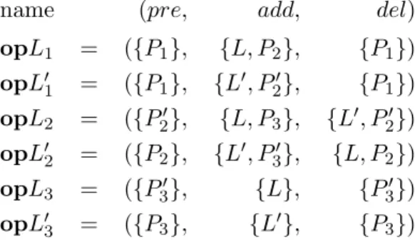
seven facts L, L′,P1,P2,P2′,P3, and P3′. Initially onlyP1 is true, and the goal is to have L andL′. The actions are:

name (pre, add, del)

opL1 = ({P1}, {L, P2}, {P1}) opL′₁ = ({P1}, {L′, P₂′}, {P1}) opL2 = ({P2′}, {L, P3}, {L′, P2′}) opL′₂ = ({P2}, {L′, P₃′}, {L, P2}) opL3 = ({P3′}, {L}, {P3′}) opL′ 3 = ({P3}, {L′}, {P3})

Figure 2 shows the state space of the example. There are exactly two solution paths, h opL1,opL′2,opL3 i and h opL′1,opL2,opL′3 i. The first of these paths achieves, deletes, and re-achieves L, the second one does the same with L′. S₍L′_,¬L) contains the single state that results from applyingopL′

1to the initial state. From that state, one has to applyopL2 in order to achieve L, deletingL′, soL→r L′ holds. Similarly, it can be seen thatL′ →rL holds. Note that either solution path disobeys one of the two reasonable orders.

P’ { L, P }₃ { L’,P’ }₃ { L, L’ } opL 3 opL’ opL’₃ opL 1 2 { P₁} 1 opL’ } } 2 opL₂ { L, P₂ { L’,

Figure 2: State space of the example.

We reiterate that the above are purely theoretical observations made to clarify the mean-ing of our definitions. Our search control does not enforce the found ordermean-ing constraints, it only suggests them to the planner.

While reasonable orders L →r L′ are not mandatory, they can help to reduce search effort in those cases where achievingL′_{beforeLdoesimply wasted effort. OurBlocksworld}

example from Figure 1 constitutes such a case. In the example, it makes no sense to stack B onto D while D is still located on C, because C has to end up on top of A. By Definition 4, clear(C) →r on(B D) holds: S(on(BD),¬clear(C)) contains only states where B has been stacked onto D, but D is still on top of C. From these states, one must delete on(B D) in order to achieve clear(C). Further, on(B D) is a top-level goal so it is in the aftermath ofclear(C), and clear(C) →r on(B D) follows. The order does not hold in terms of Koehler and Hoffmann’s definition, because there the S(on(BD),¬clear(C)) state set also contains states whereDwas already removed fromC.

Like the previous decision problems, those related to the aftermath relation and to reasonable orders are PSPACE-complete.

Theorem 4 LetAFTERMATH_{denote the following problem: given a planning task(A, I, G),} and two facts L and L′; is L′ in the aftermath of L?

Proof Sketch: PSPACE-hardness follows by reducing the complement of PLANSAT to AFTERMATH_{. PSPACE-membership follows by a non-deterministic algorithm that guesses}

counter examples. 2

Theorem 5 Let REASONABLE-ORD _{denote the following problem: given a planning task} (A, I, G), and two facts Land L′ _{such that L}′ _{is in the aftermath ofL; doesL→}

r L′ hold?

Deciding REASONABLE-ORD _{is PSPACE-complete.}

Proof Sketch: PSPACE-hardness follows by reducing the complement of PLANSAT to REASONABLE-ORD_{, with the same construction as used by Koehler and Hoffmann (2000)} for the original definition of reasonable orders. PSPACE-membership follows by a non-deterministic algorithm that guesses counter examples. 2

3.3 Obedient Reasonable Orders

Say we already have a set O of reasonable ordering constraints L→r L′. The question we focus on in the section at hand is, if a planner commits to obey all the constraints inO, do other reasonable orders arise? The answer is, yes, there might.

Consider the following situation. Say we got landmarks L and L′, such that we must delete L′ in order to achieve L. Also, there is a third landmark L′′ such that L′ →n L′′ and L →r L′′. Now, if the order L → L′′ was necessary, L →n L′′, then we would have a reasonable order L →r L′: L and L′ would need to be true together immediately prior to the achievement of L′′, so L′ would be in the aftermath of L. However, the ordering constraint L→ L′′ _{is “only” reasonable so there is no guarantee that a solution plan will}

obey it. A plan can choose to achieve L′ before L′′ before L, and thereby avoid deletion and re-achievement of L′. But if we enforce the ordering constraint L →r L′′, disallowing plans that do not obey it, then achieving L′ _{beforeL leads to deletion and re-achievement}

of L′ and is thus not reasonable.

With the above, the idea we pursue now is to define a weaker form of reasonable or-ders, which are obedient in the sense that they only arise if one commits to a given set O

of (previously computed) reasonable ordering constraints. In our experiments, using (an approximation of) such obedient reasonable orders, on top of the reasonable orders them-selves, resulted in significantly better planner performance in a few domains (such as the Blocksworld), and made no difference in the other domains. Summarised, what we do is, we start from the setO of reasonable orders already computed by our approximations, and then insert new orders that are reasonable given one commits to obey the constraints in

O. We do this just once, i.e. we do not compute a fixpoint. The details are in Section 4.3. Right now, we define what obedient reasonable orders are.

The definition of obedient reasonable orders is almost the same as that of reasonable orders. The only difference lies in that we consider only action sequences that are obedient in the sense that they obey all ordering constraints in the given set O. The definition of when an action sequence ha1, . . . , ani obeys an order L → L′ was already given above: if eitherL∈I, ormin{i|L∈add(ai)}< min{i|L′ ∈add(ai)} where the minimum over an empty set is∞.

Definition 5 Given a planning task (A, I, G), a set O of reasonable ordering constraints, and two facts L and L′.

1. By SO

(L′_,¬L), we denote the set of states s such that there exists an obedient action sequence P = ha1, . . . , ani ∈ A∗, with s = Result(I, P), L′ ∈ add(an), and L 6∈

Result(I,ha1, . . . , aii) for 0≤i≤n.

2. L′ _{is in the obedient aftermath ofLif, for all statess∈S}O

(L′_,¬L), and all obedient solu-tion plansP =ha1, . . . , ani ∈A∗,G⊆Result(I, P), wheres=Result(I,ha1, . . . , aki),

there are k ≤ i ≤ j ≤ n such that L ∈ Result(I,ha1, . . . , aii) and L′ ∈ Result(I,

ha1, . . . , aji).

3. There is an obedient reasonable order between L and L′, written L →O

r L′, if and

only ifL′ _{is in the obedient aftermath ofL, and}

∀s∈S₍O_L′_,¬L):∀P ∈A∗ : L∈Result(s, P)⇒ ∃a∈P :L′ ∈del(a)

This definition is very similar to Definition 4 and thus should be self-explanatory, in its formal aspects. The definition of the aftermath relation looks a little more complicated because the solution planP starts from the initial state, not from sas in Definition 4, and reaches swith action ak. This is just a minor technical device to cover the case where, for some of the L1 →r L2 constraints in O, L1 is contained in s already (and thus does not need to be added aftersin order to obeyL1→rL2). Note that, in part 3 of the definition, the action sequencesP achieving L are not required to be obedient. While it would make sense to impose this requirement, our approximation techniques (that will be introduced in Section 4.3) only take account ofO in the computation of the aftermath relation anyway. It is an open question how our other approximation techniques could be made to take account of O.

We remark that the modified definitions do not change the computational complexity of the corresponding decision problems.5 _{As a quick illustration of the new definitions,} reconsider the situation described above. There, L′ is not in the aftermath of L, but in the obedient aftermath ofLbecause all action sequences that obey the constraint L→rL′′ makeL′ _{true at a point simultaneously with or behindL (namely immediately prior toL}′′_,

assuming that there is no action that adds bothL andL′′_{). AsL}′ _{must be deleted in order}

to achieve L, we obtain the ordering L →{rL→rL′′} L′. That is, if the planner obeys the constraint L→rL′′ then it is reasonable to also orderL beforeL′.

Just like the reasonable orders, the obedient reasonable orders are not mandatory. En-forcing an obedient reasonable order can cut out all solution paths. The reason is the same as for the reasonable orders. An order L →O

r L′ only says that, given we want to obey

O, achieving L′ _{before L implies deletion and re-achievement of L}′_{. If this really means}

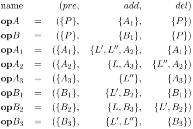
that achieving L′ beforeL is wasted effort, the order tells us nothing about. Consider the following example. There are the ten facts L, L′_{, L}′′_{, P, A}

1, A2, A3, B1, B2, and B3.

5. For the obedient aftermath relation, minor modifications of the proof to Theorem 4 suffice. PSPACE-hardness follows by using the empty set of ordering constraints. PSPACE-membership follows by ex-tending the non-deterministic decision algorithm with flags that check if the ordering constraints are adhered to. Similarly for obedient reasonable orders and the proof to Theorem 5.

Initially only P is true, and the goal is to have L, L′, and L′′. The construction is made so that L→r L′′, andL6→r L′ butL→{L→rL

′′_}

r L′. Enforcing L→{L→rL ′′_}

r L′ renders the task unsolvable. The actions are:

name (pre, add, del)

opA = ({P}, {A1}, {P}) opB = ({P}, {B1}, {P}) opA1 = ({A1}, {L′, L′′, A2}, {A1}) opA2 = ({A2}, {L, A3}, {L′′, A2}) opA3 = ({A3}, {L′′}, {A3}) opB1 = ({B1}, {L′, B2}, {B1}) opB2 = ({B2}, {L, B3}, {L′, B2}) opB3 = ({B3}, {L′, L′′}, {B3})

Figure 3 shows the state space of the example. One has to choose one out of two options. First, one applies opA to the initial state and then proceeds withopA1,opA2, andopA3. Second, one applies opB to the initial state and proceeds with opB1, opB2, and opB3. The first option is the only one whereL′′ becomes true beforeL. One has to deleteL′′with opA2, and re-achieve it with opA3. For this reason, the order L →r L′′ holds. The order

L→rL′ does not hold because if one chooses the first option thenL′ becomes true prior to

L, and is never deleted. However, committing to the order L →r L′′ means excluding the first option. In the second option,L′ _{becomes true beforeL, and must then be deleted and}

re-achieved, so we get the order L→{rL→rL′′} L′. But there is no solution plan that obeys this order because there is no way to make L true before (or, even, simultaneously with)

L′. L’, 2 { opB L, { L’, L’’, A₂} 2 { } opA L, L’, A₃ B }₂ B₃} opA₃ opB₃ { { L, L’, L’’} { P opB opA₁ 1 opB } } 1 1 A opA } B { {

Figure 3: State space of the example.

4. How to Find Ordered Landmarks

We now describe our methods to find landmarks in a given planning task, and to approx-imate their inherent ordering constraints. The result of the process is a directed graph in the obvious way, the landmarks generation graph (LGG). Section 4.1 describes how we find landmarks, and how we approximate greedy necessary orders between them. Section 4.2 gives a sufficient criterion for reasonable orders, based on greedy necessary orders and fact inconsistencies, and describes how we use the criterion for approximating reasonable orders. Section 4.3 adapts this technology to obedient reasonable orders. Section 4.4 describes our

handling of cycles in the LGG, and Section 4.5 describes a preliminary form of “lookahead” orders that we have also implemented and used.

4.1 Finding Landmarks and Approximating Greedy Necessary Orders

We find (a subset of the) landmarks in a planning task, and approximate the greedy neces-sary orders between them, both in one process. The process is split into two parts:

1. Compute an LGG of landmark candidates together with approximated greedy necessary orders between them. This is done with a backchaining pro-cess. The goals form the first landmark candidates. Then, for any candidate L′_{, the}

“earliest” actions that can be used to achieve L′ are considered. Here, “early” is a greedy approximation of reachability from the initial state. The actions are analysed to see if they have shared precondition factsL– facts that must be true before execut-ing any of the actions. These factsLbecome new candidates if they have not already been processed, and the ordersL→gn L′ are introduced. The process is iterated until there are no new candidates. (Due to the greedy selection of actions, L/the order

L→gnL′ is not proved to be a landmark/a greedy necessary order.)

2. Remove from the LGG the candidates (and their incident edges) that can not be proved to be landmarks. This is done by evaluating a sufficient condition on each candidateLin the LGG. The condition ignores all actions that addL, and asks if a relaxed version of the task is still solvable. If not, Lis proved to be a landmark. (Any relaxation can be used in principle; we use the relaxation that ignores delete lists as in McDermott, 1999 and Bonet & Geffner, 2001.)

The next two subsections focus on these two steps in turn.

4.1.1 Landmark Candidates

We give pseudo-code for our approximation algorithm below. As said, we make the algo-rithm greedy by using an approximation of reachability from the initial state. The approx-imation we use is a relaxed planning graph (Hoffmann & Nebel, 2001), short RPG. Let us explain this data structure first. An RPG is built just like a planning graph (Blum & Furst, 1997), except that the delete lists of all actions are ignored; as a result, there are no mutex relations in the graph. The RPG thus is a sequence P0, A0, P1, A1, . . . , Pm−1, Am−1, Pm of proposition sets (layers)Pi and action sets (layers)Ai. P0contains the facts that are true in the initial state, A0 contains those actions whose preconditions are reached (contained) in P0,P1 contains P0 plus the add effects of the actions inA0, and so on. We have Pi ⊆Pi+1 and Ai ⊆ Ai+1 for all i. If the relaxed task (without delete lists) is unsolvable, then the RPG reaches a fixpoint before reaching the goal facts, thereby proving unsolvability. If the relaxed task is solvable, then eventually a layer Pm containing the goal facts will be reached.6

6. Note that the RPG thus decides solvability of the relaxed planning task. Indeed, building an RPG is a variation of the algorithm given by Bylander (1994) to prove that plan existence is polynomial in the absence of delete lists.

An RPG encodes an over-approximation of reachability in the planning task. We define thelevelof a fact/action to be the index of the first proposition/action layer that contains the fact/action. Then, if the level of a fact/action is l, one must apply at leastlparallel action steps from the initial state before the fact becomes true/the action becomes applicable. (The fact/action level corresponds to the “h1” heuristic defined by Haslum & Geffner, 2000.) We use this over-approximation of reachability to insert some greediness into our approximation of “greedy” necessary orders (more below). The approximation process proceeds as shown in Figure 4.

initialise the LGG to (G,∅), and set C:=G

whileC6=∅ do

setC′ _:=∅

forallL′_{∈C, level(L}′_{)6= 0do}

letAbe the set of all actionsasuch thatL′_{∈add(a), andlevel(a) =level(L}′_{)−1 (∗)} forall facts Lsuch that∀a∈A:L∈pre(a)do

ifLis not yet a node in the LGG, setC′ _:=C′_{∪ {L}}

ifLis not yet a node in the LGG, then insert that node

ifL→gnL′ is not yet an edge in the LGG, then insert that edge

endfor endfor

setC :=C′ endwhile

Figure 4: Landmark candidate generation.

The set of landmark candidates is initialised to comprise the goal facts. Each iteration of the while-loop processes all “open” candidatesL′ _{– those L}′ _{inC. Candidates L}′ _with

level 0, i.e., initial facts, are not used to produce greedy necessary orders and new landmark candidates, because after all such L′ are already true. For the other open candidates L′, the set A comprises all those actions at the level below L′ _{that can be used to achieve}

L′. Note that these are the earliest possible achievers of L′ in the RPG, or else the level of L′ would be lower. We take as the new landmark candidates those facts L that every action inArequires as a precondition, and update the LGG and the set of open candidates accordingly. Independently of the (∗) step, the algorithm terminates because there are only finitely many facts. Because we use the RPG level test in step (∗), the levels of the new candidates Lare strictly lower than the level of L′, and the while-loop terminates after at mostm iterations wherem is the index of the topmost proposition layer in the RPG.

If we skipped the test for the RPG level at the point in the algorithm marked (∗), then the new candidatesLwould be proved landmarks, and the generated orders would be proved to be necessary and thus also greedy necessary. Obviously, if allactions that can achieve a landmark L′ require L to be true, then L is a landmark that must be true immediately prior to achieving L′. Restricting the choice of L′ achievers with the RPG level test, the found landmarks and orders may be unsound. Consider the following example, where we want to move from city A to city D on the road map shown in Figure 5, using a standard moveoperator.

A B C D E

Figure 5: An example road map.

The above algorithm will come up with the following LGG:{at(A), at(E), at(D)},{at(A) →gn at(E),at(E) →gn at(D)} – the RPG is only built until the goals are reached the first time, which happens in this example before move(C D) comes in. However, the action sequence hmove(A B), move(B C), move(C D)i achieves at(D) without makingat(E) true. Therefore, at(E) is not really a landmark, and at(E) →gn at(D) is not really a greedy necessary order.

By restricting our choice ofL′ achievers with the RPG level test at step (∗) in Figure 4, as said we intend to insert greediness into our approximation of greedy necessary orders. The generated orders L →gn L′ are only guaranteed to be sound if, in the RPG, the set of earliest achievers of L′ contains all actions that can be used to make L′ true for the first time from the initial state. Of course, it is hard to exactly compute that latter set of actions, and also it is highly non-trivial – if possible at all – to find general conditions on when the earliest achievers in the RPG contain all these actions. In the road map example above, the actions that can achieve at(D) for the first time aremove(C D)andmove(E D), but the only earliest achiever in the RPG is move(E D). This leads to the unsound at(E) →gn at(D) order. In the following example taken from the well-known Logistics domain, the earliest achievers of L′ do contain all actions that can make L′ true for the first time. SayL′ =at(P A)requires packagePto be at the airportAof its origin city, andPis not at this airport initially. The actions that can achieve L′ _{are to unload P from the local truck}

T, or to unload it from any airplane. The only earliest achiever in the RPG is the unload fromT, and indeed that’s the only action that can achieveL′ _{for the first time – in order to}

get the package into an airplane, the package has to arrive at the airport in the first place. Our approximation process correctly generates the new landmark candidatein(P T)as well as the greedy necessary orderin(P T)→gn at(P A). Note that in(P T)6→n at(P A).

We show below in Section 4.1.2 how we re-establish the soundness of the landmark can-didates, removing candidates (and their associated orders) that are not provably landmarks. We did not find a way to provably re-establish the soundness of the generated greedy neces-sary orders, and unsound orders may stay in the LGG, potentially also causing the inference of unsound reasonable/obedient reasonable orders (see the sections below). We did observe such unsoundness in a few domains during our experiments (individual discussions are in Section 6). We remark the following.

1. While unsound approximated L →gn L′ orders are not valid with respect to Defini-tion 3, they still make some sense intuitively. They are generated becauseL is in the preconditions of all actions that are the first ones in the RPG to achieve L′. This means that going toL′ via Lis probably a good option, in terms of distance from the initial state.

2. UnlessLis a landmark for some other reason (than for the unsound orderL→gn L′), landmark verification will remove L, and in particular the order L→gn L′, from the

LGG (see the discussion of the Figure 5 example below in the section about landmark verification).

3. As said before, our search control does not enforce the orders in the LGG, it only suggests them to the planner. So even if there is no plan that obeys an order in the LGG, this does not mean that our search control will make the planner fail.

4. If we were to extract only provably necessary orders, by not using the RPG level test, we would miss the information that lies in those →gn orders that are not→n orders. For these reasons, in particular for the last one, we concentrated on the potentially unsound RPG-based approximation in our experiments. We also ran some comparative tests to the “safe” strategy without the RPG level test, in domains where the RPG produced unsound orders. See the details in Section 6.

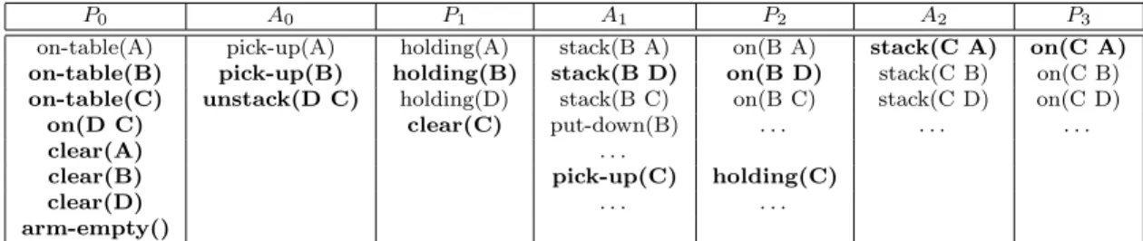
One case where an →gn order, that is not an →n order, contains potentially useful information, is theLogisticsexample given above. Another case is the aforementioned order clear(D)→gn clear(C)in our runningBlocksworldexample from Figure 1. To conclude this subsection, let us have a look at what our approximation algorithm from Figure 4 does in that example. The RPG for the example is summarised in Figure 6.

P0 A0 P1 A1 P2 A2 P3

on-table(A) pick-up(A) holding(A) stack(B A) on(B A) stack(C A) on(C A) on-table(B) pick-up(B) holding(B) stack(B D) on(B D) stack(C B) on(C B)

on-table(C) unstack(D C) holding(D) stack(B C) on(B C) stack(C D) on(C D)

on(D C) clear(C) put-down(B) . . . .

clear(A) . . .

clear(B) pick-up(C) holding(C)

clear(D) . . . .

arm-empty()

Figure 6: Summarised RPG for the illustrative Blocksworld example from Figure 1. As we explained above, the extraction process starts by considering the goals on(C A) andon(B D)as landmark candidates. The RPG level ofon(C A)is 3, the level ofon(B D)is 2. There is only one action with level 2 that achieves on(C A):stack(C A). So, holding(C) (level 2) and clear(A) (level 0) are new candidates. The new LGG is: ({on(C A),on(B D),holding(C),clear(A)},{holding(C) →gn on(C A), clear(A) →gn on(C A)}). Processing

on(B D), we find that its only earliest achiever is stack(B D), and we generate the new candidatesholding(B)(level 1) andclear(D)(level 0) with the respective edges. In the next iteration, holding(C) (level 2) produces the new candidatesclear(C) (level 1), on-table(C) (level 0), and arm-empty() (level 0) by the achiever pick-up(C); and holding(B) (level 1) produces the new candidates on-table(B) (level 0) and clear(B) (level 0) by the achiever pick-up(B). In the third and final iteration of the algorithm, clear(C) (level 1) produces the new candidate on(D C) (level 0) by the achiever unstack(D C). The process ends up with the LGG as shown in Figure 7 (the edges in the depicted graph are all directed from bottom to top). Fact sets of which our LGG suggests that they have to be true together at some point – because they are either top level goals, or →gn ordered before the same

fact – are grouped together in boxes. As said before, this information is important for the approximation of reasonable orders described below.

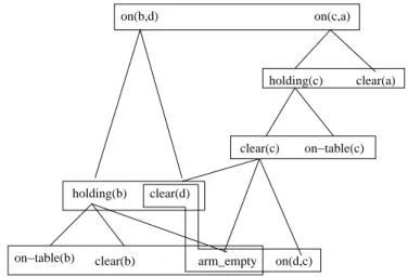
on(c,a) clear(a) on−table(c) clear(c) holding(c) clear(d) holding(b) on(b,d) arm_empty on(d,c) on−table(b) _clear(b)

Figure 7: LGG for the illustrative Blocksworld task, containing the found landmarks and →gn orders.

4.1.2 Landmark Verification

As said before, we verify landmark candidates by evaluating a sufficient condition on them, and throwing away those candidates where the condition fails. The condition we use is the following.

Proposition 1 Given a planning task (A, I, G), and a factL. Define a modified action set AL as follows.

AL:={(pre(a), add(a),∅) |(pre(a), add(a), del(a))∈A, L6∈add(a)}

If (AL, I, G) is unsolvable, then L is a landmark in (A, I, G).

Note that the inverse direction of the proposition does not hold – that is, if L is a landmark in (A, I, G) then (AL, I, G) is not necessarily unsolvable – because ignoring the delete lists simplifies the achievement of the goals. As mentioned earlier, deciding about solvability of planning tasks with empty delete lists can be done in polynomial time by building the RPG. The task is unsolvable iff the RPG can’t reach the goals. So our landmark verification process looks at all landmark candidates in turn. Candidates that are top level goals or initial facts are trivially landmarks, so they need not be verified. For each of the other candidatesL, the RPG corresponding to (AL, I, G) is built, and if that RPG reaches the goals, thenL and its incident edges are removed from the LGG.

Reconsider the road map example depicted in Figure 5. The LGG built will be {at(A), at(E), at(D)},{at(A) →gn at(E), at(E) →gn at(D)}. But at(E) is not really a landmark because the action sequence hmove(A,B), move(B,C), move(C,D)i achieves at(D). When

verifying at(E), we detect this. In the RPG, when ignoring all actions that achieve at(E), move(A,B), move(B,C), and move(C,D) stay in and so the goal remains reachable. Thus at(E) and its edges (in particular, the invalid edgeat(E) →gn at(D)) are removed, yielding the final (trivial) LGT with node set{at(A),at(D)}and empty edge set. Note that, ifat(E) was a landmark for some other reason than reaching D (like, if one had to pick up some object at E), then at(E) would not be removed by landmark verification and the invalid order at(E) →gn at(D) would stay in.

In the Blocksworld example from Figure 1, landmark verification does not remove any candidates, and the LGG remains unchanged as depicted in Figure 7.

4.2 Approximating Reasonable Orders

Our process to approximate reasonable orders starts from the LGG as computed by the methods described above, and enriches the LGG with new edges corresponding to the approximated reasonable orders. The process has two main aspects:

1. We approximate the aftermath relation based on the LGG. This is done by evaluating a sufficient condition that covers certain cases when greedy necessary orders imply the aftermath relation.

2. We combine the aftermath relation with interference information to ap-proximate reasonable orders. For each pair of landmarksL′ _{andLsuch thatL}′ _is

in the aftermath ofLaccording to the previous approximations, a sufficient condition is evaluated. The condition covers certain cases whenL interferes with L′, i.e., when achieving L (from a state in S₍L′_,¬L)) involves deleting L′. If the condition holds, a reasonable order L→rL′ is introduced.

The next two subsections focus on these two aspects in turn. In our implementation, the computation of the aftermath relation is interleaved with its combination with interfer-ence information. Pseudo-code for the overall algorithm is given in the second subsection, Figure 8.

4.2.1 Aftermath Relation

The sufficient condition that we use to approximate the aftermath relation is the following. Lemma 1 Given a planning task (A, I, G), and two landmarks L and L′. If either

1. L′ ∈G, or

2. there are landmarks L = L1, . . . , Ln+1, n ≥ 1, Ln 6= L′, such that Li →gn Li+1 for 1≤i≤n, and L′ →gn Ln+1,

then L′ is in the aftermath ofL.

Proof Sketch: IfL′ ∈Gthen L′ is trivially in the aftermath of L. Otherwise, under the given circumstances,L′ _andL

n must be true together at some point in any action sequence achieving the goal from a state in S(L′_,¬L), namely directly prior to achievement of Ln+1.

AsL has a path of →gn orders to Ln, it has to be true prior to (or simultaneously with, if

n= 1) L′. 2

Note that this lemma just captures the property we mentioned before, when we can tell from the LGG that several facts must be true together at some point. In the second case of the lemma, these facts are L′ and Ln. L′ and Ln are both ordered →gn before Ln+1 and so must be true together before achieving that fact. The first case of the lemma can be understood this way as implicitly assuming Ln as some other top-level goal that L has a path of →gn orders to. (In our implementation, L must have such a path in the LGG or it would not have been generated as a landmark candidate.) IfL′ and Ln must be true together, and we additionally know thatLmust be true sometime beforeLn, then we know thatL′ is in the aftermath of L.7

The most straightforward idea to make use of Lemma 1 would be to simply enumerate all pairs of nodes (landmarks) in the LGG, and evaluate the lemma, collecting the pairs

L and L′ _{of landmarks where the lemma condition holds. While this would probably not}

be prohibitively runtime-costly, one can do better by having a closer look at the lemma condition. Consider each node L′ in the LGG in turn. If L′ is a top level goal, then L′

is in the aftermath of all other nodes L. If L′ _{is not a top level goal, then consider all}

nodesLn6=L′ such that L′ and Ln both have a →gn order before some other node Ln+1. The nodes Lin the LGG that have an (possibly empty) outgoing →gn path to such an Ln are exactly those for which L′ _{is in the aftermath of L according to Lemma 1. As said,}

pseudo-code for our overall approximation of reasonable orders is given below in Figure 8. Note that the inputs to Lemma 1 are→gnorders, while in practice we evaluate the lemma on the edges in the LGG as generated by the processes described above in Section 4.1. As we discussed above, the edges in the LGG may be unsound, i.e. they do not provably correspond to →gn orders. In effect, neither can we guarantee that our approximation to the aftermath relation is sound.

4.2.2 Reasonable Orders

We approximate reasonable orders by considering all pairs L and L′ where L′ is in the aftermath of L according to the above approximation. We test if L interferes with L′

according to the definition directly below. If the test succeeds, we introduce the order

L→rL′.

Definition 6 Given a planning task (A, I, G), and two facts L and L′_{. L interferes with}

L′ if one of the following conditions holds: 1. L and L′ are inconsistent;

2. there is a fact x∈T

a∈A,L∈add(a)add(a), x6=L, such that x is inconsistent with L′; 3. L′ _∈T

a∈A,L∈add(a)del(a);

4. or there is a landmark x inconsistent with L′ such that x→gnL. 7. In theory, one could also allowL′ _=L

n 6=Lin Lemma 1. In this case,L has a path of→gn orders to

L′_{, which trivially implies thatL}′ _{is in the aftermath ofL. But in fact, it is then impossible to achieve} L′_{beforeLso an orderL→}

As said before, our (standard) definition of inconsistency is that facts x and y are inconsistent in a planning task if there is no reachable state in the task that contains both

x and y.8 Note that the conditions 1 to 4 of Definition 6, while they may look closely related at first sight (and presumably are related in many practical examples), indeed cover different cases of when achieving L involves deletingL′. More formally expressed, for each conditionithere are cases whereiholds but no conditionj6=iholds. For example, consider condition 2. In the following example, there is a reasonable orderL→rL′, andLinterferes with L′ due to condition 2 only. There are the six facts L,L′,x, P1, P2, and P′. Initially only P′ is true, and the goal is to have Land L′. The actions are:

name (pre, add, del)

opL′ _{= ({P}′_{}, {L}′_{}, {x})}

opP1 = ({P′}, {P1}, {L′, P′}) opP2 = ({P′}, {P2}, {L′, P′}) opL1 = ({P1}, {L, x, P′}, {P1}) opL2 = ({P2}, {L, x, P′}, {P2})

In this example, the only action sequences that are possible are of the form (opL′ k opP1 ◦ opL1 k opP2 ◦ opL2)∗, in BNF-style notation. In effect, L →r L′ because if we achieve L′ first, we have to apply one ofopP1 and opP2, which both deleteL′. Condition 2 holds: x is inconsistent withL′ and added by both opL1 and opL2. As for condition 1, L and L′ _{are not inconsistent because one can apply opL}′ _{after, e.g., opL}

1. Condition 3 is obviously not fulfilled, and condition 4 is not fulfilled because there are two options to achieve Lso no fact has a →gn order beforeL.

Interference together with the aftermath relation implies reasonable orders between landmarks.

Theorem 6 Given a planning task(A, I, G), and two landmarks L and L′_{. IfL interferes}

withL′, and either 1. L′ ∈G, or

2. there are landmarks L = L1, . . . , Ln+1, n ≥ 1, Ln 6= L′, such that Li →gn Li+1 for 1≤i≤n, and L′ →gn Ln+1,

then there is a reasonable order between L andL′, L→rL′.

Proof Sketch: By Lemma 1,L′ _{is in the aftermath of L. Let us look at the four possible}

reasons for interference. If L is inconsistent with L′ _{then obviously achieving L involves}

deleting L′. If all actions that achieveL add a fact that is inconsistent with L′, the same argument applies. The case where all actions that achieve L delete L′ _{is obvious. As for}

8. Deciding about inconsistency is obviously PSPACE-hard. Just imagine a task where we insert one of the facts into the initial state, and the other fact such that it can only be made true once the original goal has been achieved. We approximate inconsistency with a sound but incomplete technique developed by Maria Fox and Derek Long (1998), see below.

the last case, say we are in a state s∈S(L′_,¬L). Then x is not in s(because L′ is). Due to x→gn L,x must be achieved directly prior toL, and thus L′ will be deleted. 2 Overall, our method for approximating reasonable orders based on the LGG works as specified in Figure 8. With what was said above, the algorithm should be self-explanatory except for the interference tests. When doing these tests, we need information about fact inconsistencies, and, for condition 4 of Definition 6, about→gn orders. Our approximation to the latter pieces of information are, as before, the (approximate)→gnedges in the LGG. Our approximation to the former piece of information is a technique from the literature (Fox & Long, 1998), the TIM API. This provides a functionTIMinconsistent(x,y) that, for facts x and y, returns TRUE only if x and y are inconsistent. The function is incomplete, i.e., it can return FALSE even if x and y are inconsistent.

forall nodesL′ _{in the LGGdo}

ifL′_∈Gthen

forall nodesL6=L′ _{in the LGGdo}

ifL interferes withL′_{, then insert the edgeL→rL}′ _{into the LGG} endfor

else

forall nodesLn6=L′ in the LGG

s.t. there are a nodeLn+1and edgesL′→gnLn+1,Ln→gnLn+1 in the LGGdo forall nodesLin the LGG

s.t. Lhas an (possibly empty) outgoing path of →gnedges toLndo ifL interferes withL′_{, then insert the edgeL→rL}′ _{into the LGG} endfor

endfor endif endfor

Figure 8: Approximating reasonable orders based on the LGG.

Note that the algorithm from Figure 8 might generate ordersL→r L′ in cases whereL already has a path of→gn edges toL′. As noted earlier, in this caseL′ can not be achieved beforeL so the orderL→r L′ is meaningless. One could avoid such meaningless orders by an additional check to see, for every generated pairLandL′, ifLhas an outgoing→gnpath to L′. We do this in our implementation only for the easy-to-check special cases where the length of the →gn path fromL to L′ is 1 or 2. Note that the superfluous→r orders don’t hurt anyway; in fact they don’t change our search process (Section 5.1) at all. The only purpose of our special case test is to avoid some unnecessary evaluations of Definition 6.

Because the inputs to our approximation algorithm are →gn edges in the LGG, and as discussed before these edges are not provably sound, the resulting →r orders are not provably sound (which they otherwise would be by Theorem 6).

Let us finish off our running Blocksworld example, by showing how the order clear(C) →r on(B D), our motivating example from the introduction, is found. Have a look at the LGG in Figure 7. Say the process depicted in Figure 8 considers, in its outermostfor-loop, the LGG node L′ = on(B D). L′ is a top level goal so all other nodes L in the LGG, in particularL=clear(C), are considered in the innerfor-loop. Now,clear(C) interferes with

on(B D) because of condition 4 in Definition 6: clear(D)is inconsistent withon(B D), and has an edgeclear(D) →gn clear(C)in the LGG. Consequently the order clear(C) →r on(B

D)is inferred and introduced into the LGG. Note that, to make this inference, we need the edgeclear(D) →gn clear(C) which isnot a→n order.

4.3 Approximating Obedient Reasonable Orders

The process that approximates obedient reasonable orders starts from the LGG already containing the approximated reasonable orders, and inserts new orders that are reasonable given one commits to the →r orders already present in the LGG. The technology is very similar to the technology we use to approximate reasonable orders. Largely, we do the same thing as before and just treat the→redges as if they were additional→gn edges. Formally, the difference lies in the sufficient criterion for the, now obedient, aftermath relation. Lemma 2 Given a planning task (A, I, G), a set O of reasonable ordering constraints, and two landmarks L and L′. If either

1. L′ ∈G, or

2. there are landmarks L = L1, . . . , Ln+1, n ≥ 1, Ln 6= L′, such that Li →gn Li+1 or Li →rLi+1∈O for 1≤i≤n, and L′ →gnLn+1,

then L′ _{is in the obedient aftermath ofL.}

Proof Sketch: By a simple modification of the proof to Lemma 1. The first case is obvious, in the second case L′ must be true one step beforeLn+1 becomes true, andL must be true

sometime before that. 2

Note that the proved property does not hold if there is only a reasonable order between

L′ _{and L}

n+1, L′ →r Ln+1 instead of L′ →gn Ln+1, even if we have committed to obey L′ →r Ln+1. It is essential thatL′ must be truedirectly beforeLn+1.9

The parts of our technology that do not depend on the aftermath relation remain un-changed. Interference is defined exactly as before. Together with the obedient aftermath relation, it implies obedient reasonable orders between landmarks.

Theorem 7 Given a planning task (A, I, G), a set O of reasonable ordering constraints, and two landmarks L and L′_{. If L interferes with L}′_{, and either}

1. L′ _{∈G, or}

2. there are landmarks L = L1, . . . , Ln+1, n ≥ 1, Ln 6= L′, such that Li →gn Li+1 or Li →rLi+1∈O for 1≤i≤n, and L′ →gnLn+1,

then there is an obedient reasonable order between L and L′, L→O r L′.

9. If obeying an oderL1→rL2 is defined to include the case whereL1 andL2 are achieved simultaneously, the lemma does not hold. The facts L1, . . . , Ln+1 could then all be achieved with a single action, given the orders between them are all (only) taken from the setO. One can “repair” the lemma by requiring that, for at least one of theiwhereLi6→gnLi+1butLi→rLi+1∈O, there is no action that has both

Proof Sketch: By Lemma 2 and the same arguments as in the proof to Theorem 6. 2

Our overall method for approximating obedient reasonable orders based on the LGG is depicted in Figure 9. Compare the algorithm to the one depicted in Figure 8. Similarly to before, the new process enumerates all fact pairs L and L′ _{where L}′ _{is in the obedient}

aftermath of L according to the →gn and →r edges in the LGG, and Lemma 2. Those pairsL and L′ where L′ is a top level goal are skipped – these pairs have all already been considered by the process from Figure 8. WhenL′_{is not a top level goal, the more generous}

applicability condition of Lemma 2, see the lines marked (∗) in Figure 9, may allow us to find more facts L that L′ is in the, now obedient, aftermath of. The generated pairs are tested for interference and, if the test succeeds, an order L→O

r L′ is introduced. The test for interference is exactly the same as before. The TIM API (Fox & Long, 1998) delivers the inconsistency approximation, and condition 4 of Definition 6 uses the approximated →gn orders in the LGG. Note here that thex→gn Lorder in condition 4 of Definition 6 can not be replaced by an x →r L order even if we have committed to obey the latter order. The validity of the condition depends on the fact that, with x →gn L, x must be true directly beforeL.

forall nodesL′ _{in the LGG,L}′ _6∈Gdo forall nodesLn6=L′ in the LGG

s.t. there are a nodeLn+1, an edgeL′→gnLn+1, and

eitherLn→gnLn+1 or Ln→rLn+1 in the LGGdo (∗) forall nodesL in the LGG

s.t. Lhas an (possibly empty) outgoing path of→gnor→r edges toLn do (∗) ifL interferes withL′_{, then insert the edgeL→}O

r L′ into the LGG

endfor endfor endfor

Figure 9: Approximating obedient reasonable orders based on the LGG. Note that the approximation algorithm for L→O

r L′ orders only makes use of the→gn and →r edges in the LGG as computed previously, not of the newly generated L →Or L′ edges. One could, in principle, allow also these latter edges in the conditions marked (∗) in Figure 9, and install a fixpoint loop around the whole algorithm. This way one would generate obedient reasonable orders, and obedient obedient reasonable orders, and so on until a fixpoint occurs. We did not try this, but our intuition is that it typically won’t help to improve performance. It seems questionable if, in examples not especially constructed to provoke this, useful orders will come up in fixpoint iterations later than the first one.

Taking the LGG as input, our approximated →O

r orders, like the approximated →r orders, inherit the potential unsoundness of the approximated →gn orders.

4.4 Cycle Handling

As mentioned earlier, the final LGG including all →gn, →r, and →Or orders may contain cycles. An example for facts L and L′ where both L →r L′ and L′ →r L hold was given