Universit¨
at Augsburg
Preference Structures
and their Lattice Representations
M. Endres
T. Preisinger
Report 2016-02
March 2016
Institut f¨
ur Informatik
Copyright c M. Endres T. Preisinger Institut f¨ur Informatik Universit¨at Augsburg
D–86135 Augsburg, Germany
http://www.Informatik.Uni-Augsburg.DE — all rights reserved —
Preference Structures
and their Lattice Representations
Markus Endresa and Timotheus Preisingerb
aUniversity of Augsburg, Germany, [email protected] bDEVnet Holding GmbH, Germany, [email protected]
Abstract
Preferences are an important natural concept in real life and are well-known in the database and artificial intelligence community. The integra-tion of preference queries in database systems enables satisfying search re-sults by delivering best matches, even when no object in a dataset fulfills all preferences perfectly. Skyline queries are the most prominent repre-sentatives of preferences queries. The target is to select those tuples from a dataset that are optimal with respect to a set of designated preference attributes. But users do not only think of finding the Pareto frontier, they often want to find the best objects concerning an explicit specified preference order. While preferences themselves often are defined as gen-eral strict partial orders, almost all algorithms are designed to evaluate Pareto preferences combining weak orders, i.e., Skylines. In this paper, we consider general strict partial orders and we present a method to eval-uate such explicit preferences by embedding any strict partial order into a lattice. This enables preference evaluation with specialized lattice based algorithms.
1
Introduction
The Skyline operator [2] has emerged as an important and popular technique for searching the best objects in multi-dimensional datasets. A Skyline query selects those objects from a datasetD that are not dominated by any others. An object p having d attributes (dimensions) dominates an object q, if p is strictly better thanqin at least one dimension and not worse thanqin all other dimensions, for a defined comparison function.
An example for a Skyline query is the search for a car that is cheap and
hashigh horse power (hp). Unfortunately, these two goals are complementary
as cars with high power tend to be more expensive, cp. Table 1. TheSkyline consists of all cars that are not worse than any other car in both dimensions. In our example these are the cars with id2{3,4,7}.
Table 1: Sample dataset of cars.
car id make color price hp
1 Ford black 70K 180 2 Mercedes purple 75K 200 3 BMW red 50K 230 4 Audi blue 45K 170 5 Mercedes cyan 55K 190 6 GMC yellow 70K 150 7 BMW green 48K 220
Skyline queries and the more general concept ofpreference database queries have been subject to research for more than one decade [38]. Preferences enable users to specify a pattern that describes the type of information he is searching for. Since preferences express soft constraints, the most similar data will be returned when no data exactly matches that pattern. From this point of view, preference database queries are an e↵ective method to reduce very large datasets to a small set of highly relevant tuples that are optimal compromises for the user.
In many approaches, preferences are modeled asstrict partial orders (SPO), and therefore transitivity holds, cf. e.g., [22, 5]. When evaluating a preference
P on a datasetD, the tuples inD that are not dominated by any other tuple in
Dw.r.t.P are called themaximal valuesorthe Skyline in the case of a Pareto preference query. The objective of a preference query is to find the tuple(s) in a dataset that are maximal with respect to a given set of preferences.
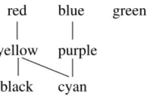
Example 1.Figure 1 expresses a simple user preference on the domain of colors dom(color) ={red, blue, green, yellow, purple, black, cyan}when searching for a car in Table 1. The colors red,blue, and greenare preferred over yellow and purple, which are better than black and cyan. Thereby, all colors in the same set should be considered as equally good and as substitutable (we refer to this as regular Substitutable Values (SV) semantics later on in this paper [23]).
(0)
(1)
(2)
L1={red, blue, green}
L2={yellow, purple}
L3={black, cyan}
ABetter-Than Graph (BTG, also known as Hasse diagram) is a visual rep-resentation of the domination of domain elements for a preference as can be seen in Figure 1. Thenodes in this BTG representequivalence classes. Each equiv-alence class contains objects which are mapped to the same level by a utility
function. Theedgesin the BTG state dominance.
The preference order in Figure 1 forms a weak order, because all values in the same equivalence class are considered as substitutable and for each equivalence class we can specify a numerical value which represents a node in the BTG. In real life a user does not have necessarily such simple preferences, but specifies his wishes in a more explicit way.
Example 2. A general strict partial order which does notform a weak order
is given in Figure 2. In fact, red, blue, and green are the best values, but
they are not considered as substitutable (trivial SV-semantics). In addition, green is not better than yellow or purple, i.e., the ’best values’ cannot lie in the same equivalence class, we cannot represent red,blue, and green with one single numerical value as in Figure 1.
cyan blue yellow red green purple black
Figure 2: Hasse diagram for a general SPO.
Based on such simple preferences on single domains, we can build complex preferences on multiple attributes of a database relation. For example, the Pareto preference renders all included preferences asequally important. In the literature this kind of data selection is also called theSkyline operator [2]. Typi-cally such techniques are used to find optimal tuples w.r.t. potentially conflicting goals.
There are many algorithms for the computation of preference queries (see [6] for an overview). Many of them rely on a nested-loop and tuple-to-tuple com-parison approach (e.g., Block-Nested-Loop, BNL [2]). The major advantage of the BNL algorithm is its simplicity and suitability for computing the maxima of general strict partial orders. However, most of the tuple-comparison algorithms have a quadratic worst-case time complexity, O(n2d) – where n is the size of thed-dimensional input data.
On the other hand there are many algorithms which exploit the lattice structure induced by a Pareto preference for efficient preference evaluation, cp. [30, 33, 12, 11, 26, 21, 14]. In a lattice, two arbitrary elements have an infimum and a supremum. Most of these algorithms o↵er excellent performance for domains with low cardinalities. The lattice based algorithms are the only ones with a linear runtime complexity, O(dV +dn), where V is the product of the cardinalities of thed low-cardinality domains. Apart from the domain
size restriction, lattice based algorithms can only deal withPareto preferences consisting of preferences that form weak orders on their domains. But this is not always suitable for real life applications as in Figure 2.
In this paper, we present a method to embed any strict partial order into a lattice. That means, we overcome the weak order restriction and thus make lattice-based algorithms capable of dealing with general strict partial orders. For this, we show 1.) how to transform general strict partial orders into lattice structures, 2.) how to construct smaller lattices in the case of special base preferences, and 3.) how to combine weak orders and general strict partial orders into lattices.
The rest of this paper is organized as follows: Section 2 contains the formal background. Section 3 presents the embedding of general database preferences into lattices, and in Section 4 we present a method to construct smaller lattices for base preferences. In Section 5 we show how to combine weak order prefer-ences and general strict partial orders. In Section 6 we discuss some implemen-tation details. Section 7 provides some related work and Section 8 contains our concluding remarks.
2
Background
Preference queries in database systems have been in focus for some time, leading to diverse approaches, e.g., [5, 22]. We review [22, 23], where preferences are modeled as strict partial orders.
2.1
Preference Modeling
Following [22] a database preferenceP is defined as P := (A, <P), where Ais
a set of attributes and<P is astrict partial order (SPO) on the domain ofA.
The termx <P yforx, y2dom(A) is interpreted as “I like y more than x”, “is
preferred to”, or “is more probable than”, and so forth. As strict partial orders aretransitive, better-than relations in this model are, too. Themaximal values ofP= (A, <P) are defined as
M(P) :={v2dom(A)|6 9w2dom(A) :v <P w} (1)
If of two di↵erent objects none is better w.r.t. a preference, we call them indif-ferent, cp. [22, 10, 15]. Theindi↵erence relationkP is defined as:
xkP y,¬(x <P y_y <P x)
2.2
Weak Order Preferences
An important subclass of strict partial orders areweak order preferences(WOP). Following [15, 16], a weak order preference is a strict partial order in which
indi↵erence is transitive. For any WOP we can define a utility function [15]
mapping each attribute value to a number to determine dominance between two values. The utility function depends on the type of preference as can be seen in the next section.
Lemma 1(Utility Function for WOPs [15]). Each weak order preferenceP = (A, <P)has a utility function to determine the dominance between values:
uP : dom(A)!R+0
x <P y()uP(x)> uP(y)
For weak order preferences indi↵erent values belong to the sameequivalence class. The equivalence class of an attribute valuexcan be identified byuP(x).
Note that if P is a weak order then kP is an equivalence relation (reflexive,
symmetric, transitive).
Definition 1 (max(P)). max(P) 2R0 is the maximum uP value for a weak
order preferenceP.
max(P) := max{uP(v)|8v2dom(A)}
2.3
Base Preferences
Preferences on single attributes likediscrete (categorical) orcontinuous (numer-ical) domains are called base preferences, cp. [24]. Usually they can be defined as WOPs having a utility function, such that
uP(v) := ( f(v) if d= 0 lf(v) d m if d >0 (2)
wheref : dom(A)!R+0 is a score function and d2R+0. In the case of d= 0 the functionf(v) models thedistance to the best value. A d-parameter d >0 represents a discretization, which is used to group ranges of scores together. The
d-parameter maps di↵erent function values to a single integer number. Choosing
d >0 e↵ects that attribute values with identicaluP(v) value becomeindi↵erent
and stay in the sameequivalence class.
The definition of the function f depends on the type of preference. The BETWEENd(A,[low,up]) preference for example expresses the wish for a value
between a lower and an upper bound. If this is infeasible, values having the smallest distance to [low,up] are preferred, where the distance is discretized by the parameter d. The scoring function is f(v) = max{low v,0, v up}. The AROUNDd(A, v) is a special case of the former, where low = up =: v.
for the minimum and maximum, where infA and supA are the infimum and
supremum of dom(A).
In a categorical domain LAYEREDm(A,{L1, . . . , Lm}) expresses that a user
has a set of preferred values given by the disjoint setsLi, which form a partition
of dom(A). Thereby the values inL1are the most preferred values. The scoring function equalsf(v) =i 1 ,x2Li. Figure 1 shows an example for such a
preference.
2.4
Complex Preferences
Complex preferences combine other preferences and determine the relative im-portance of these. Intuitively, people speak of “this preference is more important to me than that one” or “these preferences are all equally important” (Pareto) [22, 5]. Hence, we need a notion of equality w.r.t. a preference.
A simple approach for the notion of equality w.r.t. a preference is to use strict equality of the domain values. But equivalence classes can be applied here as well. For example, if for two values x, x0, uP(x) = uP(x0), i.e., the
tuples have the same utility value; they belong to the same equivalence class and hencex <P y,x0 <P y for ally.
The substitutable value semantics has been introduced in [23] to have
in-di↵erence as a transitive relation and every preference P is associated with
an SV-relation⇠=P on dom(A), where the equivalence classes contain “equally
good” objects.
Definition 2(Substitutable Values (SV)).
Let P = (A, <P). ⇠=P isP’s substitutable values relation (SV) i↵ 8x, y, z2 dom(A)
a) x⇠=P y ) xkP y
b) (x <P y ^ y⇠=P z)_(x⇠=P y ^ y <P z))x <P z
c) ⇠=P is reflexive, symmetric, and transitive
The identity relation on attribute setA is called trivial SV-relation (=P). The
regular SV-relation ⇠P is the equivalence relation induced by the equivalence
classes computed byuP.
Note that this definition of SV-semantics is needed to preserve the strict order property of complex preferences, cp. [23, 15].
The intuition behind SV-relations is that a tuple x can be substituted by
x0, if x⇠=
P x0 holds. For base preferences regular SV-semantics ⇠P does not
a↵ect<P itself, but expresses that it is admissible to substitute values for each
other. The di↵erence occurs when such preferences are combined to complex preferences, e.g., a Pareto preference, where ⇠P does a↵ect <P. Then, the
Definition 3 (Pareto Preference). Given m preferences Pi = (Ai, <Pi) and objects x = (x1, . . . , xm), y = (y1, . . . , ym)2 dom(A1⇥· · ·⇥Am). A Pareto
preferenceP :=P1⌦. . .⌦Pm is defined as: x <P y () 9i:xi<Pi yi ^
8i, j2{1, . . . , m}, j6=i: (xj<Pj yj _ xj⇠=Pj yj)
Note that although we have only WOPs as input preferences for a Pareto preferenceP,P itself forms a strict partial order, but not a WOP anymore [5]. All input values leading to the same utility value combination (uP1(v), . . . , uPm(v)) for the WOPsPi in P belong to the same equivalence class.
Example 3.Reconsider Example 1. The preferenceP1on colors (Figure 1) now should be equally important toP2:= AROUND5(price,50K)(Pareto preference query). Let x = (red,50K) and y = (blue,45K) be two tuples as in Table 1. Using trivialSV-semantics the tuple (red,50K) is not better than(blue,45K), although a price of$50K (uP1(50K) = 0) is better than $45K (uP1(45K) = 1). Due to the trivial SV-semantics ’red’ and ’blue’ are notsubstitutable. Note that the same holds for(green,48K), i.e., the result are the cars with id2{3,4,7}. Having regular SV-semantics, ’red’ and ’blue’ (and ’green’) become substi-tutable in the preference on the colors. Hence, (red,50K) is equally good as (blue,45K) concerning the color, but a price of$50K is better than $45K con-cerning the preference AROUND5. This means, (red,50K) is the only tuple in the result set which corresponds to the car with id = 3. It also dominates (green,48K).
2.5
Better-Than-Graph and Lattices
ABetter-Than-Graph(BTG) is a visualization of the partial order induced by
a preference. A graph like this is equivalent to aHasse diagram (directed and acyclic) [10]. An edge between two nodes in a BTG denotes dominance of the upper node over the lower.
Definition 4 (Better-Than Graph (BTG)). The better-than graph of a pref-erenceP = (A, <P) is the Hasse diagram of <P with the additional
character-istics:
a) A node in the BTG corresponds to a value or a set of substitutable values (equivalence class) indom(A).
b) The utility function value of a node is the length of a longest path leading from the best node to it.
The BTG for weak order preferences forms a total order where each node represents one equivalence classuP, cp. Figure 1. A Pareto preferencePhas one
node for each possibleutility value combination of thePis ofP and constitutes
a lattice [10, 30], where each node in the BTG stands for one equivalence class of the preference.
Definition 5 (Lattice [10]). A partially ordered set D with operator <P is a
lattice, if 8a, b 2 D, the set {a, b} has a least upper bound (supremum) and a greatest lower bound (infimum) inD. If a least upper bound and a greatest lower bound is defined for all subsets ofD, we have a complete lattice.
Lemma 2 (#Nodes of a BTG [33]). Let P := P1 ⌦. . .⌦Pm be a Pareto
preference on the domain dom(A) := dom(A1)⇥. . .⇥dom(Am) and Pi, i =
1, . . . , m WOPs withmax(Pi) as in Definition 1. Then
#nodes(BT GP) = m
Y
i=1
(max(Pi) + 1) (3)
More properties of BTGs (#edges, height, width, etc.) can be found in [33].
Example 4. Consider our car sample in Table 1. Let P1 be a LAYERED3 preference as in Figure 1, i.e., theuP mapping is as follows:
red, blue, green ! 0
yellow, purple ! 1
black, cyan ! 2
LetP2 be aLAYERED5preference on themakein Table 1, where each make
forms its own layer in the order GMC! 0, BMW !1, Ford !2, Mercedes
!3, Audi!4.
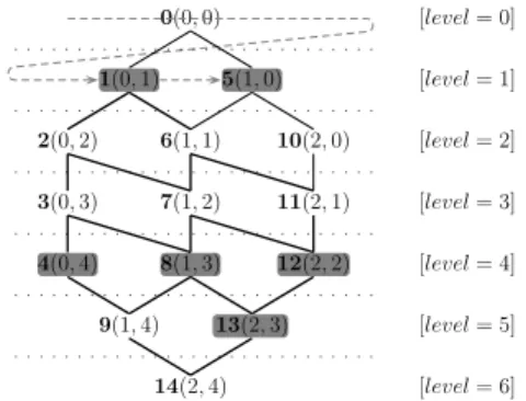
Figure 3 shows the BTG for the Pareto preferenceP1⌦P2with the maximum valuesmax(P1) = 2 andmax(P2) = 4. The node(0,0) presents the best node, i.e., the supremum, whereas(2,4) is the worst node (infimum). The bold num-bers next to each node are unique identifiers (ID) for each node in the lattice, cp. [33].
A datasetDdoes not necessarily contain tuples for each lattice node. In Fig-ure 3, the gray nodes are occupied (non-empty) with elements from the dataset
in Table 1 whereas the white nodes have no element (empty). Each node
con-tains the objects mapped byuP to the same feature vector of the preference query.
For example, the tuples (red,BMW) and(green,BMW)both correspond to the
node(0,1). All values in the same node / equivalence class are indi↵erent and considered substitutable. The number of nodes is(2 + 1)·(4 + 1) = 15.
2.6
Lattice Skyline Revisited
Lattice based algorithms like LS-B [30] and Hexagon [33] exploit the observa-tions from the last section to find the maximal values of a dataset w.r.t. some preferences. The elements of the dataset D that compose the maximal values is formed by those nodes in the BTG that haveno path leading to them from another non-empty node. All other nodes have direct or transitive edges from the maximal nodes, and therefore aredominated.
For the implementation of such algorithms the lattice is usually represented by an array, where each position stands for one node in the lattice [30] (ac-cording to the ID for each node as in Example 4). The array stores the
2(0,2) 3(0,3) 4(0,4) 1(0,1) 9(1,4) 0(0,0) 6(1,1) 7(1,2) 8(1,3) 14(2,4) 5(1,0) 13(2,3) 10(2,0) 11(2,1) 12(2,2) [level= 6] [level= 5] [level= 4] [level= 3] [level= 2] [level= 1] [level= 0]
Figure 3: BTG for a Pareto preference.
empty, non-empty, and dominated state of a node. For each element t 2 D
the algorithms compute the unique position in the array and mark this posi-tion asnon-empty. Next, the nodes are visited in a breadth-first order (BFT, dashed line in Figure 3). Non-empty nodes cause a depth-first traversal (DFT, thick black edges in Figure 3) where the dominance flags are set. Finally those nodes represent the maximal values which are bothempty and non-dominated. In Example 4, only the nodes (0,1)'{(red,BMW),(green,BMW)}
and (1,0)'{(yellow,GMC)} are not dominated. All other nodes have direct or transitive edges from these two nodes, and therefore are dominated. Note that in general strict partial orders do not form lattices (e.g., Figure 2) and therefore the above approach cannot be applied.
The original lattice based algorithms have linear runtime complexity w.r.t. the number of input objects and the size of the BTG. More precisely, the complex-ity is O(dV +dn), where d is the dimensionality, n is the number of input tuples, and V is the product of the cardinalities of the d domains from which the attributes are drawn.
3
General Strict Partial Orders
In Section 2 we have seen that the BTG of a Pareto preference is a lattice. Now, we will use such lattices as an abstraction from the underlying preference to integrategeneral strict partial orders. This will enable us to handle arbitrary preferences in the same way as Pareto preferences.
3.1
Embedding General SPOs into Lattices
To define general strict partial orders the preference constructor EXPLICIT(A, E) was introduced in [22]. It constructs a preference from a given set of edgesE. Unmentioned values are considered worse than any value in some element of
E. The transitive hull ofE is the Better-Than-Graph of the strict partial or-der expressed by EXPLICIT. In contrast to other base preferences it doesnot construct a weak order.
Example 5. A typical simple general strict partial order expressed asEXPLICIT is
I like redmore thanblack. And I like blue.
Figure 4 shows the Hasse diagram of this preference, which does not construct a weak order.
blue black
red
Figure 4: Hasse diagram for a general SPO.
Unfortunately there is no efficient algorithm to evaluate arbitrary database preferences as above but BNL, because BNL compares each tuple to all other tuples in the dataset (worst-case complexity O(dn2), cp. [2]). To be able to apply efficient algorithms like [30, 33, 12, 11, 14] on EXPLICIT, we have to embed the strict partial order defined by it into a distributive lattice.
For this embedding, we start with a Hasse diagram representing a general strict partial order. Since lattices need a least upper bound and a greatest lower bound (cp. Definition 5) we just add virtual nodes to the existing Hasse diagram. Then, we will assign a so-calledsignatureto each node. This signature is a combination of integers that isunique for each node and hence can be used to identify it.
For nodes in the same level (which are indi↵erent) we construct Pareto in-comparable signatures. A node n which is directly dominated by a node m
needs a “worse” signature than the dominator. For this we just increase one position in the signature of m and assign it to n. Which position we use is determined by a depth-first traversal. When the construction of the distributed lattice structure is complete, the signature of a node is identical to the
inte-ger combination of the BTG node it is mapped to. Algorithm 1 describes our
approach in detail.
Algorithm 1. (Embedding SPOs into Lattices).
The mapping is done in the following steps:
1) Identify non-dominated nodes and generate an unlabeled virtual top node4
for them. Add edges from4to the non-dominated nodes. Also add a virtual bottom node5that is dominated by all the nodes not dominating other values in the graph.
2) Do a depth-first search beginning at the top node. The algorithm used for the depth-first search is irrelevant, but the following issues have to be kept in mind:
a) Keep a counter. Each time the search finds a dead end, increase the counter by one.
b) Annotate each edge during the search with the counter value. c) Do not follow annotated edges.
3) Do a breadth-first search on the graph, starting at the top node again. There are two possibilities in each noden:
a) n is directly dominated by exactly one node and reached by an edge with an annotated value of v. The signature value ofn is the signature value of its dominating node increased by one at position v.
b) n is directly dominated by a number of nodesd1,d2, . . . ,dx. The
signa-ture of n at each position i is given by the maximum value of the di at
the same position.
If two nodes n and m (or more) are dominated directly by exactly the
same set of nodes d1, . . . , dx, this yields the same signature. In this case,
increase the value of n (resp. m) at the position of the edge on which it was reached first by the depth-first search.
4) Check the maximum values in use at each position of the node signature and remove those positions with a maximum value of zero.
Please note that in step 3b also signature values at other positions could be increased. This can lead to smaller BTGs. It is only necessary that n’s and
m’s signatures are increased at di↵erent positions, preserving their indi↵erence. Step 4 is unnecessary for the correctness of the algorithm. It is simply removing elements not containing any information for any node to reduce the signature length. For an EXPLICIT preference, all domain values not mentioned in its constructor are mapped to the virtual bottom node.
We now prove that Algorithm 1 preserves the original strict partial order.
Proof. We have to show that 1.) the signatures can be used to determine a
supremum and an infimum for each pair of nodes, which is the basic character-istic of a lattice, cp. Definition 5. Apart from that, 2.) the relation between any two nodes of the SPO has to be preserved.
1.) Let’s assume for a SPO our algorithm yields node signatures withn posi-tions. Using the signatures, the supremum for any two nodesaand bwith signatures (a1, . . . , an) and (b1, . . . , bn) is defined as
sup(a, b) := (min(a1, b1), . . . ,min(an, bn)),
their infimum as
Both infimum and supremum of two nodes might not be elements of the original SPO (like4 and 5), cp. [10]. The top node 4 by definition has the signature (t1, . . . , tn) = (0, . . . ,0). The supremum of any nodexand4
is4, while their infimum isx. In this sense Algorithm 1 constructs a lattice from the node signatures.
2.) Given two nodesa and b in the SPO withb <P a. Then there is a path
fromatob.
• For any nodeg= (g1, . . . , gn) on this path that is dominated by exactly
one node, the signature is increased at the position given by the edge’s annotation. Assume this position is i. So for all such nodesg on that path it holds that gi> ai. This holds forbas well.
A node h on the path dominated by two nodes f0 and f00 will have signature values defined by the maximum values of the dominating nodes (a generalization to more than two nodes is obvious). As f0 k
P f00, it holds that 9i, j:f0 i > fi00 ^ fj0 < fj00,and 8k:hk fk0 ^ hk fk00 ^ (9i, j:hi> fi00 ^ hj> fj0).
In summary, nodes which are dominated by one or more nodes in the original SPO are modeled as dominated in the lattice structure, too.
• We have to consider indi↵erent nodes in the original SPO. For this consider two nodes skP t. We can find a supremum as
x:= sup(s, t) := (min(s1, t1), . . . ,min(sn, tn)).
We assume a path fromxtosstarting with an edge annotated withi, reaching the node x0 with
x0 :=
(min(s1, t1), ...,min(si, ti) + 1, ...,min(sn, tn))
A path from xtotstarts with an edge annotated with j, leading to a node
x00:=
(min(s1, t1), ...,min(sj, tj) + 1, ...,min(sn, tn))
Note that i6=j, as otherwisex0 and x00 would be the equal node and the supremum of sand t. So x0 k
P x00 in the lattice, sincex0 and x00
cannot dominate a node that dominates bothsandtas this would be their supremum. Hencesandt must be indi↵erent.
Based on our algorithm we are now able to embed any strict partial order into a lattice. After constructing the lattice and mapping the nodes to an array as described in Section 2.6, we apply a lattice based algorithm like LS-B or Hexagon. The remaining nodes contain the maximal values. Note that our approach still has a linear runtime complexity. The construction of the lattice in Algorithm 1 only relies on a DFT and a BFT, both are linear in the number of nodes and edges.
The exponential lattice size is not a major limitation, because in most cases preferences are specified only over a few items, all others can be considered as worse then the mentioned objects and hence can reside in the virtual bottom node of the lattice. That means, it is not necessary to construct the lattice on the complete domain, but only on the objects specified by the user. Therefore we create small lattices which can be handled efficiently.
3.2
Examples
We now present some examples on how to embed general strict partial orders into BTGs.
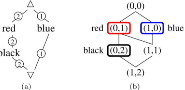
Example 6. Reconsider the preference given in Figure 4. Following Algorithm 1, we add a virtual top and bottom node. Then, the depth-first traversal anno-tates all edges as shown in Figure 5a. The highest annotation is 2 and hence the virtual top node corresponds to4 !(0,0). Then the mapping into a lattice is “red”!(0,1), “blue”!(1,0), and “black” !(0,2). In this case the signa-ture for the virtual bottom node isO!(1,2) which characterizes the complete structure of the lattice. Figure 5b shows the lattice with the order embedded into it. The nodes with frames represent the original Hasse diagram’s nodes.
2 2 1 1 2
black
red
blue
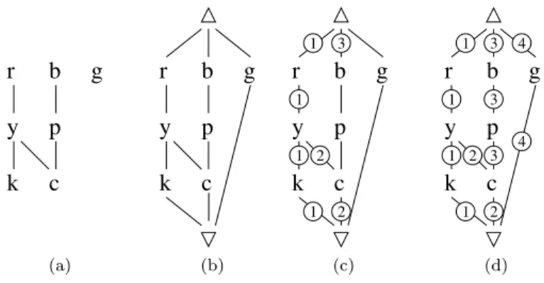
(a) (1,0) (0,1) (0,0) (0,2) (1,1) (1,2) black red blue (b)Example 7. Another Hasse diagram for a general partial order is known from the introductory Example 2 and presented again in Figure 6a, where we use the abbreviations red (r), blue (b), green (g), black (k), etc.
c
r
y
k
b
p
g
(a)c
g
r
b
y
p
k
(b)c
g
r
b
y
p
k
1 1 1 2 3 1 2 (c)c
k
p
y
b
r
g
1 4 4 3 3 3 2 1 1 1 2 (d)Figure 6: Embedding a SPO into a BTG (1).
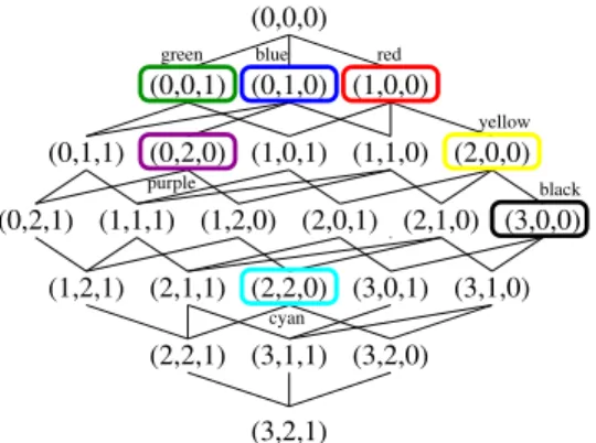
Following Algorithm 1, we add top and bottom nodes in Figure 6b. Then, the depth-first marking of the edges begins. Figure 6c shows the moment when the counter value is “3” and the first edge has been marked with it. In Figure 6d, all edges are marked. The depth-first orders leads to annotations on the edges which make each path from the top node to any other node in the Hasse diagram unique.
Then, we determine the node signatures, starting at4. As the highest num-ber assigned to an edge is 4, the node signatures consists of four integer values. The top node has a signature of(0,0,0,0). Forr, we get the signature(1,0,0,0), as it is dominated by the top node by an edge marked with1and so the signature value of4 is increased by one at position 1. Table 2 shows signatures for all nodes after step 3 of the algorithm.
Table 2: Signatures for all nodes after step 3.
node r y k
signature (1,0,0,0) (2,0,0,0) (3,0,0,0)
b p c g
(0,0,1,0) (0,0,2,0) (2,0,2,0) (0,0,0,1)
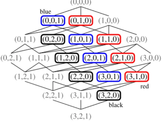
We see that the maximum value at position 2 is 0. Hence it is removed. So we keep the maximum signature values 3, 2, and 1. The resulting BTG can be seen in Figure 7 showing all signature values and the framed nodes connected to a value of the original order. Note that themax(P)values are 3, 2, and 1, hence the BTG has4·3·2 = 24 nodes.
(3,0,1) (1,1,0) (1,0,1) (3,1,0) (2,2,1) (3,1,1) (3,2,0) (0,0,1) (0,1,0) (1,0,0) (0,0,0) (0,2,0) (2,0,0) (3,0,0) (2,2,0) (0,1,1) (3,2,1) (1,2,0) (2,1,1) (1,2,1) (2,1,0) (2,0,1) (1,1,1) (0,2,1) red black cyan purple green blue yellow
Figure 7: Lattice structure for the preference expressed in Figure 6a.
Our algorithm has no problem in integrating any kind of strict partial order. Isolated nodes in a Hasse diagram belong to the set of top nodes that is linked to the virtual single top node created in step one of the algorithm. Please note that our algorithm for embedding a strict partial order into a distributive lattice like a BTG is not necessarily producing minimal BTGs.
Example 8. We will have another look at the strict partial order in Figure 6a. Some depth-first search algorithm yields the edge annotation of Figure 8. Then, the maximum integer values for the embedding are 2, 1, 2, 1. With those maximum values, the BTG that is constructed has 36 nodes; it is 50% bigger than the one shown in Example 7.
c
k
p
y
b
r
g
1 3 3 3 4 4 2 2 1 1 13.3
Remarks
Another mapping of partial orders to distributive lattices has been presented in [36]. Using only two integer numbers to represent each value in a partial order, a BTG constructed according to the maximum signature levels tends to be smaller than when using Algorithm 1. But not all partial orders can be expressed when such a mapping is used, as we will see in Lemma 3.
Lemma 3. We have some values a, b, . . . , f and a partial order on them defined byd < a,d < b,e < a,e < c,f < b, and f < c. The Hasse diagram for this order is given in Figure 9. Then a mapping of each node to a BTG node defined by two integer values is not able to preserve the original partial order.(0,0,0)
f e d c b a (1,1,1)
Figure 9: SPO needing more than two integer values.
Proof. Leta= (a1, a2),b= (b1, b2), andc= (c1, c2) the indi↵erent two integer representations of the corresponding nodes. We will assumea1 < b1 < c1 and a2> b2> c2. From the strict partial order we know:
e < a^e < c)a1e1^a2e2^c1e1^c2e2
Hence, the combination of smallest possible values foreis (e1, e2) = (c1, a2). So ealways is dominated byb, too, which is a contradiction to the original partial ordered set.
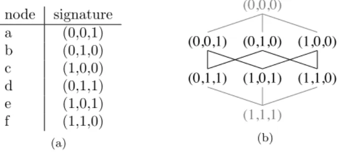
Using the Hasse diagram structure of Figure 9 as a pattern, similar proofs for more than two values in a signature can be found. The number of integers needed to construct a BTG to embed a partial order depends on the partial order and does not have an upper border. In Example 9, a possible embedding of the given partial order into a BTG using three integer values can be seen.
Example 9. Consider the partial order in Figure 9. A possible embedding to a distributed lattice is shown in Figure 10. The maximum values are(1,1,1).
4
WOPs with Trivial SV-Semantics
Our approach of embedding general SPOs does not necessarily construct mini-mal lattices. We assume that finding a minimini-mal lattice is an NP-hard problem. Therefore, we leave this for further investigations and future work. Never-theless, in this section we show a method which in general constructs smaller lattices than Algorithm 1. However, this only applies for base preferences like LAYEREDmand BETWEENd and their sub-constructors.
node signature a (0,0,1) b (0,1,0) c (1,0,0) d (0,1,1) e (1,0,1) f (1,1,0) (a) (1,1,0) (0,0,0) (1,0,0) (0,1,0) (0,0,1) (1,1,1) (0,1,1) (1,0,1) (b)
Figure 10: Mappings (a) and lattice structure (b) for the SPO in Figure 9.
We have seen that graphs of WOPs (with regular SV-semantics (⇠=P)) build
a total order and therefore always construct a minimal lattice (cp. Section 2.5). A Pareto preference consisting of WOPs also constitutes a complete lattice, which is minimal w.r.t. the base preferences. Therefore, we now consider base preferences with trivial SV-semantics (=P). Keep in mind that for regular
SV-semantics all objects in an equivalence class are substitutable, but in the case of trivial SV-semantics they are not. That means each object in a dataset forms its own (single valued) class.
4.1
Categorical Base Preferences with Trivial SV-Semantics
Modeling incomparability of values in categorical base preferences is straightfor-ward. Using trivial SV-semantics in LAYEREDm(A,{L1, . . . , Lm}), all values
in one of theLi are incomparable.
Theorem 1. Let P := LAYEREDm(A,{L1, . . . , Lm}) andP0 derived from P
by replacing regular with trivial SV-semantics. Each value indom(A)is mapped to a pair of integer values.
The elements of the Li are labeled with indexes: Li:={li,1, li,2, . . . , li,|Li|}. Every element ofLi has to get a unique index value. Then, the integer
combi-nation for eachli,j can be found as follows: li,j!(ll, lr)
where
ll := Six=11Lx i+j
lr := Six=1Lx + 1 (i+j) +
Proof. Consider three categorical valuesli,j, li,k, li+1,q 2dom(A) withj < k. A
valuelx,y is mapped to (lx,y[0], lx,y[1]). We have to prove that P0 constructs
the same order asP on elements of di↵erent layers and renders elements of the same layer indi↵erent. For readability, we will abbreviate Six=11Lx withsand
|{x|xi^|Lx|= 1^|Lx 1|= 1}|witht(i). • li,j kP0 li,k:
– li,j[0] li,k[0] = (s i+j) (s i+k) =j k)li,j[0]< li,k[0]
– li,j[1] li,k[1] = (s+|Li|+1 (i+j)+t(i)) (s+|Li|+1 (i+k)+t(i)) = j+k)li,j[0]> li,k[0]
With li,j[0]< li,k[0]^li,j[0]> li,k[0] it follows thatli,jkP0 li,k. • li+1,q<P0 li,j:
– li,j[0]li+1,q[0],j|Li| 1 +q
This always holds asj|Li|^( 1 +q) 0
)j =|Li| 1 q,j =|Li|^q= 1 andj <|Li| 1 q,j < |Li|_q >1 • li,j[1]li+1,q[1], j+t(i)|Li+1| 1 q+t(i+ 1) – case 1: |Li|= 1^|Li+1|= 1,t(i+ 1) =t(i) + 1)j = 1^q= 1 ) j+t(i)|Li+1| 1 q+t(i) + 1 – case 2: |Li|>1_|Li+1|>1,t(i+ 1) =t(i) ) j+t(i)|Li+1| 1 q+t(i)
Forj= 1^q=|Li+1|, both sides are equal. As (j 1)^(q |Li+1| 0), the inequation holds in all other cases, too.
To sum up the preceding points, we showed that
li+1,q <P0 li,j always holds: • j= 1^q=|Li+1| =)li,j[0]< li+1,q[0]^li,j[1] =li+1,q[1] • 1< j <|Li|^1< q <|Li+1| =)li,j[0]< li+1,q[0]^li,j[1]< li+1,q[1] • j=|Li|^q= 1 =)li,j[0] =li+1,q[0]^li,j[1]< li+1,q[1]
As we can see, all elements of the same layer are indi↵erent and better than all elements of (w.r.t. their indexes) higher layers.
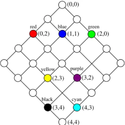
Example 10. Consider the color preference in Figure 1. We derive a preference
P0 with the same sets but trivial instead of regular SV-semantics. This means for example that ’red’, ’blue’, and ’green’ arenotsubstitutable. Table 3 shows the integer combinations (ll, lr) for each color. For example, for ’red’ we compute ll= 0 1 + 1 = 0andlr= 3 + 1 (1 + 1) + 0 = 2, i.e., ’red’!(0,2).
Table 3: Mappings for Example 10.
color Li uP li,j (ll, lr) red L1 0 l1,1 (0,2) blue L1 0 l1,2 (1,1) green L1 0 l1,3 (2,0) yellow L2 1 l2,1 (2,3) purple L2 1 l2,2 (3,2) black L3 2 l3,1 (3,4) cyan L3 2 l3,2 (4,3)
Figure 11 shows the lattice forP0. Nodes with invalid level combinations are white, nodes with other colors filled and labeled with the color and its assigned integer combination. Following Eq. 3, the size of the BTG is5·5 = 25. Note that the number of occupied nodes is the size of the categorical domain,|dom(A)|= 7.
(4,3) (4,4) (0,2) (1,1) (2,0) (2,3) (3,2) (3,4) (0,0) green black cyan yellow purple blue red
Figure 11: BTG for LAYEREDmwith trivial SV-semantics.
4.2
Numerical Base Preferences with Trivial SV-Semantics
In the case of numerical preferences it is sufficient to analyse the problem only for BETWEENd, because all other numerical base preferences are special cases
of the former. However, embedding BETWEENd into a lattice is not a trivial
task, because if two values exist in the same equivalence class, they are not sub-stitutable when using trivial SV-semantics and must be modeled incomparable in the lattice structure.
Example 11. LetP := AROUND5(price,50K)be a preference withdom(price) ={45K,48K,50K}. The value 50K is the maximal value, whereas 45K,48K
lie in a distance of d from the best value. Since45K,48K 2[45K,50K[, they
share the same uP value 1, but are not substitutable and must be modeled as
incomparable in the lattice which they should be embedded in.
Since the domain of an attribute could be infinite, this makes the embedding of numerical base preferences with trivial SV-semantics difficult. However, in database relations we generally assume aclosed-world, hence we have a finite number of objects in an equivalence class. In this case, BETWEENd could be
modeled in the same way as LAYEREDm. That means, construct a
prefer-ence LAYEREDmbased on the numerical values preferred by BETWEENdand
computeli,j as in Theorem 1.
Under some assumptions we can produce smaller lattices, e.g., when we have single occupied equivalence classes, or if a user specifies an “interval as the preferred value”. In these cases we avoid the problem of several indi↵erent objects in the same equivalence class; objects having the sameuP function value
are either identical or lie “left and right” of the maximal value.
Theorem 2. GivenP := BETWEENd(A,[low, up])and letP0 be derived from P by replacing regular by trivial SV-semantics. Assume each equivalence class
contains at most one element. We mapx2dom(A)to the integer combination
(l1, l2) inP0 as follows:
x!(l1, l2) = ⇢
(uP(x) , uP(x) 1) if x > up
(uP(x) 1 , uP(x) ) if x < low
Forx2[low, up]we setx!(0,0). Then,P0models the same order w.r.t.dom(A) asP, but distinguishes between values lower and values higher than the interval borders.
This can be interpreted as two WOPs being connected and used to model a strict partial order. A “virtual” Pareto preference is constructed by the numer-ical base preference.
Proof. Consider a valuevmapped to (v1, v2), and a valuewmapped to (w1, w2). The following cases may occur:
• uP(v) =uP(w) + 1: – v < low^w < low)(w1=v1+ 1)^(w2=v2+ 1) – v < low^up < w)(w1=v1+ 2)^(w2=v2) • uP(v) =uP(w): – v < low^w < low)(v1, v2) = (w1, w2) )v⇠P0 w
– v < low^up < w
) ((wv1, v2) = (uP(v), uP(v) + 1) 1, w2) = (uP(v) + 1, uP(v))
)vkP0 w
All other possible cases can be derived from those above. So the integer combi-nation assigned to domain values fulfills the specification of the preference.
Lemma 4 (#Nodes). The number of nodes in the BTGP0 defined by a
pref-erenceP := BETWEENd by replacing regular by trivial SV-semantics is given
by:
#nodes(BT GP) = (max(P) + 1)2 (4)
Proof. Looking at the computation of integer combinations for values to be
rated, the BTG that is constructed is identical to one for a Pareto preference containing two WOPs with maximum values of max(P) + 1, cp. Eq. 3.
Lemma 5 (#Used Nodes). Consider a preference P0 which is defined as a BETWEENd preference P with trivial instead of regular SV-semantics. The
number of used nodes (i.e. the number of nodes that can be matched by values
evaluated byP0) in the BTGP0 is given by
#used nodes(BT GP0) = 2·max(P) + 1 (5)
Proof. The node (0,0) is used for perfect matches. Other nodes used have
combinations of (x, x+ 1) or (x+ 1, x). The minimum value for x is 1, the maximum is max(P), leading to 2·max(P) + 1 values in use.
Note that Lemma 4 and 5 only hold when considering equivalence classes which contain at most one object.
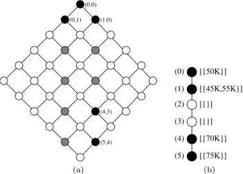
Example 12. We search for a car which should cost around$50K, i.e., P := AROUND5(price,50K)in the domaindom(price)={45K,50K,55K,70K,75K}. Thenmax(P) = 5.
No two domain values lie in the same equivalence class, we derive P0 with trivial SV-semantics and create pair mappings: A perfect value of 50K is mapped to(0,0), 45K and 55K (withuP(45K) =uP(55K) = 1) are mapped to
incom-parable value combinations(0,1) and (1,0), respectively. All combinations can be found in Table 4.
Table 4: Value combinations forP0.
price 45K 50K 55K 70K 75K
uP 1 0 1 4 5
Figure 12a shows the BTGP0 of P0 with trivial SV-semantics. The black
nodes have tuples belonging to them, the gray nodes represent valid integers for
l1 and l2, while the white nodes are unused dummy nodes given by the graph structure. The number of nodes is(5 + 1)2= 36from which2·5 + 1 = 11might be used.
In Figure 12b we present BTGP forP with regular SV-semantics for
com-parison only. Values with the sameuP value are substitutable and reside in the
same equivalence class. The BTG forms a chain.
(0,0) (5,4) (4,3) (1,0) (0,1) (a) [{75K}] [{70K}] (1) (0) (2) (3) (4) (5) [{}] [{}] [{50K}] [{45K,55K}] (b)
Figure 12: BTG for AROUNDd with (a) trivial SV-semantics and (b) regular
SV-semantics.
5
Combining WOPs and SPOs
As we have seen, a single integer value is not enough to express the semantics of strict partial orders in general. We have overcome this limitation by using two or more integer values. Now we have to integrate these preferences in the standard Pareto preference introduced in Definition 3.
Theorem 3. Consider a strict partial order S embedded into a BTG GS, a
Pareto preferenceP and the corresponding BTGGP. The order constructed by
the combination ofP andS is visualized by the product ofGS andGP.
Proof. BothGS andGP are lattices. Following [10], the product of them yields
a lattice with a combined order of both input lattices.
The BTG for such a combination surely holds unused nodes (as the BTG for the strict partial order does already). Nevertheless the embedding can be very useful as it enables us to evaluate base preferences that are strict partial orders just like Pareto preferences and Pareto preferences consisting of strict partial
orders just as if they only used standard WOPs as input preferences. Example 13 defines a BTG that is the result of the combination of a WOP and a general strict partial order.
Example 13. Remember the strict partial order on colors of Example 6. A possible lattice this order can be embedded in is shown in Figure 13a, where the nodes representing nodes of the original order are framed and labeled accordingly. The construction steps are shown in Figure 13b.
(1,0) (2,1) (2,0) (1,1) (0,1) (0,0) blue red black (a) 1 1 1 2 2
black
red
blue
(b)Figure 13: Lattice for the color preference.
Now we combine this order with a WOP with a maximum valuemax(P) = 3,
e.g., AROUND10(price,50K) as in Example 12, but with d = 10 and regular SV-semantics. The BTG forAROUND forms a chain withuP 2{0,1,2,3}.
The lattice for the combined (Pareto) order can be seen in Figure 14. As the resulting BTG is the product of the BTGs of the two underlying preferences, each of the original nodes in Figure 13a is multiplied. For example, the mul-tiplication of (0,1) by {0,1,2,3} results in (0,0,1), (1,0,1), (2,0,1), (3,0,1). Nodes representing no reachable integer combination (due to the strict partial order) are printed in gray.
(1,0,0) (0,2,1) (0,1,1) (3,2,0) (1,2,0) (2,0,1) (2,1,0) (1,1,0) (1,0,1) (3,0,1) (3,1,0) (0,0,1) (0,1,0) (0,2,0) (2,2,0) (3,2,1) (3,1,1) (2,2,1) (1,2,1) (2,1,1) (3,0,0) (2,0,0) (0,0,0) (1,1,1) blue black red
6
Optimizations
As we have seen our algorithms do not produce minimal lattices. However, we propose some improvements for the lattice-based algorithms, which can be applied if the lattice is “nondense”.
6.1
Reduction on Existing Values
In many cases, only a small number of domain values actually appear in a relation. For weak orders on numerical domains, this can have the e↵ect that only some of the possibleuP values are met.
Example 14. Consider P = AROUND1(A,4) with trivial SV-semantics and let dom(A) = {5,10,15,20} be a numerical domain. Using Theorem 2 would lead tomax(P) = 16levels, i.e., a BTG of size289, even though there are only four di↵erent values in the domain withuP(5) = 1, uP(10) = 6,uP(15) = 11,
anduP(20) = 16. A mapping of these values to 0,1,2, and 3 would reduce the
size of the lattice to16.
One way to gain information of unused domain values could be the use of a histogram or a simple B-tree index. With this we can find existinguP values
for the corresponding WOPs. Then we can efficiently reduce BTG sizes by “removing” unused nodes, leading to less memory needed and less e↵ort for preference evaluation using lattice-based algorithms. The mapping of domain values to the few requireduPvalues could be done using minimal perfect hashing
functions, leading to constant access times and minimum memory requirements [8, 9, 18]. Note, that this method is also valid for BETWEENd without the
assumption ofsingle occupied equivalence classes, cp. Section 4.2.
6.2
Data Structure
In the implementation of the original lattice Skyline algorithmsHexagon [33] andLS-B[30], the lattice is represented by anarray, where each position stands for one node in the lattice, cp. Section 2.6. Following [33], the array based implementation needs at least a memory of⌃14Qmi=1(max(Pi) + 1)⌥bytes, where
thePi’s are the participating preferences.
Since our approach produces “nondense lattices”, i.e., there are many empty nodes (cp. for example Figure 7 and 12a), using an array as data structure makes no sense. Therefore we propose the approach of level-based storage. An array models thelevels (computed byuP, Eq. 2) of the BTG. Then thenodes
are stored in a HashMap or SkipList [34], cp. Figure 15.
Adding an element to the BTG means computing the level it belongs to and marking the node at the right position as non-empty or dominated. The advantage of the level-based storage using SkipLists in contrast to HashMaps lies in the reduced memory requirements, because we do not have to initialize the whole data structure in main memory. A node is initialized on-the-fly if it is marked asnon-empty or dominated. Additionally, if each node in a level is
[uP= 6] [uP= 5] [uP= 4] [uP= 3] [uP= 2] [uP= 1] [uP= 0] NIL NIL c k p y g b r NIL
Figure 15: Level-based storage of the BTG in Figure 7 using SkipLists.
dominated, we can remove all nodes from the corresponding SkipList, mark the level-entry in the array asdominated and free memory.
Using a level-based representation of the BTG with a HashMap for each level, we have a constant access for each level andO(1) for the look-up in the HashMap, since we can use a perfect hash function due the known width of the BTG in each level, cp. [19]. In summary this leads to a runtime complexity of O(dV +dn), too. For the SkipList based BTG implementation we have
O(dV +dnlogw), since operations on SkipLists areO(logw) [34], where w is the number of elements in the SkipList, i.e., the width of the BTG in the worst case.
7
Related Work
Skyline queries and the more general concept of preferences are well-known in the database community since more than a decade. There are many algorithms to compute theSkyline set, cp. [6] for an overview. The most prominent algo-rithms are based on a block-nested-loop style tuple-to-tuple comparison (e.g., BNL [2], or [25, 7, 20]). Based on this several algorithms have been published for parallel Skyline computation [37, 29, 4] or utilizing an index structure [31, 28]. The BNL algorithm is the only one who can evaluate general strict partial orders due to its tuple-to-tuple comparison approach [5]. Most of the other algorithms are restricted to Pareto preferences, because they rely on the uP value of an
object.
Other algorithms exploit the lattice structure induced by a Skyline query, cp. e.g. [33, 30]. Instead of direct comparisons of tuples, a lattice structure represents the better-than relationships. There is also work on parallel prefer-ence computation exploiting the lattice [12] and the authors of [14] present how to handle high-cardinality domains. Also the work of [39, 27, 13] exploit the lattice to compute top-k (subspace) Skylines.
The most similar work to ours is [1], [3], and [36]. In [1, 17, 32] the authors create a spanning tree on a direct acyclic graph where each node is associated with an interval. The authors of [3] map all data points in a new space, where each partially ordered value is substituted by associated coordinates. Their aim
was Skyline processing on partially ordered domains. Also [36] handle partially ordered domains using topological sorting. In [35] the author presents a method for the decomposition of strict partial orders into fundamental preference con-structs. For this the author studies which preference operators and operands are necessary to express any strict partial order. Non of these papers produce lattice structures, but ’arbitrary’ graphs.
8
Conclusion and Future Work
In this paper we presented a method to embed all kinds of strict partial orders into lattices. As a consequence, existing lattice based algorithms can be applied to general strict partial orders and prior restrictions on weak order preferences and their combinations in Pareto preferences do not apply anymore.
As we have mentioned, the lattices we construct with our algorithm are not minimal. Nevertheless a reduction of the lattice size is wise as the size of a lattice for a Pareto preference grows exponentially with the lattice sizes of the underlying preferences. Hence our next step will be to address this and improve our algorithm so that it produces minimal lattices embedding strict partial orders. However, this could be a challenging task.
References
[1] R. Agrawal, A. Borgida, and H. Jagadish. Efficient Management of Tran-sitive Relationships in Large Data and Knowledge Bases. InProceedings of SIGMOD ’89, pages 253–262, New York, NY, USA, 1989. ACM.
[2] S. B¨orzs¨onyi, D. Kossmann, and K. Stocker. The Skyline Operator. In Proceedings of ICDE ’01, pages 421–430, Washington, DC, USA, 2001. IEEE.
[3] C. Y. Chan, P.-K. Eng, and K.-L. Tan. Stratified Computation of Skylines with Partially-ordered Domains. In SIGMOD ’05, pages 203–214, New York, NY, USA, 2005. ACM.
[4] S. Chester, D. Sidlauskas, I. Assent, and K. S. Bøgh. Scalable Paralleliza-tion of Skyline ComputaParalleliza-tion for Multi-Core Processors. In Proceedings of ICDE ’15, pages 1083–1094, 2015.
[5] J. Chomicki. Preference Formulas in Relational Queries. In TODS ’03: ACM Transactions on Database Systems, volume 28, pages 427–466, New York, NY, USA, 2003. ACM Press.
[6] J. Chomicki, P. Ciaccia, and N. Meneghetti. Skyline Queries, Front and Back. SIGMOD, 42(3):6–18, 2013.
[7] J. Chomicki, P. Godfrey, J. Gryz, and D. Liang. Skyline with Presorting.
[8] R. J. Cichelli. Minimal Perfect Hash Functions Made Simple. Commun. ACM, 23(1):17–19, 1980.
[9] Z. J. Czech, G. Havas, and B. S. Majewski. An Optimal Algorithm for Gen-erating Minimal Perfect Hash Functions. Information Processing Letters, 43(5):257–264, 1992.
[10] B. A. Davey and H. A. Priestley.Introduction to Lattices and Order. Cam-bridge University Press, CamCam-bridge, UK, 2nd edition, 2002.
[11] M. Endres and W. Kießling. Semi-Skyline Optimization of Constrained Skyline Queries . InProceedings of ADC ’11. ACS, 2011.
[12] M. Endres and W. Kießling. High Parallel Skyline Computation over Low-Cardinality Domains. InProceedings of ADBIS ’14, pages 97–111. Springer, 2014.
[13] M. Endres and T. Preisinger. Behind the Skyline. InProceedings of DBKDA ’15. IARIA, 2015.
[14] M. Endres, P. Roocks, and W. Kießling. Scalagon: An Efficient Skyline Algorithm for all Seasons. InProceedings of DASFAA ’15, 2015.
[15] P. Fishburn. Preference Structures and their Numerical Representation. Theor. Comput. Sci., 217(2):359–383, 1999.
[16] P. C. Fishburn. Intransitive Indi↵erence in Preference Theory: A Survey. Operations Research, 18(2):207–228, 1970.
[17] P. C. Fishburn. Interval graphs and interval orders.Discrete Mathematics, 55(2):135 – 149, 1985.
[18] E. A. Fox, L. S. Heath, Q. F. Chen, and A. M. Daoud. Practical Minimal Perfect Hash Functions for Large Databases. Commun. ACM, 35(1):105– 121, 1992.
[19] R. Gl¨uck, D. K¨oppl, and G. Wirsching. Computational Aspects of Ordered Integer Partition with Upper Bounds. In SEA ’13: 12th International Symposium on Experimental Algorithms, pages 79–90, 2013.
[20] P. Godfrey, R. Shipley, and J. Gryz. Algorithms and Analyses for Maximal Vector Computation. The VLDB Journal, 16(1):5–28, 2007.
[21] H. Han, H. Jung, H. Eom, and H. Y. Yeom. An Efficient Skyline Framework for Matchmaking Applications. J. Netw. Comput. Appl., 34(1):102–115, Jan. 2011.
[22] W. Kießling. Foundations of Preferences in Database Systems. In Proceed-ings of VLDB ’02, pages 311–322, Hong Kong, China, 2002. VLDB.
[23] W. Kießling. Preference Queries with SV-Semantics. In Proceedings of COMAD ’05, pages 15–26, Goa, India, 2005. Computer Society of India. [24] W. Kießling, M. Endres, and F. Wenzel. The Preference SQL System - An
Overview. Bulletin of the Technical Commitee on Data Engineering, IEEE Computer Society, 34(2):11–18, 2011.
[25] D. Kossmann, F. Ramsak, and S. Rost. Shooting Stars in the Sky: An Online Algorithm for Skyline Queries. InProceedings of VLDB ’02, pages 275–286.
[26] J. Lee and S. w. Hwang. BSkyTree: Scalable Skyline Computation Using a Balanced Pivot Selection. In Proceedings of EDBT ’10, pages 195–206, NY, USA, 2010. ACM.
[27] J. Lee, G. w. You, and S. w. Hwang. Personalized Top-k Skyline Queries in High-Dimensional Space. Information Systems, 34(1):45–61, Mar. 2009. [28] K. Lee, B. Zheng, H. Li, and W.-C. Lee. Approaching the Skyline in Z Order. In Proceedings of VLDB ’07, pages 279–290. VLDB Endowment, 2007.
[29] S. Liknes, A. Vlachou, C. Doulkeridis, and K. Nørv˚ag. APSkyline: Im-proved Skyline Computation for Multicore Architectures. InProc. of DAS-FAA ’14.
[30] M. Morse, J. M. Patel, and H. V. Jagadish. Efficient Skyline Computation over Low-Cardinality Domains. In Proceedings of VLDB ’07, pages 267– 278, 2007.
[31] D. Papadias, Y. Tao, G. Fu, and B. Seeger. An Optimal and Progressive Algorithm for Skyline Queries. InProceedings of SIGMOD ’03, pages 467– 478. ACM, 2003.
[32] M. Pirlot and P. Vincke.Semi Orders. Kluwer Academic, Dordrecht, 1997. [33] T. Preisinger and W. Kießling. The Hexagon Algorithm for Evaluating
Pareto Preference Queries. In Proceedings of MPref ’07, 2007.
[34] W. Pugh. Skip Lists: A Probabilistic Alternative to Balanced Trees. Com-mun. ACM, 33(6):668–676, 1990.
[35] P. Roocks. Preference Decomposition and the Expressiveness of Preference Query Languages. InProceedings of MPC ’15, volume 9129 ofLNCS, pages 71–92. Springer, 2015.
[36] D. Sacharidis, S. Papadopoulos, and D. Papadias. Topologically Sorted Skylines for Partially Ordered Domains. InProceedings of ICDE ’09, pages 1072–1083, Washington, DC, USA, 2009. IEEE.
[37] J. Selke, C. Lofi, and W.-T. Balke. Highly Scalable Multiprocessing Algo-rithms for Preference-Based Database Retrieval. In Proceedings of
DAS-FAA ’10, volume 5982 ofLNCS, pages 246–260. Springer, 2010.
[38] K. Stefanidis, G. Koutrika, and E. Pitoura. A Survey on Representation, Composition and Application of Preferences in Database Systems. ACM TODS, 36(4), 2011.
[39] Y. Tao, X. Xiao, and J. Pei. Efficient Skyline and Top-k Retrieval in Subspaces. IEEE TKDE, 19(8):1072–1088, 2007.