Cost Performance of Public Infrastructure Projects: The Nemesis and Nirvana of Change-Orders

Citation: Love, Peter, Irani, Zahir, Smith, Jim, Regan, Michael and Liu, Henry (2017) Cost Performance of Public Infrastructure Projects: The Nemesis and Nirvana of Change-Orders. Production Planning & Control, 28 (13). pp. 1081-1092. ISSN 1366-5871

Published by: Taylor & Francis

URL: http://dx.doi.org/10.1080/09537287.2017.1333647

<http://dx.doi.org/10.1080/09537287.2017.1333647>

This version was downloaded from Northumbria Research Link: http://nrl.northumbria.ac.uk/30736/

Northumbria University has developed Northumbria Research Link (NRL) to enable users to access the University’s research output. Copyright © and moral rights for items on NRL are retained by the individual author(s) and/or other copyright owners. Single copies of full items can be reproduced, displayed or performed, and given to third parties in any format or medium for personal research or study, educational, or not-for-profit purposes without prior permission or charge, provided the authors, title and full bibliographic details are given, as well as a hyperlink and/or URL to the original metadata page. The content must not be changed in any way. Full items must not be sold commercially in any format or medium without formal permission of the copyright holder. The full policy is available online: http://nrl.northumbria.ac.uk/policies.html

This document may differ from the final, published version of the research and has been made available online in accordance with publisher policies. To read and/or cite from the published version of the research, please visit the publisher’s website (a subscription may be required.)

Cost Performance of Public Infrastructure Projects: The

Nemesis and Nirvana of Change-Orders

Peter E.D. Love,

School of Civil and Mechanical Engineering,

Curtin University, GPO Box U1987, Perth WA 6845, Australia Email: [email protected]

Zahir Irani,

Faculty of Management and Law, University of Bradford, Emm Lane, Bradford,

West Yorkshire, BD9 4JL, United Kingdom E-mail: [email protected]

Jim Smith,

School of Sustainable Development, Bond University, Robina, QLD 4229, Australia;

E-mail: [email protected]

Michael Regan,

School of Sustainable Development, Bond University, Robina, QLD 4229, Australia;

E-mail: [email protected]

Henry Junxiao Liu

Department of Architecture and Built Environment Northumbria University, Sutherland Building, City Campus Newcastle upon Tyne, Tyne & Wear, NE1 8ST, United Kingdom

Email: [email protected]

Production Planning and Control

Cost Performance of Public Infrastructure Projects: The

Nemesis and Nirvana of Change-Orders

Abstract: The cost performance of a wide range of public sector infrastructure projects completed by a contractor are analyzed and discussed. Change-orders after a contract to construct an asset was signed were, on average, found to contribute to a 23.75% increase in project costs. A positive association between an increase in change orders and the contractor’s margin was identified. Taxpayers pay for this additional cost, while those charged with constructing assets are rewarded with an increase in their margins. As the public sector embraces an era of digitization, there is a need to improve the integration of design and construction activities and engender collaboration to ensure assets can be delivered cost effectively and future-proofed. The research paper provides empirical evidence for the public sector to re-consider the processes that are used to deliver their infrastructure assets so as to reduce the propensity for cost overruns and enable future-proofing to occur.

Keywords: Change-orders,public sector,cost performance, infrastructure, procurement.

Introduction

Cost overruns have been and continue to be the bête noire for the public sector in Australia (Love et al., 2015a; Love et al., 2017a;b); this also is a problem worldwide (Flyvbjerg et al., 2002; Cantarelli et al., 2012; Odeck, 2014). Cantarelli et al. (2012) has revealed that the size of the cost overrun that can materialize (i.e., from the decision to build to a project’s practical completion) varies by geographical region. Similarly, Flyvbjerg (2008) has declared that specific types of transportation infrastructure projects (e.g., rail, roads, and bridges) display similar cost overrun profiles, irrespective of their geographical location, the technology used, and contractual method employed in their delivery.

A significant problem that has been consistently identified as a contributor to increasing an asset’s construction costs is the quality of the contractual documentation that is produced (e.g., Jarkas, 2014). The errors and omissions that often materialize in contract documentation, for example, typically do not come to light until construction has commenced, and can therefore result in change-orders occurring (i.e. additional work and/or rework). Fundamentally, change-orders lead to unintended consequences; in their basic form this is an increase in project costs for the public-sector client, but for contractors it can result in increased margins. There has been a tendency to overlook this dynamic, as data is not readily available due to commercial confidentiality. A change-order is essentially a client’s written instruction (or their representative) to a contractor, issued after the execution of a construction contract, which authorizes a change to the work being undertaken and contract time and/or amount.

In this paper, the cost performance of a wide range of infrastructure projects (n=67) completed between 2011 to 2014 are analyzed and discussed to illustrate the prevailing problem that confronts the public sector when it opts to use traditional (design-bid-construct) procurement methods or variants thereof to deliver their assets. The research presented in this paper provides much needed empirical evidence for the public sector to re-consider the processes that are used to deliver their infrastructure assets so as to reduce the propensity of cost overruns occurring and ensure better value-for-money (VfM) to the taxpayer.

Cost Performance

For the public sector, managing the cost performance of their portfolio of projects is essential to ensure taxpayers are being provided with an asset that is able to deliver VfM; this is a critical metric, as it quantifies the cost efficiency of the work that is completed. Cost performance is generally defined as the value of the work completed compared to the actual cost of progress made on the project (Baccarini and Love, 2014). For the public sector, the ability to reliably predict the final cost of construction of an infrastructure asset whilst ensuring it does not experience a cost overrun is vital for the planning and resourcing of other projects or those in the pipeline. In this case, a cost overrun is defined as the ratio of the actual final costs of the project to the estimate made at full funds authorization measured in escalation-adjusted terms. Thus, a cost overrun is treated as the margin between the authorized initial project cost and the real final costs incurred after adjusting for expenditures due to escalation terms.

Deloitte Access Economics (2014), for example, have revealed that on average, completed economic infrastructure projects in Australia experience a cost overrun of 6.5% in excess of their

initial estimate. Moreover, projects in excess of AU$1 billion have been found to experience an average cost overrun of 12.7%. Higher values have been reported in Flyvbjerg et al. (2002) who examined the cost overruns of 258 transportation projects and revealed a mean cost overrun of 32.8% from the budget established at the decision to build to the completion of construction. Contrastingly, Love (2002) found that cost overruns from the final tender sum to completion of construction for a sample 169 projects to possess a mean cost overrun of 12.6%. Terrill and Danks’s (2016) comprehensive analysis of 836 transportation infrastructure projects valued in excess of AU$20 million revealed that 90% of the total increase in costs incurred in Australia can be explained by 17% of projects that exceed their cost by more than 50%. In addition, Terrill and Danks (2016) revealed that 24% of projects exceeded the cost announced by the incumbent Government, and 9% were delivered under their publicized budget.

The disparity between the reported magnitude of cost overruns that have been experienced arises due to the ‘point of reference’ from where they are determined in a project’s development process (Siemiatycki, 2009; Love et al. 2016). A review of the literature reveals cost overruns have been typically determined between the: (1) initial forecasted budget (i.e. base estimate) and actual construction cost (Cantarelli et al. 2012); (2) detailed planning stage and actual construction costs (Odeck, 2004); and (3) establishment of a contract value and actual construction costs (Love et al., 2015b).

These differences, in part, arise as there is a tendency for public infrastructure projects to engage in a lengthy ‘definition’ period after the decision-to-build and a base estimate has been established. Needless to say, such a protracted period can result in projects being susceptible to experiencing

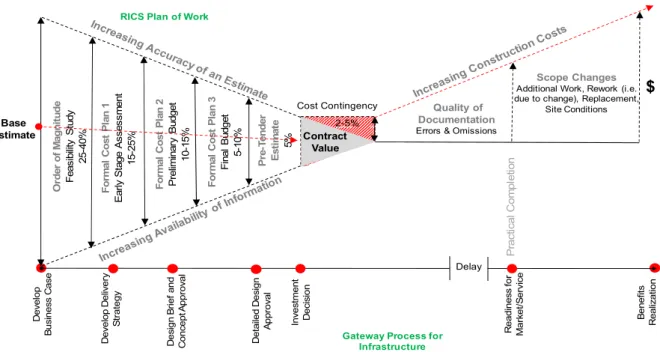
change-orders, which can lead to cost increases being incurred (Allen Consulting and the University of Melbourne, 2007). With this in mind, it is suggested that it is misleading to make direct comparisons between the base estimate at the time of the decision-to-build and actual construction costs, as the estimate that is initially prepared is typically based upon a conceptual design. As noted in Figure 1, the accuracy of an estimate improves as more information becomes available (e.g., scope is defined and users’ requirements are identified). In Figure 1, Ashworth’s (2008) percentage range for each type of estimate that is produced during the design development phase of a project is presented (p.251).

Figure 1. Traditional cost scenario for infrastructure projects

At this juncture, it is important to mention that the Royal Institution of Chartered Surveyors (RICS) under the auspices of the ‘New Rules of Measurement’ advocate that all estimates are expressed as a single figure (RICS, 2012). The use of such a precise figure is failing the basic tests of validity:

O rde r of M agni tu de F ea sib ility S tu dy 25-40 % F o rm al C o st P lan 1 E ar ly S ta ge A sse ssm en t 15 -2 5% F o rm al C o st P lan 2 P rel im in ar y B udg et 10 -1 5% For m al C o st Pl an 3 F ina l B udg et 5-10 % P re -T ender Es ti m at e 5% Cost Contingency 2-5% Scope Changes Additional Work, Rework (i.e. due to change), Replacement,

Site Conditions Quality of

Documentation Errors & Omissions Base Estimate Contract Value $ De ve lo p B u si n e ss C a se De ve lo p De liv e ry S tr a tegy D e si gn B rie f a nd C o nc ep t A ppr o val D e ta ile d D e si g n A p pr o val In ve st me n t D e ci si o n R e ad in es s f o r Ma rk e t/ S e rv ice P ra cti ca l C o m p le tio n B e n e fits R e a liz a tio n

Gateway Process for Infrastructure RICS Plan of Work

accuracy and precision (Newton, 2012). The inadequacies of the traditional estimating process are camouflaged by the use of deterministic percentage additions that take the form of a contingency, which cater for an increase in a project’s cost due to: (1) variability (i.e. random uncertainty); (2) risk events; and (3) unforeseeable situations (Baccarini and Love, 2014). In stark contrast to the deterministic approach, it has been suggested the application of a probabilistic approach to determining a construction cost contingency based upon empirical analysis of a wide range of infrastructure projects should be applied (e.g. Baccarini and Love, 2014).

Generally, the construction contingency percentages applied to public infrastructure projects have been unable to accommodate increases in cost that are incurred. For example, Baccarini and Love (2014) analysis of 228 water infrastructure projects revealed that the mean percentage addition was 8.46% of their contract value, but the construction contingency requirement for the final cost was 13.58%; a shortfall in contingency in the region of 5%. The magnitude of this percentage addition, while evidently inaccurate, can vary with the nature of the project and the type of procurement method adopted. For example, in the case of a greenfield project that is being delivered via a traditional procurement method (e.g., Construct Only), the design and specifications (including drawings and Bills of Quantities (BoQ)) for a project are supposed to be complete at the award of a tender and thus a construction contingency between 2% and 5% is often provided. As a result, there is a perception that a high degree of cost certainty will ensue, but in reality this is fallacy, as complete drawings and BoQs are seldom available when a project goes to tender. As previously mentioned, they invariably contain errors and omissions, which can lead to change-orders and rework and increased construction costs (Love et al., 2012).

Brownfield projects can be considered to be higher risk ventures than greenfield sites (e.g., due to geotechnical uncertainties, contaminated soil and neighboring structures). Thus, in the case of Brownfields projects, a public sector client may opt to use a non-traditional procurement route (e.g. Design and Construct) and transfer the associated risks for the development to a single-entity as well as be provided with a Guaranteed Maximum Price, for the works. Any changes in the scope of work under this form of contractual arrangement, however, will require a client to pay a premium for any changes that are required. It is, therefore, necessary to have a sufficient contingency allowance in place should the need for amendments arise (De Marco et al., 2015).

Explanations for Deviations in Cost Performance

The literature is replete with explanations as to ‘how’ and ‘why’ the cost performance of public sector infrastructure projects deviates from their expected outturn cost (e.g., Pickrell, 1992; Bordat et al. 2004; Odeck, 2004; Siemiatycki, 2009; Odeck et al., 2015). According to Love et al. (2016) two schools of thought have emerged explaining deviations in the cost performance of infrastructure projects: (1) ‘Evolution Theorists’, who have suggested that cost deviations materialize as a result of changes in scope and definition between a project’s inception and completion. The Office of the Auditor General in Western Australia (2012), for example, revealed that changes in scope were the primary culprit that had contributed to cost overruns occurring in their major capital projects. Next are (2) ‘Psycho Strategists’ who have advocated that projects experience cost overruns due to deception, planning fallacy and unjustifiable optimism bias in establishing the initial cost targets (Flyvbjerg et al. 2002; Siemiatycki, 2009). According to Flyvbjerg (2003) those responsible for determining the budget for an infrastructure project are often subjected to applying Machiavelli’s formula to ensure it is given approval to proceed: costs

are underestimated (-), revenues are over estimated (+), environmental impacts undervalued (-) and development effects are overvalued (+) (p.43).

Often estimators/planners only consider the information that is made available to them for the particular project they are involved with delivering; such a focus is referred to as having an ‘inside view’ (Flyvbjerg et al., 2005). In particular, Kahneman and Lovallo (1993) observed that “the inside view is overwhelmingly preferred in intuitive forecasting. The natural way to think about a problem is to bring to bear all one knows about it, with special attention to its unique features” (p.26). Contrastingly, an ‘outside view’ recognizes that projects of a similar nature should be used as a reference point when assessing a project (Kahneman and Lovallo, 1993). By adopting an ‘outside view’ Flyvbjerg (2008) suggests that a more realistic forecast of cost can be acquired and thereby reduce the propensity for optimism bias to arise.

In theory, the proposition that has been proposed by Flyvbjerg (2008) is plausible, however, in practice a different reality exists (Love et al., 2016). For example, Perth Arena’s initial budget estimate was established based on square meter rate with reference to Melbourne Park’s Multi-Purpose Venue (formerly known as Vodafone Stadium and with a construction cost of AU$65 million in 2000). The initial estimate was AU$165 million, which then increased to AU$343 within two years, and with a final completion cost in excess of AU$550 million (Office of the Auditor General, 2010). According to Love et al. (2016) both ‘inside’ and ‘outside’ views need to be adopted to adequately explain the causal nature of cost overruns. However, the research presented in this paper does not seek to explain ‘why’, but bring to the fore ‘how’ cost overruns occur by illustrating the direct financial consequences of poorly managed public infrastructure projects. At

the time a project’s contract is signed, cost certainty should be affirmed, unless a form of cost-plus agreement is otherwise agreed.

Illustrative Case Study

Most research studies that have examined the cost performance of infrastructure projects have tended to rely upon heterogeneous datasets (e.g., Flyvbjerg et al., 2002; Cantarelli et al., 2012). Such datasets are loosely connected and thus there is a propensity for them to possess a considerable amount of ‘noise’, as a morass of missing information is adequately needed to explain the nature of a project’s cost performance (e.g. by way of an asset owners’ aims and objectives, planning requirements, contractors, project teams, technologies, and contractual arrangements). Instead, this research sought to obtain an ameliorated understanding of the impact of change-orders on the public sector and contractors financial performance.

To illustrate how the cost performance of infrastructure projects varies and provide an insight to the problem that confronts the public sector, a case study is used (Fry et al., 1999). Typically, an illustrative case study is used to describe an event; they utilize one or two instances to demonstrate the reality of a situation (e.g., change-orders and margin). In this instance, the case study provides a platform to demonstrate that the cost performance of public sector projects has been mismanaged. The case study serves to make the ‘unfamiliar, familiar’, and provide a common language for the nature of infrastructure projects’ cost performance. A homogenous dataset (i.e. in terms of processes, technologies, procedures and processes) from a contractor who completed a wide range of infrastructure projects between 2011 to 2014 are examined where their final accounts had been completed; that is, the final payment made to the contractor on completion of the works described

in the contract and payments owing being made at the end of the defects liability period (typically, 6-12 months after handover). Selecting only those projects that had their final accounts completed enabled an accurate assessment of their cost to be determined. No project sampled was subjected to open tendering, and several were delivered within a Building Information Modelling (BIM) environment. Individual names, locations, and the Level of Development (LOD) specification of projects are withheld and the data aggregated for reasons of commercial confidentially.

Analysis and Findings

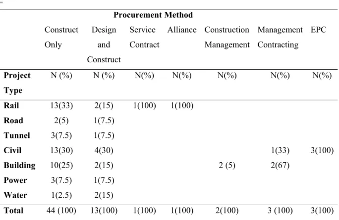
Cost data from 67 completed infrastructure projects were provided, which included their procurement method, original contract value (OCV), final contract value, contractor’s margin, total of client approved change-orders, and final contractor’s margin. Table 1 provides a summary of the types and procurement methods for the 67 infrastructure projects that were constructed throughout Australia within the study period (Table 1). ‘Building’ (n=16, 24%) (e.g., hospitals, schools and civic assets) and ‘Rail’ (n=16, 24%) and ‘Civil’ (n=22, 33%) (i.e., miscellaneous works such as dam upgrades and earthworks) were the most popular types of projects that were constructed. A variety of procurement methods were selected by the public sector to deliver their assets (Table 1); 65 (44%) were traditional ‘Construct Only’ lump sum contracts and the remainder being non-traditional methods with the most popular form being ‘Design and Construct’, (n=13,19%). Tables 2 and 3 provide an overview of the cost performance parameters of projects and a breakdown by their type, respectively.

Table 1. Projects and procurement methods = Procurement Method Construct Only Design and Construct Service Contract Alliance Construction Management Management Contracting EPC Project Type N (%) N (%) N(%) N(%) N(%) N(%) N(%) Rail 13(33) 2(15) 1(100) 1(100) Road 2(5) 1(7.5) Tunnel 3(7.5) 1(7.5) Civil 13(30) 4(30) 1(33) 3(100) Building 10(25) 2(15) 2 (5) 2(67) Power 3(7.5) 1(7.5) Water 1(2.5) 2(15) Total 44 (100) 13(100) 1(100) 1(100) 2(100) 3 (100) 3(100)

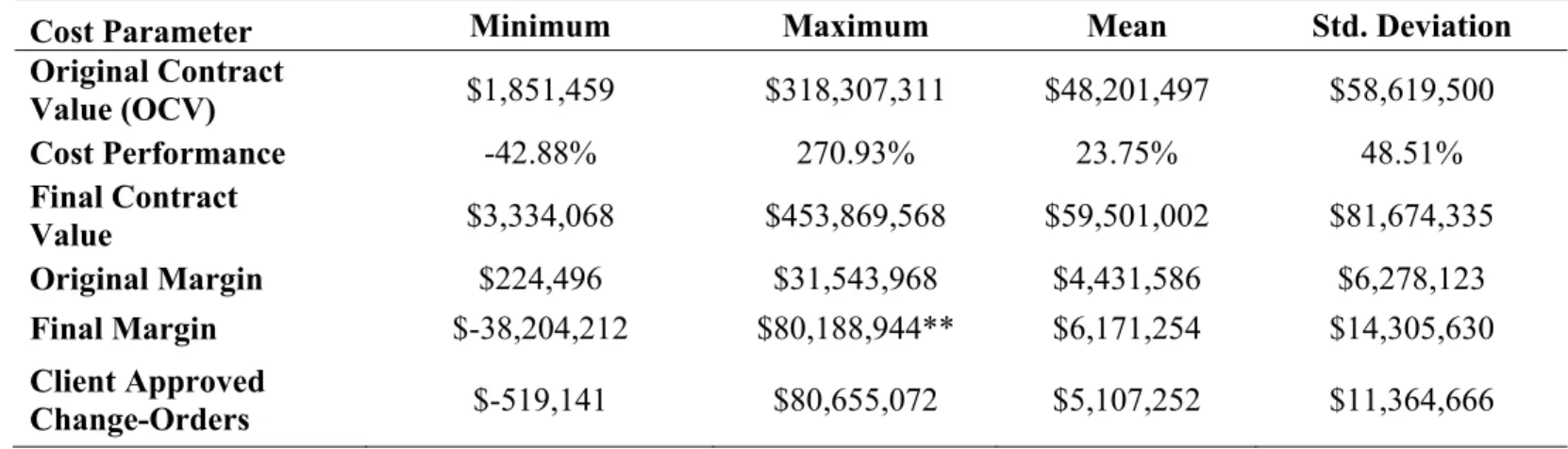
Table 2. Descriptive statistics for cost performance parameters

Cost Parameter Minimum Maximum Mean Std. Deviation Original Contract Value (OCV) $1,851,459 $318,307,311 $48,201,497 $58,619,500 Cost Performance -42.88% 270.93% 23.75% 48.51% Final Contract Value $3,334,068 $453,869,568 $59,501,002 $81,674,335 Original Margin $224,496 $31,543,968 $4,431,586 $6,278,123 Final Margin $-38,204,212 $80,188,944** $6,171,254 $14,305,630 Client Approved Change-Orders $-519,141 $80,655,072 $5,107,252 $11,364,666

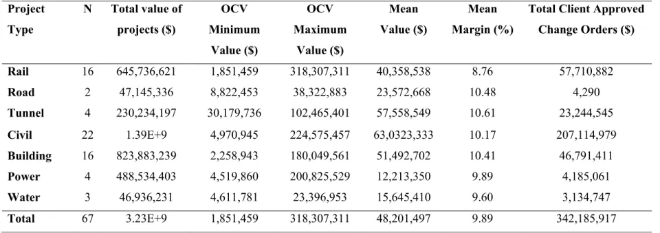
Table 3. Original contract values and approved change orders Project Type N Total value of projects ($) OCV Minimum Value ($) OCV Maximum Value ($) Mean Value ($) Mean Margin (%)

Total Client Approved Change Orders ($) Rail 16 645,736,621 1,851,459 318,307,311 40,358,538 8.76 57,710,882 Road 2 47,145,336 8,822,453 38,322,883 23,572,668 10.48 4,290 Tunnel 4 230,234,197 30,179,736 102,465,401 57,558,549 10.61 23,244,545 Civil 22 1.39E+9 4,970,945 224,575,457 63,0323,333 10.17 207,114,979 Building 16 823,883,239 2,258,943 180,049,561 51,492,702 10.41 46,791,411 Power 4 488,534,403 4,519,860 200,825,529 12,213,350 9.89 4,185,061 Water 3 46,936,231 4,611,781 23,396,953 15,645,410 9.60 3,134,747 Total 67 3.23E+9 1,851,459 318,307,311 48,201,497 9.89 342,185,917

Cost Performance

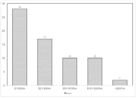
The value of the contracts that had been awarded by the public sector varied, though a significant proportion were less than AU$100 million (n=55, 82%) as denoted in Figure 2. The contract value of the projects ranged from approximately AU$1.8 million to AU$318 million, with a mean of AU$48 million (Table 2). More specifically, ‘Civil’, (43%) ‘Building’ (25%) and ‘Rail’ (20%) project types accounted for a majority of the contractor’s turnover from 2011 to 2014 (Table 3).

Figure 2. Number of infrastructure projects

It can be seen that the cost performance of projects ranged from -42.88% to + 270.93% of budget with a mean cost overrun of 23.75% as a proportion of the OCV. This finding is in stark contrast to Love (2002) who reported a mean cost overrun of 12.6% of the OCV, with 48% being attributable to change-orders and the remaining 52% being due to rework. All projects that utilized BIM to a minimum of LOD 300 experienced cost increases; in this instance, specific model elements are demonstrated as specific assemblies accurate in terms of quantity, size, shape, location and orientation.

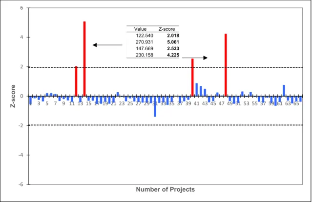
A total of 67% (n=45) of projects incurred a cost overrun of less than 25% of the OCV and 9% (n=6) experienced a cost underrun. A Grubbs test was used to detect outliers from a Normal Distribution with the tested data being the minimum and maximum values (Grubbs, 1950). The result is a probability that belongs to the core population being examined. So, if the data is approximately normally distributed, then outliers are required to have Z-scores ± 3. Outliers possessing a Z-score in the range ± 2 to 3 can be considered to be ‘borderline’ outliers. As denoted in Figure 3, two projects were identified as being ‘borderline’ with Z-scores being between +2 and +3 and two outright outliers being in excess of +4. Considering these Z-scores, the ‘best fit’ distribution was determined. Considering the outliers that were present, a Normal Distribution was not deemed to be the ‘best fit’ distribution’ for the data.

Figure 3. Determination of outliers for cost performance

-6 -4 -2 0 2 4 6 1 3 5 7 9 11 13 15 17 19 21 23 25 27 29 31 33 35 37 39 41 43 45 47 49 51 53 55 57 59 61 63 65 Z-s co re Number of Projects Value Z-score 122.540 2.018 270.931 5.061 147.669 2.533 230.158 4.225

The ‘best fit’ probability distribution for ‘cost performance’ was examined so that probability of cost deviations (i.e., underruns and overrun) could be determined at the point of contract award (Love et al., 2013); the computation of such a distribution is both pertinent to the public sector and contractors as part of formulating a risk management strategy for their projects.A caveat, however, needs to be made here; the data’s homogeneity would likely provide a more accurate assessment of risk for the contractor, but could provide public sector clients with ‘ballpark’ probabilities to formulate future construction contingencies. ‘Underruns’ and ‘overruns’ should be separated when examining cost performance, but considering the limited number of projects that were below the agreed contract value it was decided to combine them together in this case.

Using the ‘Goodness of Fit’ Kolmogorov-Smirnov (D), and Anderson-Darling (A2_{) tests it was} revealed that Generalized Extreme Value (GEV) distribution with parameters k = 0.51, σ = 11.98,

μ = 4.43 was identified as the ‘best fit’ solution for examining the cost performance for the sample of projects. The Kolmogorov-Smirnov (K-S) test revealed a D statistic of 0.13 with a P-value of 0.17. The Anderson-Darling (A-D) statistic A2 _{was revealed to be 5.21. The K-S test accepted the} Null Hypothesis (i.e., H0 where it is assumed that there is no difference in parameters) for the sample distribution’s ‘best fit’ at the critical nominated α values of 0.2, and at 0.01 for the A-D test. The resulting GEV probability density function (PDF) is expressed as:

( ) = exp (−(1 + ) )(1 + ) ≠ 0

where z=(x-μ)/σ, and k, σ, μ are the shape, scale, and location parameters respectively. The scale must be positive (sigma>0), the shape and location can take on any real value. However, the range of definition for the GEV distribution depends on k:

1 + ( − )> 0 ≠ 0 −∞ < < +∞ = 0

[Eq.2]

Using the GEV PDF the probability of cost overrun of 23.75% is 73% (P=0.73). The proportion of projects (67%) that experienced less than 25% cost overrun had a mean of 7.9%; the probability a project exceeds its OCV is 0.58%.

The detailed financial summaries provided to the researchers by the contractor revealed that client change-orders contributed to the cost deviations that were subjected to public sector clients’ approval. Non-conformances also materialized in the projects, but the rectification costs did not impact the final contract value paid by the clients as these were the responsibility of the subcontractors and suppliers.

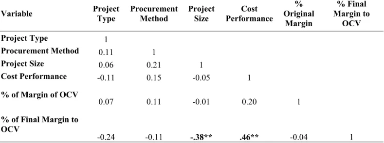
The correlation analysis presented in Table 4 reveals that the size of a project in terms of its OCV, its type, and the procurement method used were not significantly related with cost performance (p <0.01). Studies examining the relationship between project size and the extent of cost overrun that is incurred remains inconclusive and has been the subject of debate (e.g., Odeck, 2004; Love et al., 2013). In pursuing this unresolved issue, the analysis sought to determine if there was a

Table 4. Correlations between project characteristics and cost measures

Variable Project _Type Procurement _Method Project _{Size Performance} Cost

% Original Margin % Final Margin to OCV Project Type ₁ Procurement Method _{0.11 1} Project Size _{0.06 0.21 1} Cost Performance _{-0.11 0.15 -0.05 1} % of Margin of OCV 0.07 0.11 -0.01 0.20 1 % of Final Margin to OCV -0.24 -0.11 -.38** .46** -0.04 1

A one-way Analysis of the Variance (ANOVA) was used in this instance to test for differences. Levene’s test for homogeneity of variances was not found to be violated (p <0.05), which indicates the population variances for project size and cost performance were equal. Thus, there were no significant differences between ‘project size’ and cost performance, F (4,62) = 1.096, p <0.05). Furthermore, to determine whether there was a difference between procurement methods and cost performance, a t-test was undertaken using the categories of ‘traditional’ and ‘non-traditional’.

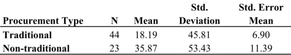
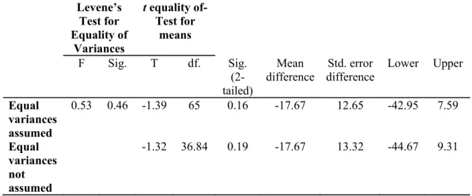
Table 5 presents the mean and standard deviation for the cost performances for categorized procurement types, and the results of the t-test are presented in Table 6. At the 95% confidence interval, no significant difference in cost performance was experienced in projects delivered under the different procurement categorizations that were established. Akin with previous research it can be concluded that cost performance does not significantly vary with the procurement methods employed (e.g., Love, 2002).

Table 5. Cost performance for procurement types

Procurement Type N Mean

Std. Deviation Std. Error Mean Traditional 44 18.19 45.81 6.90 Non-traditional 23 35.87 53.43 11.39

Table 6. t-test for difference between cost performance and procurement types Levene’s Test for Equality of Variances t equality of-Test for means F Sig. T df. Sig. (2-tailed) Mean difference Std. error difference Lower Upper Equal variances assumed 0.53 0.46 -1.39 65 0.16 -17.67 12.65 -42.95 7.59 Equal variances not assumed -1.32 36.84 0.19 -17.67 13.32 -44.67 9.31 Change-Orders

The mean amount of client approved change-orders that occurred in projects was approximately AU$5.1 million (10.6%) (Table 2). In addition, the total change-orders accounted for 11% of the value of the work that was undertaken by the contractor between 2011 and 2014 (Table 3). To determine if there was a significant difference between the change-orders and project size an ANOVA was undertaken. Levene’s test for homogeneity of variances was found to be violated (p = 0.00), which indicates the population variances for project size and cost performance were not equal. Significant differences between change-orders and project size were found to occur, F (4,62) = 5.525, p <0.01). A Tukey’s HSD post-hoc tested showed that projects with lower a OCV experienced smaller volumes of change-orders (p <0.05).

Margin

According to the NAO (2013) there is limited available knowledge and a lack of transparency surrounding the margins of contractors. In contributing to this gap in knowledge, the analysis revealed that the contractor’s mean margin (excluding overheads) was 9.89% of the OCV. Table 3 provides a breakdown of the mean margin allocated for each type of project, which ranged from 8.76% to 10.61%.

The lowest record margin was 3.98% of the OCV for a ‘Civil’ project that had an OCV of AU$48.4 million and a final contract value of AU$65.9 million. However, in this project the contractor’s expected margin at the commencement of the works was AU$3.8 million, but declined to AU$3.2 million (-15.57%) due to issues surrounding rework, which they were accountable for. This scenario was observed in several projects, for example, an AU$64.7 million ‘Construct Only’ ‘Civil’ project that had an expected margin of AU$2.9 million. With the client issuing scope changes, the final contract value was AU$61.6 million, a cost underrun of 4.06%. The contractor experienced a staggering loss of AU$38.2 million, which occurred due to an array of issues that included rework, product non-conformances and delays to works (Table 2). Disastrous projects of this nature can, and more often than not, usually result in contractors being liquidated. If, however, as in this case, they are able to shoulder such costs, then their stock value, reputation and image within the public and private sectors and the general community can be adversely impacted. Losses in one project can be offset against gains in others that form part of a contractor’s portfolio of work in progress. For example, the maximum recorded final margin as noted in Table 2 was AU$80.18 million for a project that had an OCV in excess of AU$1 billion and incurred a cost increase of 7.5%.

The project that had the highest margin (> 30%) was a ‘Building’ project with an OCV of AU$3.38 million, which increased by 25.76% in value to AU$4.87 million due to change-orders. In contrast to the aforementioned example, this project’s margin increased from an expected value of AU$641,608 to AU$1.37 million (114.33%). Surprisingly, the projects with margins in excess of 20% of their OCV varied in size, type, and location. Figure 4 identifies three ‘borderline’ and two ‘outlier’ projects that possessed high margins. For example, a ‘Civil’ project had an OCV of $138 million with a margin of 22.82%. Conversely, a ‘Building’ project had an OCV of AU$2.5 million with a margin of 28.98%.

Figure 4. Determination of outliers for margin

-5 -4 -3 -2 -1 0 1 2 3 4 5 1 3 5 7 9 11 13 15 17 19 21 23 25 27 29 31 33 35 37 39 41 43 45 47 49 51 53 55 57 59 61 63 65 Z -score Number of Projects Value Z-score 26.411 2.868 22.824 2.238 26.616 2.904 28.978 3.318 32.327 3.907

Considering the prevailing ‘outliers’ the ‘best fit’ distribution was computed, and can ceteris paribus be used to determine the likelihood of a contractor’s margin by the public sector. As above, the K-S and A-D ‘Goodness of Fit’ tests were undertaken. The results of the ‘Goodness of Fit’ tests revealed that the Wakeby distribution provided the ‘best fit’ for the dataset. The K-S test revealed a D-statistic of 0.07573 with a P-value of 0.80413 and the A-D statistic A2 _{was revealed}

to be 0.47668 at the critical nominated α values of 0.01. The Wakeby is a form of GEV distribution. The parameters of a Wakeby, α β γ δ ξ are all continuous. The domain for this distribution is expressed as , if and , if or . The distribution parameters for the range were α = 21.367, β = 4.5569, γ = 1.71, δ =0.45437, ξ=3.0078. The Wakeby distribution is defined by the quantile function (i.e. inverse CDF):

[Eq.3]

The Wakeby PDF is used to determine the likelihood of a mean of 9.89% margin if applied to a project; in this instance, there is a 62% (P=0.62) probability that this margin would be applied.

The mean margin OCV contract award for various sizes of projects can be seen in Table 7. It can be seen the mean margins do not significantly vary between one and another rendering the Wakeby distribution identified above as a basis for determining the likely margin that would be applied. Levene’s test for homogeneity of variances confirms this observation as it was not found to be violated (p <0.05), which indicates the population variances for project size and margin are equal. Thus, there were no significant differences between ‘project size’ and margin, F (4,62) = 3.04., p

x ≤ ξ δ ≥ γ >0 ξ≤x≤+α β−γ δ _{δ <}0 γ =0

(

)

(

)

(

(

)

)

<0.05). A significant association, however, was found to be present with the percentage increase of the final margin with project size, r=-038, n=67, p < 0.01, two tails and cost performance and r=-046, n=67, p < 0.01, two tails. It can be therefore implied that the likelihood of an increase in expected margin at contract decreases with smaller OCVs. In addition, the margins of a contractor increase as a project experiences larger cost overruns.

To determine whether there was a difference between procurement methods and margin, a t-test was undertaken using the categories of ‘traditional’ and ‘non-traditional’. Table 8 presents the mean and standard deviation for the cost performances for categorized procurement types, and the results of the t-test are presented in Table 9. At the 95% confidence interval, no significant difference in margins was determined under the different procurement categorizations that were established.

Table 7. Size and margin % of contract value

Project Size N Mean (%) Minimum (%) Maximum (%) Std. Deviation $1-$20m 28 10.26 3.98 32.33 6.15 $21-$50m 17 8.54 0.00 26.41 5.79 $51-$100m 10 10.60 4.01 26.62 6.69 $101-$200m 10 10.32 6.17 22.82 4.81 >$201m 2 9.91 9.91 10.04 0.91 Total 67 9.89 0.00 32.33 5.79

Table 8. Margin for procurement types

Procurement Type N Mean

Std. Deviation Std. Error Mean Traditional 44 9.56 5.50 0.82 Non-traditional 23 10.61 6.52 1.39

Table 9. t-test for difference between contractor’s margin and procurement types

Levene’s Test for Equality of Variances t equality of-Test for means F Sig. T df. Sig. (2-tailed) Mean difference Std. error difference Lower Upper Equal variances assumed 0.32 0.56 -0.68 65 0.49 -1.04 1.52 -4.09 2.01 Equal variances not assumed -0.64 36.31 0.52 -1.04 1.62 -4.32 2.24

The dominant paradigm within the public sector assumes that differing procurement options can provide varying degrees of cost certainty and will influence the level of a contractor’s margin, which is a reflection of their risk profile; the findings presented from this illustrative case study suggest the contrary, and provide a basis for the public sector to better understand the unintended consequences of change-orders that can arise during the delivery of their assets. The level of a contractor’s margin is a small component of their cost, yet having an understanding of this amount is important, as the balance of risk and reward can distort their behavior if they are not aligned

(Love et al., 2011). Thus, the balance of risk and reward is dependent upon the structure of the contract and how well it is managed (NAO, 2013).

Discussion

What matters most to the taxpayer is whether contracted out services can provide improved quality at an appropriate overall cost (NAO, 2013: p.15). Taxpayers concerns, however, are not being adequately addressed; evidence of this can be seen with the sheer number of public sector projects that have and continue to experience cost overruns. This is not to say that the public sector is neglecting such concerns; quite the contrary, as it is acknowledged that significant effort has been undertaken to redress the issues that adversely impact the delivery of infrastructure projects. After all public-sector employees are also taxpayers and therefore there should be a resounding motivation for them to ensure assets and services are delivered, operated and maintained cost effectively. However, despite noble intentions, there is a residing suspicion that spending other peoples’ money on other people absolves them from any form of accountability, which often results in assets not providing the VfM that was initially intended. This case in point was originally highlighted by Milton Friedman (2004) who perceptively stated: “I can spend somebody else's money on somebody else. And if I spend somebody else's money on somebody else, I'm not concerned about how much it is, and I'm not concerned about what I get. And that's government”.

The magnitude of change-orders that occurs in projects is troublesome and hinders public sector ability to cost effectively ensure the asset being delivered is ‘future proofed’; that is, resilient to unexpected events and adaptable to changing needs, uses or capacities. Changes during construction may lead to sub-optimal solutions (e.g., design, functionality, materials, running

costs) being incorporated into an asset’s fabric to minimize cost and meet the committed completion date.

Irrespective of the procurement strategy adopted, change-orders were found to materialize during construction. An analysis of the nature of change-orders is outside the remit of this paper, but it was observed that changes in scope, and errors and omissions in documentation predominated. Such levels of change indicate that the ‘design’ process has not been effectively managed, irrespective of the procurement option, and the use of BIM, though as noted this was only used in a limited number of projects. The authors did not have access to the construction contingency of the public-sector clients, but a deterministic figure between 2% and 5% (Baccarini and Love 2014), which is often applied would have obviously been inadequate for the sampled projects. Prior to the commencement of construction, a contingency in excess of this value would be unacceptable for the public sector, as there is unequivocally a need for cost certainty. But, there remains the ‘elephant in the room’, with no party wanting to be held accountable for contributing to the development and production of an incomplete scope and poor quality tender documentation. Naturally, contractors will submit a bid based upon the information that they have been provided and may opportunistically price items within the BoQ where they anticipate future changes to materialize to maximize their margin.

In light of the status quo, cost overruns due to change-orders will continue to prevail and could even be exacerbated as there is a misconception that digitization of the design process enabled by the use of BIM will reduce errors and omissions. Simply superimposing a 21st _{century innovation} such asBIM to procurement practices where contracts do not wholly support collaborative working

and have been essentially developed for the 20th _{century, will not leverage the benefits that can be} afforded from its adoption. Thus, to mitigate change-orders, behavioral, cultural, legal and structural issues associated with the delivery of public sector assets need to be transformed to effectively accommodate the benefits that can be afforded by BIM, especially if they are to be future-proofed. The inclusion of contractors and asset managers in the design process is needed to help reduce changes using visualization and enable future-proofing to take place (Figure 5). This can be done by ensuring the information needed to effectively operate and maintain an asset is captured and provided in a usable format that is readily accessible (Figure 6).

(a) A 3D visualization of what is to be constructed (b) Actually constructed

Figure 6. Centralization of asset information for operations and maintenance

Considerable effort has been and continues to be made to address the aforementioned issues to support the digitization of assets throughout their life-cycle, particularly in the United Kingdom (e.g. Construction Industry Council, 2014). While such efforts provide the building blocks for enabling the much-needed transformational change, many public-sector agencies are still ‘sitting on the fence’ with regard to rolling out BIM and implementing the new procurement practices that are required, despite being cognizant of the problems associated with existing approaches of asset delivery. Indeed, this is a bold proposition, however, if the public sector is to make headway in ensuring that assets are delivered cost effectively, then a charter focusing on procurement reform needs to be initiated, managed and maintained; changes initiated in the past have been ephemeral.

Conclusion

Public infrastructure projects that experience cost overruns adversely impact taxpayers. It is therefore imperative that they are not only delivered within budget but also continue to be of value into the future. Providing infrastructure that is resilient and adaptable to changing needs, capacities and uses should be the ultimate goal of the public sector. The path to attaining this goal can be derailed when change-orders (e.g., in scope) are required during construction, and can lead to sub-optimal assets being delivered. The taxpayer pays for this additional cost, while contractors are rewarded with an increase in their margins; this is the ‘elephant in the room’ within the public sector, which is underpinned by ‘spending somebody else's money on somebody else’.

In examining the cost performance of public infrastructure projects an illustrative case study was undertaken. Cost information from 67 projects constructed between 2011 and 2014 were provided by a contracting organization. The cost overruns/underruns that were experienced were calculated from the contract award to when final accounts were completed. The analysis revealed that the cost performance of projects ranged from -42.88% to + 270.93%, with a mean cost overrun of 23.75%. and a probability of occurring of 73%.In alignment with previous research no significant differences in the magnitude of cost overruns were found to exist by a project’s contract value, types, and procurement method. It revealed that change-orders accounted for a significant proportion of the cost overruns that emerged in the projects, with a mean of 10.6% as a proportion of the original contract value. Notably, significant differences were found to occur between a project’s size and change-orders; that is, those with a smaller original contract value experienced a smaller volume of change-orders.

Limited knowledge has existed about the margins that contractors apply to projects. However, the mean margin applied to the sample of public sector projects was revealed to be 9.89%, and the likelihood of such a value being applied was computed to be 62%. The analysis revealed that the margin applied by the contractor did not vary with project type, its size and the procurement method being used to construct the asset. The analysis also demonstrated a positive association with an increase in change-orders and the contractor’s margin. More specifically it was found that contractor’s margins increase with larger cost overruns. A significant proportion of the projects were delivered using traditional ‘Construct Only’ and there is no incentive for contractors reduce change-orders as they have had no involvement in the design process. Even when the contractor was involved in the design process, change-orders still occurred, though their extent was unable to be determined.

Involving the contractor as early as possible in the design process, providing incentives, and open-book tendering are considerations that should be enacted as initial steps to mitigate change-orders. As the public sector embraces the era of digitization, which is being enabled by Building Information Modelling, the need to integrate design and construction and engender collaboration is imperative to ensure assets can be delivered cost effectively and future-proofed. Emphasis here should not necessarily be placed on the technology but ensuring information is structured in a standardized format, captured, openly-shared, stored and accessible so that parties can effectively work in a collaborative environment. The research in this paper provides invaluable empirical evidence, though based on a limited dataset of 67 projects, to support the need for a change to the way the public sector procures their assets. If change is not embraced, then cost overruns will continue to be a nemesis.

References

Allen Consulting and The University of Melbourne (2007). Performance of PPPs and Traditional Procurement in Australia. Final Report for Infrastructure Australia, November, (Available at: http://www.infrastructure.org.au/content/ppp.aspx, Accessed 23rd December 2016)

Ashworth, A. (2008). Pre-contract Studies: Development Economics, Tendering and Estimating. Third Edition, Blackwell Publishing, Oxford, UK

Baccarini, D., and Love, P.E.D. (2014). Statistical characteristics of contingency in water infrastructure projects. ASCE Journal of Construction Engineering and Management,

140(3), 04013063.

Bordat, C.B., McCulloch, K.C., Sinha, K.C., and Labi, S. (2004). An Analysis of Cost Overruns and Time Delays of INDOT Projects. In: Publication FHUW/INTRP-2007.04, Joint Transportation Research Program, Indiana Department of Transport and Purdue University, West Lafayette, Indiana, USA.

Cantarelli, C., Flyvbjerg, B. and Buhl, S.L. (2012). Geographical variation in project cost performance: the Netherlands versus worldwide. Journal of Transport Geography, 24, pp. 324–331

De Marco, A., Rafele, C., and Thaheem, M. (2015). Dynamic management of risk contingency in complex design-build projects. ASCE Journal of Construction Engineering and Management, 142(2),10.1061/(ASCE)CO.1943-7862.0001052, 04015080.

Friedman, M. (2004). ‘Your World’ interview with economist Milton Friedman Available at:

http://www.foxnews.com/story/2006/11/16/your-world-interview-with-economist-milton-friedman.html , Accessed 16th December

Fry, H., Ketteridge, S., and Marshall S. (1999). A Handbook for Teaching and Learning in Higher Education, Glasgow, Kogan Page, pp.408

Flyvbjerg, B., Holm, M.K., and Buhl, S. (2002). Underestimating costs in public works: Error or lie. Journal of the American Planning Association, 68(3), pp.279-295.

Flyvbjerg, B. (2003). Machiavellian tunnelling. World Tunnelling, Available at

http://flyvbjerg.plan.aau.dk/WorldTunnelling.pdf, Accessed 23rd _{December 2016}

Flyvbjerg, B. (2008). Curbing optimism bias and strategic misrepresentation in planning: reference class forecasting in practice. European Planning Studies, 16(1), pp.3-21.

Grubbs, F.E. (1950). Sample criteria for testing outlying observations. Annals of Mathematical Statistics. 21(1), pp.27–58

Jarkas, A.M. (2014). Factors impacting design documents quality of construction projects. International Journal of Design Engineering, 5(4), pp.323-343

Kahneman, D. and Lovallo, D. (1993). Timid choices and bold forecasts: A Cognitive perspective on risk taking. Management Science39(1), pp.17-31.

Love, P.E.D. (2002). Influence of project type and procurement method on rework costs in building construction projects. ASCE Journal of Construction Engineering and Management128(1) pp. 18-29.

Love, P.E.D, Edwards, D.J., and Irani, Z. (2012b). Moving beyond optimism bias and strategic misrepresentation: An explanation for social infrastructure project cost overruns. IEEE Transactions on Engineering Management 59(4), pp. 560 – 571.

Love, P.E.D., Sing, C-P., Wang, X., and Tiong, R. (2013). Determining the probability of cost overruns in Australian construction and engineering projects. ASCE Journal of Construction Engineering and Management, 139(3), pp. 321–330.

Love, P.E.D., Simpson, I., Olatunji, O. Smith, J. and Regan, M. (2015a). Understanding the landscape of overruns in transportation infrastructure projects. Environment and Planning B: Planning and Design, 42(3), pp. 490 – 509.

Love, P.E.D., Sing, C-P., Carey, B. and Kim, J-T. (2015b). Estimating construction contingency: Accommodating the potential for cost overruns in road construction projects ASCE Journal of Infrastructure Systems, 21(2) 04014035.

Love, P.E.D. Ahiaga-Dagbui, D.D., and Irani, Z. (2016). Cost overruns in transportation infrastructure projects: Sowing the seeds for a probabilistic theory of causation. Transportation Research A: Policy and Practice, 92, pp.184-194.

Love, P.E.D., Zhou, J. Iran, Z., Edwards, D.J. and Sing, C.P. (2017a). Off the rails: Cost performance of rail infrastructure projects. Transportation Research Part A: Policy and Practice, 99, pp.14-29

Love P.E.D. Ahiaga-Dagbui, D., Welde, M., and Odeck, J. (2017b). Cost performance light transit rail: Enablers of future-proofing. Transportation Research A: Policy and Practice, 100, pp.27-39.

NAO (2013). Government Contracting: The Role of Major Contractors in the Delivery of Public Services. Memorandum for Parliament, National Audit Office (NAO), HC-810, Session 2013-2105, 12th _{November, The Stationary Office, London, United Kingdom}

Newton, S. (2012). Improving a cost estimate using reference class analytics. In Proceedings United Kingdom: Birmingham School of the Built Environment, Birmingham City University, UK, pp. 73-83. Available at: http://www.irbnet.de/daten/iconda/CIB_DC25600.pdf, Accessed 28th _September

2016

Odeck, J. (2004). Cost overruns in road construction – what are their size and determinants. Transport Policy, 24, pp.43-53.

Odeck, James. (2014) Do reforms reduce the magnitudes of cost overruns in road projects? Statistical evidence from Norway. Transportation Research Part A: Policy and Practice.

Odeck, J. Welde, M., and Volden, G.H. (2015). The impact of external quality assurance of cost estimates: empirical evidence from the Norwegian road sector. European Journal of Transportation Infrastructure Research, 10, pp.77-88.

Office of the Auditor General (2010). Western Australian Auditor General’s Report: The Management of Perth Arena. Office of the Auditor General Perth, Western Australia, Available: https://audit.wa.gov.au/wp-content/uploads/2013/05/report2010_01.pdf, Accessed 23rd December 2016

Office of the Auditor General (2012). Western Australian Auditor General’s Report: Major Capital Projects. Office of the Auditor General Perth, Western Australia, Available at: https://audit.wa.gov.au/wp-content/uploads/2013/05/report2012_121.pdf, Accessed 23rd _{June 2016}

Pickrell, D.H. (1992). A desire named streetcar – fantasy and fact in rail transit planning. Journal of the American Planning Association, 58(2), pp.158-176.

Royal Institution of Chartered Surveyors (2012). RICS New Rules of Measurement, Second Siemiatycki, M. (2009). Comparing perspectives on transportation project cost overruns. Journal

of Planning Education Research, 29(2), pp.157-170.

Terrill, M. and Danks, L. (2016). Cost Overruns in Transportation Infrastructure ProjectsA Grattan Institute, Melbourne, Victoria, Australia, Available at; https://grattan.edu.au/report/cost-overruns-in-transport-infrastructure/, Accessed 12th December 2016

Biographies

Authors: Peter E.D. Love, Zahir Irani, Jim Smith, Michael Regan and Henry Junxiao Liu

Peter E.D. Love

Peter is a John Curtin Distinguished Professor in the School of Civil and Mechanical Engineering at Curtin University. He holds a Higher Doctorate of Science for his contributions in the field of civil and construction engineering and a PhD in Operations Management. His research interests include operations and production management, resilience engineering, infrastructure development and digitization in construction. He has published over 400 scholarly journal papers which have appeared in leading journals such as the European Journal of Operations Research, Journal of Management Studies, IEEE Transactions in Engineering Management, International Journal of Operations and Production Management, and Transportation Research A: Policy and Practice. He tweets at: drpedl

Zahir Irani

Professor Zahir Irani is the Dean of Management and Law in the Triple Accredited Faculty at the University of Bradford, (UK). Prior to this role, he was the Founding Dean of College (Business, Arts and Social Sciences) at Brunel University (UK) and has previously worked for the UK Government as a Senior Policy Advisor in the Cabinet Office. He has published extensively in 3* and 4* academic journal in areas such as Journal of Management Information Systems, International Journal of Operations and Production Management, European Journal of Information Systems, Information Systems, GIQ, IEEE Transactions on Engineering

Jim Smith

Dr Jim Smith is a Professor of Urban Development at Bond University. He is a Fellow of the Royal Institution of Chartered Surveyors and has worked extensively in the public and private sectors in Australia and the UK. His academic career encompasses teaching and research positions at the National University of Singapore, City University, Hong Kong, Deakin University, and the University of Melbourne. Professor Smith maintains close ties with industry as a specialist advisor in private practice and State Governments. He has author/co-authored six books and published more 200 scholarly research papers, which have appeared in journals such as Environment and Planning B: Planning and Design, Environment and Planning C: Government and Policy, Construction Management and Economics, and ASCE Journal of Infrastructure Systems.

Michael Regan

Dr Michael Regan is Professor Infrastructure Finance and Economics at Bond University. He has extensive commercial experience in corporate advisory and finance in Australia and overseas. Formerly Director of the Australian Centre for Public Infrastructure at the University of Melbourne. Professor Regan’s research focuses on infrastructure and large project procurement including relationship contracting and public private partnerships. He has published more than 100 scholarly research papers which have appeared in journals such as Journal of Public Procurement, Environment and Planning B: Planning and Design, Environment and Planning C: Government and Policy, and ASCE Journal of Infrastructure Systems.

Henry Junxiao Liu

Dr Henry Junxiao Liu is a Lecturer in Built Environment at Department of Architecture and Built Environment, Northumbria University, UK. He holds a PhD in Civil Engineering, Master of Construction Management (by research) and Bachelor of Law. Dr Liu's research interests include Public-Private Partnerships (PPPs), performance measurement and forecasting of construction production output. His research has been published in leading scholarly journals such as ASCE Journal of Construction Engineering and Management, ASCE Journal of

Management in Engineering, ASCE Journal of Infrastructure Systems, Automation in