ACKNOWLEDGMENTS
The authors wish to thank participants of various workshops held in Arab Planning Institute in Kuwait, and a conference in Cairo for their valuable comments which has led to improvements of this manuscript. Hans Lofgren provided key input on the CGE modeling component of the study. The funding from European Commission is acknowledged.
TABLE OF CONTENTS
ACKNOWLEDGMENTS ... I TABLE OF CONTENTS... III LIST OF TABLES... IV ABSTRACT... V
I. INTRODUCTION ... 7
II. GROWTH AND POVERTY IN EGYPT... 9
Economic Growth ...9
Agriculture ...10
Poverty ...11
III. PUBLIC EXPENDITURES: TRENDS AND COMPOSITION... 13
Public Investment and Provision ...13
IV. HOUSEHOLD-LEVEL ANALYSIS ... 19
Model ...19
Data Description ...23
Estimated Results...26
V. REGIONAL LEVEL ANALYSIS... 31
The Model...31
Data ...35
Model Estimation...36
Marginal Returns in Agricultural Growth...38
Marginal Returns in Poverty Reduction ...39
VI. MACRO-LEVEL ANALYSIS ... 40
Model Structure ...40
Poverty Module...44
Egypt Social Accounting Matrix ...45
Modeling of Subsidies ...46
Policy Scenarios...47
Policy Recommendations, and Areas for Future Research...56
VII. SUMMARY AND SYNERGY ... 59
REFERENCES ... 61
LIST OF TABLES
1. Economic and Agricultural Growth in Egypt ...9
2. Poverty Incidence in Egypt by Governorates, Headcount Index...12
3. Public Expenditure in Egypt ...13
4. Estimated Results of Total Income and Expenditures Equations ...27
5. Estimated Results of the Poverty Equation, the Reduced Form ...29
6. Estimates of Total Income Per Capita, Total Expenditure Per Capita, and Poverty Status with Community Variables...30
7. Estimated Results Using the Regional Level Data ...37
8. Effects of Public Investment on Agricultural Growth ...38
9. Assumptions for Nonbase Simulations...48
10. Subsidy Restructuring Scenario and Reallocation of Public Spending, Summary Results ...49
11. Subsidy Restructuring Scenarios for Reallocation of Public Spending: Welfare Indicators...50
12. Cash Transfers Scenario for Reallocation of Public Spending: Summary Results ...53
13. Cash Transfer Scenarios for Reallocation of Public Spending: Welfare Indicators...54
ABSTRACT
The overarching objective of this report is to use a multi-level analysis approach to assess the effects of various government spending on growth and poverty reduction and their trade-offs between these two goals and to offer future policy options to achieve the Millennium Development Goals (MDGs). The study involves analyses and simulations at the different levels: household, sector/region as well as macro levels. Different analytical tools are used at the different levels. Analyses at the different levels are initially executed independently, but final synergy is drawn through an integrated macro-micro framework. This new approach has enabled us to gain new knowledge as well as new policy insights.
The study confirmed previous studies that universal subsidy is inefficient and usually achieves its intended goal at a much higher cost. Targeted approach is much preferred. If a well-targeted program is designed, more poverty reduction and much better income distribution can be obtained. Moreover, saved government resources can be used for productive investments in human capitals, infrastructure, and agricultural technology that would have long terms impact on growth and poverty reduction. Among all types of targeted programs, direct income transfer deserves a special attention. Aged, women, children and rural population are also special groups for targeting as they account for the majority of poor.
In order to achieve the maximized growth and poverty reduction impact, public investment needs to be better prioritized. Investing in human capital and infrastructure, particularly in rural Egypt, offers the highest return in terms of both growth and poverty reduction. This is conformed by all levels of analyses: household, regional and macro levels: In terms of regional priorities, investment in Upper Egypt would lead to largest poverty reduction as poor are increasingly concentrated in the region.
Investing in agriculture is potentially pro-poor and can contribute to long term national food security and economic growth. But the current trade policy that isolates domestic market from the international one leads to lower returns to these investments,
particularly in terms of rural income and rural poverty reduction. Most of the benefits from agricultural investment under an autarky economy are reaped by urban consumers and majority of rural population may suffer and they account for majority for Egyptian poor population. In summary, investing in agriculture and in rural areas is a must to lift rural poor out of poverty, but free trade in agriculture is a pre-condition for this to happen.
A MULTI-LEVEL ANALYSIS OF PUBLIC SPENDING,
GROWTH, AND POVERTY REDUCTION IN EGYPT
Shenggen Fan, Perrihan Al-Riffai, Moataz El-Said, Bingxin Yu, and Ahmed Kamaly 1
I. INTRODUCTION
Egypt is a lower middle-income country with a per capita gross domestic product (GDP) in 2003 of US$3,949 measured in international dollars, or purchasing power parity (World Bank 2005a). In the decade from 1975 to 1985, Egypt enjoyed rapid economic growth; however, with the collapse of oil prices after 1986, Egypt faced a period of economic slowdown. Mounting poverty, unemployment, and significant macroeconomic imbalances led to the adoption of economic reform programs. Following these reforms, the Egyptian economy showed signs of steady improvement: from, 1994 to 2004, GDP growth averaged 4.6 percent per year (World Bank 2005b). Nevertheless, poverty remains a serious problem in Egypt today. About 16 percent of the Egyptian population was poor in 2000, mostly in the rural sector. Moreover, Egypt still lags behind many middle-income countries in key social indicators. Further reforms are necessary to reduce poverty, especially if Egypt is to achieve the United Nations’ Millennium Development Goal (MDG) of halving the number of poor between 1990 and 2015.
Government expenditures are an important means of promoting economic growth, reducing poverty, and improving income distribution. As Egypt pursues macroeconomic adjustments in relation to its limited—even declining—public resources, it is critical to analyze the relative contributions of various expenditures to growth and poverty reduction in order to gain valuable insights for improving allocative efficiency. Hence, the overarching objective of this report is to use a multi-level analysis approach to assess both the effects of various government expenditures on growth and poverty reduction and
1
Shenggen Fan is the Division Director; Perrihan Al-Riffai is a Collaborator; Moataz El-Said is a former Research Analyst; Bingxin Yu is a Research Analyst; and Ahmed Kamaly is a Collaborator of IFPRI’s Development Strategy and Governance Division.
the trade-offs between these two goals in order to determine policy options toward the achievement of the MDGs. The study involves analyses and simulations at household, sectoral, and regional levels, and at macro-levels using alternative analytical tools. While the analyses at each level were carried out independently, the report provides a synergy of the findings.
In the next section, a review of economic and agricultural growth trends, as well as poverty trends, is provided for Egypt. Section 3 discusses trends in public expenditure allocation among economic sectors, while Section 4 models the effects of public spending on household incomes and overall poverty as additional spending increases household access to infrastructure, technology, and human capital. This analysis is carried out at the household level using integrated household budget surveys conducted by IFPRI in 1997. Similarly, Section 5 estimates the effects of public spending on growth and poverty using governorate-level data, and Section 6 adopts a macro-level approach to simulate the effects of reforming government spending and its allocation among economic sectors on growth and poverty, focusing on how Egypt can achieve the primary MDG of halving poverty. The report concludes with a synthesis of the different levels of analysis.
II. GROWTH AND POVERTY IN EGYPT
This section offers a brief review of Egypt’s economy, its agricultural sector, and its poverty trends. Associated changes in institutions and policies are also highlighted to provide an analytical foundation for evaluating the impact of public investments on growth and poverty reduction.
Economic Growth
Egypt’s economy has undergone significant transformation in the four decades since 1965. During the 1960s and early 1970s, Egypt followed an inward-looking economic strategy that completely relied on the domestic market, reflecting extreme skepticism of private foreign investment. GDP grew by 3.24 percent per year from 1965 to 1974 (Table 1). In 1974, an official “open door” policy was initiated, marking a shift toward greater integration into the world economy. Egypt gradually liberalized foreign trade, attracted more private foreign investment, and became more open to modern technology. As a result of these reforms, and with the oil sector booming, GDP grew at an impressive rate of 8 percent per annum between 1975 and 1985 (Table 1).
Table 1. Economic and Agricultural Growth in Egypt
Year GDP AgGDP GDP per capita Ag GDP per worker Million of 1995 constant US$ International dollars per person, 1995 prices
1965 13,398 4,382 1,199 618 1970 15,785 4,684 1,273 617 1975 18,731 5,622 1,385 702 1980 29,896 6,302 2,020 743 1985 41,410 7,232 2,480 885 1990 50,915 8,263 2,723 1,091 1995 60,159 9,452 2,785 1,182 2001 80,093 12,177 3,129 1,447
Annual growth rate (percent)
1965–74 3.24 2.63 1.27 1.38
1975–84 7.99 2.78 5.78 2.39
1985–94 3.85 2.68 1.26 3.12
1995–2001 5.06 4.02 2.13 3.14
1965–2001 5.56 2.84 3.20 2.61
Sources: GDP and Agricultural GDP are from the World Bank (2003). Population and economically active agricultural population data used to calculate GDP per capita and AgGDP per worker are from FAO (2002).
In the mid-1980s, however, Egypt suffered from the crash in oil prices. Economic performance slowed, and GDP grew at the slower rate of 3.8 percent per year from 1985 to 1994. The inflation rate was high, and the total debt service accounted for over 20 percent of exports and about 7 percent of gross national income (GNI). In response, the country embarked on a structural adjustment program in the early 1990s, with the result that inflation slowly reduced and markets became exposed to greater competition (El-Laithy, Lokshin, and Banerji 2003). Since the mid-1990s, Egypt experienced rapid economic growth, with GDP increasing by an annual rate of 4.6 percent per annum between 1994 and 2004.
Agriculture
Like many low middle-income countries, the reliance of the Egyptian economy on agriculture declined over the past three decades, from about 30 percent of GDP in 1970 to 16 percent in 2004. The agricultural sector, however, remains important to the economy because it provides employment to 33 percent of the country’s labor force.
Covering only 3 percent of the country’s total land area, agriculture in Egypt is essentially focused in the Nile Valley and the Delta region. The mild climate, assured water supply, and fertile soil provide Egyptian farmers with one of the most productive agricultural systems. Nevertheless, Egypt is highly dependent on imports for its food supply due to the relative scarcity of arable land and water resources, high population growth, relatively low investments in agricultural development, and insufficient funding for agricultural research and development. One of the prominent characteristics of Egypt’s agricultural sector is the dominance of small-scale farmers (Esfahani 1987; Faris 1995).
Agricultural GDP (AgGDP) grew at a sustained rate of 2.7 percent per year throughout the mid-1960s until the mid-1990s, and accelerated at 3.3 percent per year after 1994 (Table 1). According to Nassar and Mansour (2003), a combination of institutional reform and technological progress (improved irrigation, drainage, fertilizers, and crop varieties) contributed to this sustained growth. Policy changes have also taken
place, as the sector eventually moved from inward-looking policies, until 1986, to more liberalized approaches aimed at opening the agricultural sector to increase production and productivity. Some of the most important reforms were the gradual removal of governmental crop prices, the elimination of input subsidies, the reduction of tariffs and other protection measures, and the liberalization of the land tenure system (Nassar and Mansour 2003; Shousha and Pautsch 1997).
Poverty
In formulating poverty reduction strategies, poverty trends are an essential input. To examine Egyptian poverty trends over time, this report relies on estimates published in two studies. Adams (1985) assessed rural poverty in Egypt between 1958/59 and 1982 based on consumer budget surveys. Adams (2003) analyzed changes in rural, urban, and total poverty during the 1980s and 1990s using the results from national household budget surveys. In both papers, the author measured poverty by estimating the percentage of population living below the poverty line, which was defined as the level of expenditures needed to meet minimum food and nonfood requirements. Although the estimates from these two studies are not directly comparable due to differences in sample size, methodology, and expenditure level benchmark, they provide some indication of changes in poverty over time.
One noticeable trend is the large regional variance that marks poverty in Egypt. Poverty is worst in upper Egypt (Table 2).2 More than 20 percent of the population is poor in seven of the nine governorates located in the upper Egypt region in 1999/2000. In contrast, poverty is lowest in the metropolitan region where only 5.1 percent of households are poor, constituting only 4 percent of the country’s poor. Between 1995/96 and 1999/2000, the incidence of poverty declined by more than half in the metropolitan region, but it increased significantly in the upper Egypt region. In the frontier and in lower Egypt regions, urban poverty declined in the 1990s, whereas rural poverty
2 These poverty estimates are based on the household income, expenditures, and consumption surveys conducted by the Central Agency for Public Mobilization and Statistics of Egypt (CAPMAS) in 1995/96 and 1999/2000. The data are reported in World Bank (2002b).
increased. In addition to these regional variations, Datt, Jolliffe, and Sharma (2001) further characterize the poor based on a 1997 household survey data, which reveals that the poor in Egypt tend to come from large, female-headed households that depend on agriculture and trade services for their livelihood.
Table 2. Poverty Incidence in Egypt by Governorates, Headcount Index
1995/96 1999/2000 Region
Urban Rural All Egypt Urban Rural All Egypt Metropolitan region Cairo 9.42 9.42 5.01 5.01 Alexandria 23.15 23.15 6.24 6.24 Port Said 0.90 0.90 Suez 6.45 6.45 1.91 1.91 Lower Egypt Damietta 3.74 11.53 9.10 0.25 0.07 Dakahlia 1.57 10.90 8.67 7.79 17.55 14.88 Sharkia 10.5 17.83 16.55 9.12 13.71 12.70 Qaliubia 0.57 34.11 26.14 6.05 9.09 7.94 KafrEl-Sheikh 4.55 18.74 16.27 3.77 5.90 5.42 Gharbia 2.75 10.26 8.17 4.51 7.84 6.85 Menufia 20.00 26.68 25.48 9.81 21.12 18.96 Beheira 13.81 37.59 33.12 6.16 8.36 7.85 Ismailia 2.03 8.01 4.93 0.90 11.12 6.02 Upper Egypt Giza 3.42 5.49 4.34 9.43 16.97 12.89 Beni-Suef 17.44 32.97 29.57 32.35 51.66 47.26 Fayoum 6.56 32.10 27.22 19.76 34.27 31.18 Menia 14.71 27.58 25.64 9.12 24.03 21.41 Assiut 22.79 51.96 44.78 39.21 56.76 52.08 Sohag 17.98 26.79 24.87 35.61 41.09 39.88 Qena 14.22 33.65 29.52 13.3 24.85 22.46 Aswan 9.73 9.97 9.89 18.33 18.81 18.61
Louxor n.a. n.a. n.a. 25.35 34.8 29.20
Frontier region
Red Sea 4.96 2.46 7.52 12.22 9.52
El Wadi El-Gedid 3.83 4.55 4.13 4.85 10.94 7.36
Matrouh 2.90 1.40 5.43 26.21 14.13
North Sinai 15.05 43.52 29.55 36.49 16.17
South Sinai n.a. n.a. n.a. 2.70 1.16
Total 11.02 24.8 19.41 9.21 22.07 16.74
Source: World Bank (2002b, Table A2.4a and b).
Notes: n.a. indicates data were not available. In 1995/96, North Sinai includes poverty incidence estimates for South Sinai.
III. PUBLIC EXPENDITURES: TRENDS AND COMPOSITION
Egypt’s public spending is an important instrument for achieving economic growth and equity goals. Public spending includes long-term investment on R&D, education, infrastructure, and social spending.
Public Investment and Provision Agriculture
Public spending in agriculture increased from $1.82 billion (international dollars at 1995 prices) in 1980 to $3.32 billion in 1998, or an average growth rate of 3.4 percent per year over the period (Table 3). However, underlying this growth rate is a period of Table 3. Public Expenditure in Egypt
Year Total Capital Agriculture Defense Education Healthsecurity & Social welfare
Transportation & communications International dollars (billions at 1995 prices)
1980 41.78 8.95 1.82 3.72 3.03 0.87 3.49 0.42 1981 39.29 7.76 1.96 5.32 3.36 0.88 4.76 0.53 1982 52.87 10.25 1.95 6.73 4.87 1.27 5.89 0.89 1983 47.14 6.56 2.21 7.39 5.03 1.34 5.81 0.91 1984 50.61 6.95 2.2 9.29 5.31 1.31 6.14 1.02 1985 51.92 7.14 2.2 9.68 5.86 1.35 6.01 1.17 1986 54.06 7.69 2.21 9.54 5.91 1.27 5.87 1.63 1987 42.49 7.24 1.77 8.27 5.11 1.05 4.71 1.58 1988 46.6 7.42 2 6.63 5.46 1.13 6.03 1.85 1989 41.69 6.62 2.04 5.28 5.58 1.16 5 1.03 1990 39.36 6.81 1.86 4.52 5.51 1.11 5.07 1.13 1991 45.65 7.82 1.91 5.07 6.13 1.26 5.11 1.2 1992 58.69 18.26 2.21 4.84 6.07 1.24 5.33 1.4 1993 54.87 10.31 2.32 4.79 6.76 1.34 6.02 1.65 1994 59.69 11.42 2.58 4.87 7.64 1.41 7.14 2.02 1995 56.3 10.84 2.47 5.14 7.79 1.41 7.46 2.4 1996 56.93 12.41 2.57 5.32 8.07 1.59 2.53 2.33 1997 56.74 13.64 2.99 5.35 8.38 1.87 2.67 2.58 1998 58.9 14.16 3.32 5.36 9.52 2.12 2.44 3.05 Annual growth rate (percent)
1980–89 –0.02 –3.30 1.28 3.97 7.02 3.25 4.08 10.48 1990–98 5.17 9.58 7.51 2.15 7.07 8.42 –8.74 13.21 1980–98 1.93 2.58 3.40 2.05 6.57 5.07 –1.97 11.64 Source: Total expenditures and capital expenditures are from World Bank (2000); all other data are from IMF (various years).
stagnation in the 1980s, when agricultural expenditure growth averaged 1.3 percent, followed by a period of accelerated growth at 7.5 percent per year in the 1990s. Public spending followed a similar trend, declining as a share of AgGDP during the 1980s and increasing in the 1990s.
Historically, public investment in Egyptian agriculture (in addition to agricultural research) has been geared mainly toward the provision of irrigation and drainage. Today, the Agricultural Research Center (ARC), under the Ministry of Agriculture, is the most important research organization in Egypt. It comprises 16 research institutes, 6 central laboratories, and 46 agricultural research stations and employs more than 2,500 PhD researchers (ARC 2004). Academic institutions in Egypt also play a role in agricultural research. The country’s higher education sector includes 16 faculties of agriculture and 8 faculties of veterinary medicine.
Health
In the past several decades, health status and conditions have improved in Egypt. Life expectancy has increased from 45 years in 1960 to 68 years in 2001, and the percentage of under 12-year-old children immunized for measles grew from 41 percent in 1980 to 97 percent in 2001. Further, infant mortality per 1,000 births declined from 189 to 35 between 1960 and 2001 (World Bank 2003).
Public health expenditures increased from $0.87 billion (international dollars in 1995 prices) in 1980 to $2.12 billion in 1998, representing average yearly growth of 5.07 percent (Table 3). Despite the fiscal austerity imposed by the structural reforms, health expenditures increased sharply during the 1990s, at an average rate of 8.42 percent per year. Nevertheless, health accounted for only 3.6 percent of total public expenditures in 1998; defense, by comparison, represented nearly 10 percent.
A larger share of Egypt’s health care is privately financed. In 2000, public health expenditures represented 1.75 percent of GDP, whereas the corresponding share for
private health expenditures was 2.05 percent (World Bank 2003). Thus, total health expenditure represents 3.80 percent of GDP.
Education
Education expenditures grew at 6.57 percent per year from 1980 to 1998. However, public spending on education as a percentage of GDP is about 1 percent lower than averages for other low middle-income countries. During the early 1990s, increasing the supply of education was emphasized; between 1992 and 1996, the number of classrooms rose by 53 percent across Egypt, and by 1997 nearly all of Egypt’s villages had access to primary schools (El Saharty, Richardson, and Chase 2005). Until the mid-1990s, there was a significant and unchallenged gender bias in schooling and education in Egypt. In order to address this problem, and in an attempt to improve the overall quality of education, the Egyptian government initiated the Basic Education Enhancement Program. As a result, female literacy rose by 10 percent from 57 in 1992 and to 67 percent in 2002, and among the 15–24 year old age group illiteracy fell by 10 percent, from 28 percent in 1990 to 18 percent a decade later. While these figures still fall short of documented objectives, they are still considered a significant advancement in narrowing the gender gap in education (UNDP 2004).3
Infrastructure
Public expenditures on transportation and communications grew significantly, from 0.4 billion dollars in 1980 to 3.1 billion in 1998, representing average annual growth of 11.64 percent (Table 3). While across Egypt there is no difference in access to electricity for the poor or nonpoor, there does seem to be a gap in the availability of piped water and the connection to public sewerage, and rural areas have the lowest access to these two services (World Bank 2002a). Within that regional discrepancy, poor people
3 While there remain large regional gender gaps in education in general, in rural upper Egypt over a five year period between 1996/97 and 2001/02, the national gender gap in primary education fell by half, from 7 percent to 3.5 percent. Discrepancies in the male/female literacy rates, however, had not been eliminated as of 2002; while female literacy rates varied across sources that year, about half the female population was illiterate compared with only 29 percent of the male population (El Saharty, Richardson, and Chase 2005).
are even more disadvantaged, and despite improvements in the late 1990s, figures still show a bias against the poor and rural inhabitants.
A rapidly growing population continues to pose a daunting challenge for Egypt in further developing its infrastructure, particularly its water systems. Given that 70 percent of poor people reside in rural areas, increasing water use efficiency could result in substantive increase in on- and off-farm income and employment. With water services accounting for 10 percent of the government’s total public expenditures, reforming water management has become a critical factor in accelerating the country’s economic growth. To address this problem, the Ministry of Water Resources and Irrigation has launched a water management reform agenda in collaboration with major donors. In May 2005, the World Bank approved a $120 million loan for an Integrated Irrigation Improvement and Management Project, which has a target of increasing water productivity by 15 percent and increasing farm-related income for the 380,000 families in the project area, at least two-thirds of whom are living on less than $2 a day (World Bank 2005a).
Spending on Social Safety Nets
Subsidies have existed in Egypt since World War II, when food rations and price ceilings were established on staples for low income groups. Subsidies on major consumer items such as sugar, coarse cotton fabric, kerosene, edible oil, and tea were introduced and never removed (MacDonald 1983). Starting the 1960s, housing, transportation, education, and other social service subsidies were introduced. By the beginning of the 1980s, the subsidy bill had reached it highest level. Torn between maintaining the subsidy program for social equity and a rapidly ballooning fiscal deficit, President Mubarak and his cabinet realized that reducing the subsidy bill was a necessity (Alderman, and von Braun 1984). By the turn of the century, the government was successful in constricting the subsidy program to include only four food items—baladi bread, baladi flour, cooking oil, and sugar.4 More recently, the subsidy program was
expanded to include rice, pasta, tea, fava beans, margarine, and lentils5 (Morrow 2004). As a result, the subsidy bill is expected to reach L.E. 6.5 billion in 2005, almost double its 2004 level (Morrow 2004).6
Despite the universal agreement that social safety nets play a prominent role in alleviating poverty, it has also been acknowledged that the effectiveness of these programs depends on appropriate targeting. Shortcomings, such as inclusion and exclusion errors, high administrative costs, and widespread operational inefficiencies, have led to the introduction of a crossbreed of safety nets. This type of reform seeks to break poverty cycles by alleviating transitory and chronic/intergenerational poverty through monetary disbursements conditional on education and health improvements.7
The Egyptian government has acknowledged the necessity of reforming subsidies as far back as the mid-1970s. At that time, due to Egypt’s mounting external debt, a standby agreement with the International Monetary Fund was struck, and reforms in the subsidy system were implemented. The consequences were the infamous 1977 food riots that have continued to act as a political straitjacket on food price reform in Egypt. Since the time of the riots, any food price reform initiatives have had to take into account political, economic, and social ramifications.
Two types of safety net programs are currently in use in Egypt: development programs and welfare programs. Development programs refer to the Social Fund for Development (SFD), which is supported by the government (World Bank 2005a). Originating in the early 1990s, it is considered the main social safety net instrument for the government. However, despite its more than 14 years of operation, the SFD’s impact on poverty alleviation in Egypt has yet to be determined. Welfare programs refer to the
5 Reversal in subsidy allocations is a common side effect of gradual reform of the subsidy structure (Gupta et al. 2000).
6 As of 2005the subsidy bill had ballooned to around 9 percent of GDP even though more than half of it stemmed from fixed domestic petroleum prices.
7 An often-cited example of such a program is Mexico’s PROGRESA. Initiated in 1997, it initially targeted only Mexico’s rural poor but by 1999 had reached 40 percent of the rural poor (Coady and Harris 2004). PROGRESA provides cash transfers, family health care, and nutritional supplements to the poor; however, benefits are tied to children’s school attendance. To date, improvement in child nutrition, school attendance, and school drop out rates have been marked (Al Riffai 2004).
provision of subsidies on a multitude of private (food, electricity, and fuel) and public (health and education) goods. The subsidies are classified as implicit subsidies (revenue lost by the government for the provision of certain goods and services at below market prices to the consumer)8 and explicit subsidies in the form of cash and commodity subsidies. For the purpose of this study, we focus on the consumer food subsidy program—the largest component of all explicit subsidies in the Egyptian economy.
IV. HOUSEHOLD-LEVEL ANALYSIS
In this section, the 1997 Egypt Integrated Household Survey (EIHS) conducted by IFPRI is used to link household income and poverty status to their endowments in human and physical capitals and their access to infrastructure, health services, and agricultural technology. The household-level analysis follows the framework used in the Tanzania study by Fan, Nyange, and Rao (2003), which provides an opportunity to apply and adapt existing methods to the Middle East and North Africa (MENA) region.
Model
To model the impact of infrastructure access, education, and health on the welfare of households, we estimate three separate equations: income, expenditure, and poverty determination. Since many households in Egypt engage in both agricultural and nonagricultural activities, it may be difficult to separate income sources between these two activities. On the one hand, even in urban areas, a substantial share of household income often comes from agriculture. On the other hand, nonagricultural activity has gradually become an increasingly important source of income for rural residents (about two-thirds of total income). Therefore, total income, rather than agricultural income, is used in our estimation to reflect the full picture of the household welfare.
Household income for a typical household depends on agricultural production assets; household characteristics, such as household members’ age, sex, and education level; and characteristics of the community in which the household is situated.
TOTALIPP = f (HA, HC, CC, Z), (1)
where TOTALIPP is total income per capita; HA is a set of household production assets used for agricultural production; HC is a set of household characteristics, like education and telephone access; and CC is a set of community characteristics, including public facilities availability at the community level. The variable Z represents other factors that are not included in the equations, such as regional agroclimatic conditions and social and
economic policies. Since these variables are not easy to quantify, regional dummy variables are used to control for the effects of such variables.
Similar to total income, household expenditure is also determined by household production assets, household characteristics, and community characteristics.
EXPPP = f (HA, HC, CC, Z), (2)
where EXPPP is total expenditure per capita. Whether a particular household is above or below the poverty line is defined based on household per capita expenditure. As described above, the poverty line is defined using either per capita total expenditure or per capita food expenditure. In turn, how much a household can spend depends, to a large extent, on how much the household can earn. Therefore, poverty can be modeled in terms of per capita income.
POVERTY = F(TOTALIPP) or
= F(AGRIIN, NAGRIIN). (3)
Through equations (1) and (3), we can link a household’s poverty status to household assets and characteristics, and community characteristics by estimated income equations (both agricultural and nonagricultural). For example, the impact of certain community characteristics, say distance to public transport (DISPT), can be derived as
∂
POVERTY/∂
AGRIIIN (∂
AGRIIN/∂
DISPT) +∂
POVERTY/∂
NAGRIIIN(
∂
NAGRIIN/∂
DISPT. (4)However, we can also model poverty directly as a function of HA, HC, and CC:
POVERTY = F (HA, HC, CC, Z). (5) This is the so-called reduced form of the poverty determination. Since poverty is a
binary variable at the household level, the ordinary least squares (OLS) estimation will result in biased estimates. Therefore, a Probit model is used to estimate the poverty determination equation:
Prob (POVERTY=1) = F (
β
’X), (6)Here βs are the parameters to be estimated. However, as for any other nonlinear regression model, the parameters are not the marginal effects of the variables on the right-hand side (Greene 1999). If we assume F (.) is normally distributed, the marginal effect is
∂
E[POVERTY]/∂
X=Φ
((β
’X)β
, (8)where Φ(.) is the standard normal density. STATA (A statistical and econometric software developed by StataCorp) gives the marginal effects of each independent variable through the command of DPROBIT. This will both avoid the OLS bias and allow us to calculate the marginal effects of the independent variables directly.
Model Specification
As pointed out by Datt and Jolliffe (1999), before discussing which variables should be included among the set of explanatory variables, it is helpful to consider the issue of potential heterogeneity of the models of income and expenditure—that is, whether we expect the models to be different across regions. While there can be different levels of heterogeneity, the metropolitan and urban regions are sufficiently different from the rural regions in the Egyptian context, and the upper and lower rural regions could differ as well. Therefore, it is feasible to use different models for each region. For instance, it could be argued that public investment has different returns in rural and urban areas and hence has different implications for income and expenditure patterns in different stratum.
Another practical reason for distinguishing separate models for the five regions is that, while we can make use of a number of community-level variables available for the rural areas (lower rural and upper rural), such variables are unavailable for the metropolitan and urban strata because the complete community module was not conducted in urban areas. Thus, when we estimate the model without community variables, we separate the whole sample into five regions: metropolitan, upper rural, upper urban, lower rural, and lower urban. But when we include community variables in
our model, we only estimate equations for two regions: upper rural and lower rural. In selecting potential determinants of living standards, a key consideration is the choice of variables that are exogenous to current income or expenditure levels. Fan, Nyange, and Rao (2003) proposed the selection of potential determinants including education attainment, health status of household members, and access to telecommunications and transportation. These variables either depend on earlier household income levels, or they are recorded at the community-level and are therefore exogenous to the household. Hence, the selected variables can be broadly grouped as either household- or community-level variables.
Household-level variables include a set of demographic variables, and others related to household assets, educational attainment, and the distance to roads and telecommunications. The demographic variables included are the age of the household head, the ratio of dependents to income-earners, and two binary variables for the gender and marital status of the household head. Household assets are measured as the area of cultivated land owned and the value of livestock. In the education category, the variable is the number of years of schooling completed by household head. The infrastructure variables are access to electricity (subsequently dropped due to its insignificance, since 95 percent or more of sample households had access to electricity) and access to a telephone. Another variable, the time normally needed to reach the nearest paved road by foot, is also included as a measure of access to public infrastructure. Two binary variables for the usage of fertilizer and improved seed (also subsequently dropped due to its high correlation with fertilizer usage [over 0.8 in most strata]) are used as proxies for technology.
At the community level, a set of dummy variables related to the availability of a range of public facilities or services, including post office, public telephone, bus stop, paved road, dirt road, local shop, market center, grain/oil mill, agricultural extension office, agricultural cooperative, commercial bank, village bank, primary school, preparatory school, high school, health service, hospital, clinic, private pharmacy, private doctor, visit from an agricultural extension worker and veterinarian, public canal,
community canal, private canal, and tube well. Although there are no significant correlations among these variables, it is both confusing and infeasible to include all of them in the model and would result in severe multicollinearity. With the help of statistical testing, we chose the following variables for the final specification: whether the community has a post office (postoffice), a commercial bank service (commbank), a market (market), a primary school (prepschool), a bus stop (busstop), access to paved roads (pavedroad), access to extension service (agextn), a clinic (clinic), access to a public canal (pubcanal), and access to a private canal (privcanal). Other variables are not included because the null hypothesis of zero effects could not be rejected.
There may also be some concerns of potential bias in parameter estimates due to endogeneity or omitted variables. For instance, it could be argued that agroecological factors that determine the productivity of land are omitted from the regression and hence are implicitly included in the error term of the model. If these factors are a significant determinant of income or expenditure, the mean of error term will not converge to zero in probability limit, and the parameter estimates for the included explanatory variables will be inconsistent. A variant of this problem is the argument that some of the determinants themselves depend on some omitted variables. For instance, whether there is a market in the village may depend on the omitted agroecological factors. Because the omitted factors are subsumed by the error term, these determinants are now correlated with the error term and hence give rise to inconsistent parameter estimates. One solution to the potential problem of omitted variables is the use of a fixed-effects model. Thus, a fixed effect at the governorate-level is introduced. There are 20 governorates in our sample. A governorate fixed-effect model views the governorate as distinct, not only in terms of its entities, administrations, and institutions, but also in terms of its natural resource endowments (agroclimatic conditions, soil fertility, and so on).
Data Description
The primary data used in this report are from the Egypt Integrated Household Survey (EIHS), a multi-topic, nationally representative household survey carried out by
the International Food Policy Research Institute (IFPRI) in collaboration with Egypt’s Ministry of Agriculture and Land Reclamation (MALR) and Ministry of Trade and Supply (MOTS). Fieldwork began in the first week of March 1997 and concluded in the third week of May 1997.
The questionnaire was administered to 2,500 households from 20 governorates using a two-stage, stratified selection process. In the first stage, 125 primary sampling units (PSU) were randomly selected with probability proportional to size. The second stage of the process entailed randomly selecting 20 households from each PSU. The advantage of a two-stage process over a pure random selection process is that it dramatically reduces the scope of fieldwork and therefore reduces the cost of the survey. The disadvantage is that standard errors resulting from two-stage samples tend to be significantly larger than those resulting from pure random samples. Details on this questionnaire are available in the EIHS 1997 documentation (Datt and Jolliffe 1999).
The design of the survey also stratified selection based on the five regions of Egypt already discussed: the metropolitan, lower urban, lower rural, upper urban, and upper rural regions. This classification for Egypt has often been used in the tabulation of data from the Household Income and Expenditure Surveys conducted by the Central Agency for Public Mobilization and Statistics (CAPMAS). It has also been commonly deployed in the literature on poverty in Egypt (see, for instance, El-Laithy and Osman 1996; Korayen 1994; and Ali et al. 1994).
The survey questionnaire consisted of 18 sections on a series of topics that integrated monetary and nonmonetary measures of household welfare and a variety of household behavioral characteristics. Both household- and community-level data are included. The household data include responses from male and female household questionnaires, while the community data include overall characteristics of the community/villages within which the surveyed households are situated. The variables used in our model are defined and explained below.
1. agipp. Agricultural income per capita (in Egyptian pounds) measures yearly income per person from agricultural products or agricultural activities, calculated as the sum of market value of homegrown products consumed within household and income from crop, livestock, and livestock product sales. Market value of homegrown products includes food that the household has grown and received from other sources over the past seven days, which is converted to yearly consumption. Income from crop sales is the total value for both sales and remaining crops produced in the past agricultural year. Livestock and livestock product sales are calculated from Section 13 of the female questionnaire. Livestock sales is the total for all animals in the past 12 months. Livestock product sales includes milk, butter, eggs, cheese, or animals slaughtered for sale, home consumption, or use as gifts over the past 12 months.
2. nonagipp. Nonagricultural income per capita (in Egyptian pounds) measures yearly income per person derived from nonagricultural activities. It includes rental income (for dwellings, land, and other assets), short-term wage income, long-term salary income, miscellaneous agricultural activity income, enterprise income, remittance and transfer income, and other income.
Dwelling rental is the monthly amount the household received for renting part of the dwelling unit, converted to yearly rental income. Information on wage income for casual or temporary labor is obtained from the wage employment section for all persons 10 years or older and is the product of three components: average daily wage and noncash benefits, average working days per month, and average working months during the past 12 months. Salary income is the sum of take-home pay and bonuses, tips, incentives, and allowances over past 12 months, minus contributions to an employee providence fund. Land rental income includes all cash and in-kind payments received for renting any owned land over the past agricultural year. Miscellaneous agricultural revenues include incomes both from selling crop by-products (straw, husk, and so on) and from renting draft animals, tractors, threshers, other machineries, and other miscellaneous income over the past agricultural year. Income from enterprise activities is
computed as the share of net revenues over past 12 months that is kept by the household. Income from asset rentals is the amount received by renting any real assets or by renting land or property neither cultivated nor lived in by the household over the past 12 months. 3. totalipp. Total income per capita (in Egyptian pounds) is the yearly sum of
agricultural and nonagricultural income per person.
4. exppp. The measure of total yearly expenditure per capita (in Egyptian pounds) is taken from the research of Datt, Jolliffe, and Sharma (2001) and Datt and Jolliffe (1999), which is quite extensive and draws on responses from several sections of the household survey. Total expenditure is the sum of total food consumption (including tobacco and alcohol); total nonfood, nondurable good expenses; estimated use value of durable goods; and an actual or imputed rental value of housing. This monthly total expenditure is converted to yearly expenses for consistency.
Estimated Results
Table 4 presents the estimated total income per capita determination equations, controlling for the fixed effect at the governorate level. The estimated results show that the dependent ratio affects per capita household income significantly. The more dependents or the less income earners a household has, the lower household income per capita tends to be. Gender or marital status of a household head is not a significant factor affecting household income. The coefficient of household head marital status is marginally significant at the 10 percent level. Age of household head is found to be significant in the lower urban and lower rural regions. The educational attainment of the household head contributed most significantly to per capita household income, and the coefficients are significant in all strata. Access to a telephone is also an important influence on income improvement in urban areas. The coefficients of improved seed usage are statistically significant and of the expected sign in both the upper and lower rural strata, implying that improved policy with a focus on new seed availability could substantially boost rural income.
Table 4. Estimated Results of Total Income and Expenditures Equations
Metropolitan Lower Urban Lower Rural Upper Urban Upper Rural
Equation
coefficient t-value coefficient t-value coefficient t-value coefficient t-value coefficient t-value
Income per capita, lgtotipp
Observations = 322 Observations = 349 Observations = 647 Observations = 357 Observations = 630
R2 = 0.1810 R2 = 0.2841 R2 = 0.3117 R2 = 0.3886 R2 = 0.2737 landpp 0.02 3.88 0.03 2.09 lglvskvalue 0.04 3.73 0.05 4.57 hhhsex 0.23 1.16 0.18 0.73 –0.13 –1.00 –0.10 –0.49 –0.24 –2.22 hhhmarr –0.28 –1.46 –0.45 –1.90 0.11 0.90 –0.17 –0.89 –0.12 –1.04 hhhedu 0.03 3.71 0.06 4.28 0.04 6.75 0.04 4.20 0.04 6.13 hhhage 0.00 1.42 0.01 2.68 0.01 3.09 0.01 3.32 0.01 2.25 dependratio –0.09 –4.00 –0.18 –5.20 –0.12 –7.27 –0.18 –6.35 –0.09 –6.56 telephone 0.30 3.33 0.26 1.58 0.08 0.87 0.41 3.85 0.12 0.83 improvedseed 0.49 5.99 0.52 6.54 walkroad –0.37 –0.42 –1.18 –1.34 –0.27 –0.81 –0.39 –0.57 0.19 1.05 constant 6.63 20.23 6.09 14.91 5.87 28.94 6.54 21.20 5.39 20.75
Expenditure per capita, lgexpp
Observations = 321 Observations = 346 Observations = 636 Observations = 355 Observations = 624
R2 = 0.3122 R2 = 0.3968 R2 = 0.3135 R2 = 0.4373 R2 = 0.2938 landpp 0.00 0.40 0.02 1.81 lglvskvalue 0.02 3.08 0.02 3.29 hhhsex 0.04 0.33 0.16 1.20 –0.21 –2.44 –0.10 –0.76 0.01 0.18 hhhmarr –0.07 –0.57 –0.33 –2.29 0.15 1.77 –0.17 –1.38 –0.01 –0.18 hhhedu 0.04 5.52 0.04 5.95 0.04 9.70 0.03 5.35 0.03 7.30 hhhage 0.00 0.39 0.01 2.34 0.01 5.18 0.00 1.56 0.00 1.97 dependratio –0.09 –5.12 –0.09 –5.51 –0.07 –6.66 –0.05 –3.77 –0.05 –5.28 telephone 0.22 3.01 0.35 5.02 0.31 4.93 0.42 6.08 0.33 3.78 improvedseed –0.04 –0.76 0.00 –0.01 walkroad –0.81 –1.24 –0.53 –1.44 –0.26 –1.50 –1.63 –3.72 –0.06 –0.44 constant 7.90 28.66 7.00 29.77 6.91 47.53 7.85 40.11 6.84 47.51
Estimated results of per capita household expenditure are also summarized in Table 4. Education of household head, dependent ratio, and telephone access are found to be significant and positively correlated with per capita expenditure. Consistent with Datt and Jolliffe (1999), we found that educational attainment and reducing the number of unemployed household members are the main beneficial effects of policy changes.
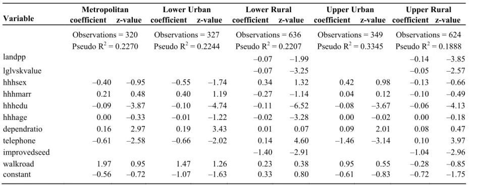
Table 5 provides estimated results from the reduced form Probit model for poverty status. Again, education, dependent ratio, and telephone availability are revealed as determinants of household poverty status.
As previously mentioned, community characteristics could be well exploited when rural sectors only were considered. Similar to the case of strata, the educational attainment of the household head and the dependent ratio are universally related to total income, expenditure, and poverty status in both lower and upper rural Egypt (Table 6). In general, the community characteristics do not provide significant welfare effects on expenditure or poverty, except for the existence of preschool, paved roads in lower rural areas. In lower rural Egypt, infrastructure—such as a post office, bus stop, and access to an agricultural extension worker—help residents to increase their total incomes, while (public and commercial) canal service decreases incomes. Some of the community-level variables may have a high correlation with household access to public services such as distance to paved roads, access to a telephone, and the use of modern seeds.
The household-level analysis provides information on how household and community characteristics correlate with household income and poverty status. But there are several disadvantages. It is difficult, for example, to control for endogeniety and multicollinearity problems unless there is a long time series of household panel data. In addition, household-level analysis cannot capture the market-, regional-, and macro-level effects resulting from various government interventions. Finally, it is difficult to link improved public provisions to meaningful government investment programs. Therefore, regional- and macro-level analyses are required to complement the household-level analysis.
Table 5. Estimated Results of the Poverty Equation, the Reduced Form
Metropolitan Lower Urban Lower Rural Upper Urban Upper Rural
Variable coefficient z-value coefficient z-value coefficient z-value coefficient z-value coefficient z-value
Observations = 320 Observations = 327 Observations = 636 Observations = 349 Observations = 624 Pseudo R2 = 0.2270 Pseudo R2 = 0.2244 Pseudo R2 = 0.2207 Pseudo R2 = 0.3345 Pseudo R2 = 0.1888
landpp –0.07 –1.99 –0.14 –3.85 lglvskvalue –0.07 –3.25 –0.05 –2.57 hhhsex –0.40 –0.95 –0.55 –1.74 0.34 1.32 0.42 0.98 –0.13 –0.66 hhhmarr 0.21 0.48 0.40 1.19 –0.27 –1.14 0.04 0.12 –0.10 –0.49 hhhedu –0.09 –3.87 –0.10 –4.74 –0.11 –6.52 –0.08 –3.67 –0.06 –4.13 hhhage 0.00 –0.33 –0.01 –1.22 –0.02 –3.28 0.00 –0.02 0.00 –0.18 dependratio 0.16 2.97 0.19 3.43 0.01 0.07 0.09 2.01 0.08 0.47 telephone –0.61 –2.58 –0.66 –2.02 0.14 4.60 –1.46 –3.14 0.10 3.97 improvedseed –1.40 –2.91 –1.04 –2.96 walkroad 1.97 0.95 1.47 1.26 0.23 0.38 0.95 0.55 –0.28 –0.85 constant –0.56 –0.72 –1.07 –1.63 0.33 0.80 –0.61 –0.83 –0.72 –1.75
Table 6. Estimates of Total Income Per Capita, Total Expenditure Per Capita, and Poverty Status with Community Variables
Note: Pavedroad and prepschool are dropped due to collinearity.
lgtotipp lgexppp poor
Lower Rural Upper Rural Lower Rural Upper Rural Lower Rural Upper Rural
Variable coefficient t-value coefficient t-value coefficient t-value coefficient t-value coefficient t-value coefficient t-value
Observations = 416 Observations = 503 Observations = 406 Observations = 499 Observations = 406 Observations = 499
R2 = 0.3868 R2 = 0.3147 R2 = 0.2961 R2 =0.3111 Pseudo R2 = 0.2748 Pseudo R2 = 0.2229 landpp 0.03 3.07 0.02 1.77 0.01 1.08 0.01 1.56 –0.13 –1.78 –0.14 –3.67 lglvskvalue 0.05 3.64 0.05 4.50 0.01 1.39 0.03 3.03 –0.08 –2.36 –0.07 –3.01 hhhsex –0.04 –0.24 –0.22 –1.76 –0.18 –1.61 0.06 0.75 0.16 0.46 –0.09 –0.39 hhhmarr 0.02 0.12 –0.20 –1.50 0.13 1.19 –0.09 –1.07 –0.17 –0.53 0.04 0.15 hhhedu 0.04 5.65 0.04 4.46 0.03 6.63 0.03 5.65 –0.09 –4.00 –0.07 –3.68 hhhage 0.01 2.43 0.01 2.06 0.01 3.22 0.00 1.48 –0.02 –2.35 0.00 –0.50 dependratio –0.13 –6.86 –0.08 –5.57 –0.06 –4.33 –0.05 –4.84 0.13 3.09 0.11 3.57 telephone 0.05 0.45 0.27 1.93 0.22 3.07 0.37 3.78 –1.21 –2.85 –1.06 –2.76 improvedseed 0.40 4.47 0.49 5.84 0.09 1.64 –0.01 –0.19 –0.28 –1.11 0.17 0.90 walkroad –0.73 –1.81 0.11 0.61 0.09 0.46 –0.09 –0.60 –0.91 –0.90 –0.28 –0.74 postoffice 0.37 2.47 –0.06 –0.29 0.01 0.12 0.09 0.59 0.02 0.06 –0.01 –0.02 commbank –0.19 –0.67 –0.27 –1.19 0.23 1.26 0.19 1.04 –0.20 –0.27 –0.74 –1.44 market 0.26 1.35 –0.48 –1.99 0.14 1.07 –0.04 –0.33 –0.56 –1.04 –0.93 –1.96 prepschool –0.83 –3.51 –0.38 –2.96 1.62 2.93 busstop 0.39 2.48 0.16 0.93 0.09 0.97 0.13 1.11 –0.63 –1.84 –0.13 –0.39 pavedroad –0.28 –1.64 –0.19 –2.07 0.36 1.22 agextn 0.30 1.72 –0.13 –0.71 0.15 1.28 –0.06 –0.48 –0.40 –0.87 0.26 0.77 clinic 0.27 1.50 0.00 –0.03 –0.13 –1.16 –0.02 –0.20 0.10 0.23 –0.18 –0.72 pubcanal –0.68 –2.46 0.23 1.04 0.05 0.35 0.09 0.59 –0.03 –0.04 –0.14 –0.33 commcanal –0.56 –2.62 0.06 0.42 –0.24 –1.81 –0.10 –1.22 0.68 1.14 0.29 1.18 constant 6.90 21.56 6.30 13.66 7.39 20.88 6.80 22.21 0.21 0.23 –1.39 –1.56
V. REGIONAL LEVEL ANALYSIS
This section of the report evaluates the impact of various government investments on agricultural growth and poverty reduction using data from different governorates for the period 1980–2000. This level of analysis captures some of the effects that the household- level analysis cannot capture, such as effects on labor and product markets. The Model
Public investment affects rural poverty through many channels. It directly increases farmer incomes by increasing agricultural productivity, which in turn reduces rural poverty. Indirect impacts include higher agricultural wages and improved nonfarm employment opportunities. In addition to its productivity impact, public investment directly promotes rural wages, nonfarm employment, and migration, thereby reducing rural poverty.
Public investments in rural sectors not only contribute to growth, employment, and wages in rural areas, but also help the development of the national economy by providing labor, human and physical capital, cheaper food, and markets for urban industrial and service development. Growth in the national economy reduces poverty in both rural and urban sectors. In an era of macroeconomic reforms, understanding these different effects provides useful policy insights to improve targeting efficiencies, budgeting, and ultimately the effectiveness of government poverty reduction strategies.
Few studies have linked poverty reduction to the driving forces behind economic growth and income distribution. The determination of rural poverty adds a greater complexity. Rural residents draw their income from multiple sources. Farm activities are still major sources of income for many rural residents, but nonfarm activities such as rural industry and services have increasingly become important. Another important income source is seasonal migration and employment in the urban sector. Building on earlier work on India (Fan, Hazell, and Thorat 1999), rural poverty determination is modeled as follows:
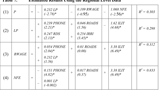
Equation (9) models the determinants of rural poverty (P), which is defined as the percentage of the rural population living below the poverty line. They include agricultural labor productivity (LP), nonagricultural employment (NFE), and rural wages (RWAGE).
Equation (10) models the agricultural labor productivity function. The dependent variable is the gross value of agricultural production per agricultural worker in the agricultural sector (LP). The independent variables are a set of technology, infrastructure, and education variables used to capture their impact on labor productivity growth. These variables include agricultural research stock variables constructed from past government expenditures on agricultural research and development (RDS), irrigated areas (IRRIA) per agricultural worker, the illiteracy rate of the rural population (ILIT), the length of rural roads per agricultural worker (ROADS), and the number of rural telephones per agricultural worker (PHONE).
LP =
ƒ
(RDS, IRRIA, ILIT, ROADS, PHONE). (10) Equations (11) and (12) are wage and nonfarm employment determination functions. Rural nonfarm wages and employment are determined by developments in infrastructure, improved education, and growth in agricultural productivity. Growth in agricultural productivity is included to model the linkage between growth in the agricultural sector and nonfarm employment and rural wages.RWAGE =
ƒ
(LP, ROADS, PHONE, ILIT). (11)NFE =
ƒ
(LP, ROADS, PHONE, ILIT). (12)The marginal impact of public capital expenditures on poverty can be derived from this system of equations by taking the total derivatives, as follows, using agricultural research and rural education as examples:
dP/dRDS = (∂P/∂LP)(∂LP/∂RDS)
+(∂P/∂NFE)(∂NFE/∂LP)(∂LP/∂RDS)
dP/dILIT = (∂P/∂LP)(∂LP/∂ILIT)
+(∂P/∂NFE)(∂NFE/∂LP)(∂LP/∂ILIT)
+(∂P/∂RWAGE)(∂RWAGE/∂LP)(∂LP/∂ILIT) +(∂P/∂NFE)(∂NFE/∂ILIT)
+(∂P/∂RWAGE)(∂RWAGE/∂ILIT). (14) Equation (13) measures the marginal effect on poverty reduction of the research stock variable. It also decomposes the different pathways through which impacts occur (see Fan, Hazell, and Thorat 1999 for a more detailed discussion). The first term on the right-hand side is the direct poverty impact of growth in agriculture due to agricultural research and extension, while the remaining terms measure the effects of agricultural research and extension through improved nonfarm employment and wages.
Equation (14) is the marginal poverty reduction effect of improved education. Similar to equation (13), the first three terms on the right-hand side are poverty reduction effects of improved education both directly and indirectly through growth in agricultural production by improving nonfarm employment opportunities and rural nonfarm wages. The last two terms capture the poverty reduction impact by directly improving nonfarm employment and nonfarm wages.
To convert annual government expenditures on public capital into stocks in monetary terms, we use the following procedure:
. K δ) (1− t-1 + = t t I K (15)
where Ktis the capital stock in year t, Itis gross capital formation in year t, and δ is the
depreciation rate (5 percent). To obtain initial values for the capital stock, we used a similar procedure to Kohli (1982):
. ) r (δ 0 0 = + I K (16)
Equation (16) implies that the initial capital stock in year 0 (K0) is capital
investment in year 0 (I0) divided by the sum of the real interest rate (r) and the
Sensitivity analyses were conducted to determine whether different depreciation rates and real interest rates would affect our final results. We found the impact of different real interest rates to be negligible. But different depreciate rates do result in some differences.7Nevertheless, the ranking of returns among different types of investment and
across regions remains the same.
Obtaining stocks for various types of public investment enables the following regressions to be run to determine the relationship between these stocks, in monetary terms, and physical stocks:
P i,t=f(K i,t, Z i,t), (17)
where Pi,t is physical stock of public investment, i, in year t—for example, road density,
years of schooling, rural literacy rate, electricity consumption, or irrigated areas—and Ki,t
is capital stocks in monetary terms for investment i in year t constructed from equation (15). To control other factors that may be omitted from the equation (Z i,t ), both year and
regional dummies are added during the estimation.
To calculate the marginal return, in terms of poverty reduction, of different types of government spending such as roads, education, and irrigation, we use derivatives of the following form, using education as an example:
dPt /dKe,t = dPt /dILITt* ∂ILITt /∂Ke,t . (18)
Equation (18) implies that the marginal return to capital stock in education (Ke,t)
is the product of the marginal return to improved literacy (derived in Equation (14)) and marginal impact of capital stock on the years of schooling.
7 Sensitivity analyses of different interest and depreciation rates for roads were conducted for the following scenarios: (a) 3 percent real interest rate and 10 percent depreciation rate, (b) 5 percent real interest rate and 10 percent depreciate rate, (c) 3 percent real interest rate and 5 percent depreciation rate, and (d) 5 percent real interest rate and 5 percent depreciation rate. The estimated marginal returns were 0.86, 0.84, 0.61, and 0.63, respectively.
Data
Most of the data used in this study come from various agencies of the Egyptian government.
Poverty. The poverty variable is measured as the percentage of the rural population living below the poverty line.
Agricultural labor productivity. Agricultural labor productivity is measured as gross agricultural production value per agricultural worker.
Nonfarm employment. Rural nonfarm employment is measured as the percentage of the rural labor force engaged in nonfarm activities such as manufacturing, construction, trading, and services.
Wages. Rural wages are the average daily compensation for rural workers.
Agricultural research. Agricultural research in Egypt is conducted at the national level, but national research affects production throughout the country through spillover effects. Therefore, we include the same agricultural research stock variable constructed from past expenditures in all regions. When we calculate returns to agricultural research investment, we also add agricultural extension to determine total investment in agricultural R&D.
Infrastructure. Most of the infrastructure and education variables used in the model are defined in physical terms and data for suitable measures are available at the national and regional levels. The greatest difficulties arose in collecting data on government expenditure by type of investment and region, which are needed for calculating the value of the existing stocks of these investments and their unit costs. Like many countries, Egypt compiles data on public spending by different types of investments at the national level, but there is much less data on how these expenditures are allocated to different regions. Therefore, some techniques and assumptions had to be used to make these allocations.
Irrigation. Both irrigated areas and investment costs are available at the regional level.
Rural education. The illiteracy rate is used to proxy the improvement in education.
Roads. Road length and public expenditure data on roads are available by region from the government office.
Rural telephones. The number of telephones (that is, handsets) is used as a proxy for improved telecommunications.
Model Estimation
We use the double-log functional forms for all equations in the system. More flexible functional forms, such as translog or quadratic equations, impose fewer restrictions on the estimated parameters, but many coefficients are not statistically significant due to multicollinearity problems. Regional dummies are added to equations of poverty, productivity, employment, migration, and terms of trade to capture the fixed effects of regional differences in agroclimatic and socioeconomic factors. The time trend variable is also added to these equations, with the exception of the poverty equation, to control for any macroeconomic polices that have the same impact on every region. The model is estimated for the period 1981–2000.
There are two approaches in estimating an equation system: the single equation approach and the multiple equation (systems) approach. Single equation techniques, such as instrumental variable estimators, two-stage least squares, and limited information maximum likelihood are easy to estimate and require only limited information. However, the single equation technique often neglects information contained in the other equations of the system. For this reason, we use the full information maximum likelihood (FIML) estimation technique. Among all estimators, FIML is the most efficient. The only disadvantage is its estimation complexity but with the rapid development of econometric software, this task has become increasingly easier and more accessible.8
Rural poverty is negatively correlated with labor productivity, rural wages, and the level of nonfarm employment (Equation 1), but rural wages is not statistically significant (Table 7). The insignificance of rural wages on nonfarm employment is similar to the findings in many Asian countries (Thailand and Vietnam). This may indicate that there is an inelastic supply of rural labor or a large labor surplus in these economies. Rural nonfarm employment has the largest poverty reduction elasticity among all explanatory variables. The estimated agricultural labor productivity equation indicates that improvements in access to telephones and rural education has a large impact on labor productivity. In particular, a higher illiteracy rate is strongly correlated with lower labor productivity, with an elasticity of –1.16. The roads variable is also correlated with labor productivity but is not statistically significant. Equations (3) and (4) show that development in telecommunications (proxied by telephones) and improvements in education are statistically significant in promoting rural wages and nonfarm employment. Rural roads, however, are not statistically significant. Improved labor productivity is also not statistically significant in helping to increase rural wages and nonfarm employment.
Table 7. Estimated Results Using the Regional Level Data
(1) P = – 0.232 LP (–2.78)* – 0.109 RWAGE (–0.95) – 1.068 NFE (–2.56)* R2 = 0.303 (2) LP = + + 0.239 PHONE (2.21)* 0.247 RDS (2.13)* + + 0.046 ROADS (1.56) 0.254 IRRI (3.45)* – 1.62 ILIT (4.68)* R2 = 0.298 (3) RWAGE = + + 0.054 PHONE (2.04)* 0.232 LP (1.56) + 0.01 ROADS (0.00) + 3.38 ILIT (6.49)* R 2 = 0.312 (4) NFE = – – 0.151 PHONE (4.82)* 0.001 LP (–0.002) + 0.017 ROADS (0.37) + 3.38 ILIT (6.49)* R2 = 0.833
Marginal Returns in Agricultural Growth
We first calculate the marginal returns in agricultural growth per additional physical unit. Then, using the parameters estimated through equations (9) through (12), we are able to calculate the unit cost of public capitals. Comparing the unit cost with the marginal benefit, we can easily estimate benefit–cost ratios (Table 8).
Table 8. Effects of Public Investment on Agricultural Growth
Region Phone Roads Education R&D Irrigation Benefit–cost ratio
Metropolitan 0.25 0.31 n.a. 7.89
Lower Egypt 6.37 3.73 5.81 1.85
Upper Egypt 4.36 4.79 4.43 1.97
Egypt 3.13 2.84 4.86 4.12 1.94
Poverty reduction effect, number of poor per 1 million LE
Metropolitan 17.31 21.19 9.98 545.16
Lower Egypt 129.68 75.97 59.15 37.56
Upper Egypt 335.27 368.40 170.53 151.42
Egypt 133.95 121.47 208.26 176.31 83.16
For telephones, the national average benefit–cost ratio is 3.13. However, in metropolitan area, the ratio is less than one, meaning that the return from investments in telephones does not cover the cost. For lower Egypt, the ratio is more than 6, which indicates that the returns from agricultural production are six times greater than its cost. If we include the effect on nonfarm GDP and rural GDP, the benefit–cost ratio would be much larger. Upper Egypt has a ratio of 4.36. The national average benefit–cost ratio of road investment is 2.84. Again, the benefit–cost ratio in the metropolitan area is less than one. The largest return is in upper Egypt, where the ratio is 4.8. Lower Egypt has a ratio of 3.7. Education investment has the highest return among all types of investment with a benefit–cost ratio of 4.8 nationally. Lower Egypt has the highest marginal return with a benefit–cost ratio of 5.8. Upper Egypt has a ratio of 4.4—75 percent of the effect in lower Egypt. Irrigation has the lowest benefit–cost ratio among all types of investments with a ratio of 1.94. It suggests that irrigation is still a good investment (note that this
ratio is high compared with Asia).9 Among all investment, at the national level, education
ranks first, followed by agricultural R&D, telephones, roads, and irrigation. For lower Egypt, telephones and roads have high returns, followed by education and irrigation. For upper Egypt, roads rank first, followed by telephones and education, which have similar marginal returns. Similar to other regions, irrigation has the lowest returns.
Marginal Returns in Poverty Reduction
Similar to returns in agricultural growth, we calculate returns in poverty reduction in terms of both physical and monetary units (Table 8 presents the estimated number of poor reduced per thousand LE). At the national level, education has the largest impact per unit of investment. For every million LE investment, more than 200 poor people would be lifted above the poverty line. Agricultural research closely follows the education effect. The poverty reduction effect is 176 for every million LE invested. Two infrastructure variables, telephones and roads have similar poverty reduction effects per unit of spending. Irrigation investment has the smallest marginal impact on poverty reduction, and its effect is only 40 percent of the education effect and 47 percent of the R&D effect.
Large regional differences occur in the marginal effect of different investments. With the exception of irrigation, all kinds of investment have the largest impact in upper Egypt. Except for irrigation, all kinds of investment in Metropolitan area have the lowest marginal impact.
9 In the case of India, the benefit–cost ratio of irrigation is less than one (Fan, Hazell, and Thorat 1999). For China, the ratio is marginally above one (Fan, Zhang, and Zhang 2002).