Civil Engineering Journal
Vol. 5, No. 8, August, 2019Improving Equipment Reliability and System Maintenance and
Repair Efficiency
A.Yu. Rusin
a*, Ya.V. Baryshev
aa Tver State Technical University, Department of Power Supply and Electrical Engineering, Naberezhnaya Afanasiya Nikitina, 22, Tver,
Tver region, 170026, Russia. Received 12 March 2019; Accepted 29 June 2019
Abstract
Mean time to failure of modern machinery and equipment, their individual parts and components can be calculated over the years. Methods for determining the optimal frequency of maintenance and repair, based on the collection and processing of information about the reliability of industrial facilities, during their testing in laboratories and at special sites, as well as through long, operational tests require considerable time and become expensive. The purpose of this work is to develop methods for processing information about the reliability of equipment in automated systems for maintenance and repair, which will reduce the time to collect information on equipment failures and improve the cost-effectiveness of maintenance and repair. Small, multiple-censored right-side samples of equipment operating time for failure are formed as a result of failure data collection in an automated system for equipment maintenance and repair. Calculation of reliability indicators for such samples is performed using the maximum likelihood estimation method. The article presents experimental studies of the accuracy of the maximum likelihood estimates of the parameter of the exponential distribution law for small, multiple right-censored samples. The studies were carried out by computer modeling of censored samples, similar to samples that are formed when monitoring equipment during operation. Methods of simulation modeling of random processes on a computer and methods of regression analysis were used. Analysis show that most of the maximum likelihood estimates obtained from small, multiple-censored right-side samples have significant deviations from the true values. A technique for improving the accuracy of maximum likelihood estimates is proposed. The scientific novelty is regression models are constructed that establish the relationship between the deviation of the maximum likelihood estimate from the true value and the parameters characterizing the sample structure. These models calculate and introduce corrections to maximum likelihood estimates. The use of the developed regression models will reduce the time to collect information about the reliability of the equipment, while maintaining the reliability of the results.
Keywords: System Maintenance and Repair; Equipment Reliability; Censored Samples; Maximum Likelihood Method; Computer Simulation.
1.
Introduction
The essence of the system maintenance and repair lies in the fact that after a certain amount of time worked, various types of repair work are carried out aimed at restoring the equipment (maintenance, current or capital repairs). The system of maintenance and repair is a regulatory information base necessary for the development and scheduling of maintenance and repair. It contains the scope of work for maintenance, current or capital repairs; structure and frequency of maintenance and repair; norms of labor intensity and repair time; consumption rates of basic materials, components, spare parts; reserve standards. Regulatory and information base is formed on the basis of industry average indicators. As
* Corresponding author: [email protected] http://dx.doi.org/10.28991/cej-2019-03091372
© 2019 by the authors. Licensee C.E.J, Tehran, Iran. This article is an open access article distributed under the terms and conditions of the Creative Commons Attribution (CC-BY) license (http://creativecommons.org/licenses/by/4.0/).
a result, uniform standards and rules for maintenance and repair are applied at enterprises that differ: in the climatic conditions in which the industrial equipment operates, its service life and its degree of wear, type and performance, and qualifications of the service personnel. Therefore, these rules may not be optimal for this particular enterprise.
The lack of a connection between the operating conditions of the equipment in the enterprise and the regulatory base of the system leads to the fact that the current the system maintenance and repair hampers the development and introduction of new technologies in repair. Improving repairs, introducing technical diagnostics methods to periodically monitor the condition of the equipment increases the operational reliability of the equipment. However, the frequency of planned work, which is determined by current regulations, does not change. As a result, the costs associated with the introduction of new developments do not pay off.
In some studies such as Chin-Chih (2014), Kizim (2016), Baskakova et al. (2016) and Knopik and Klaudiusz (2019), the authors concluded that the principles of strict regulation of the structure and duration of the repair cycle have a negative impact on the efficiency of the maintenance and repair system [1-4]. It is noted that the duration of the repair cycle must be different even within the framework of one model of tools, machines, since the service life of the elements of various tools, machines is different. Also, the stochastic process of wear and difference between the lifetimes of tools and machines represents additional conditions that are not taken into account by the system. Planning and calculation of indicators and standards based on repair units cannot take into account the individual characteristics of the machines, operating conditions and varying degrees of depreciation, the degree of technical preparation for production, and the technological level. The existing branch of maintenance and repair is built on this basis. Repair units are a specific type of equipment. To develop standards for the system maintenance and repair of individual elements of electrical equipment, it is necessary to perform an analysis of electrical equipment failures when collecting information about reliability. On the scale of the entire industry, it is practically impossible to carry out this work due to the high material costs and the difficulty of obtaining reliable information.
Liu et al. (2019), it was recommended to adjust the system maintenance and repair, developed in the design of machines, during operation. Adjustment is necessary because of the random nature of the operation of machines and the random change in their technical condition, accumulated experience in the operation of machines[5].With each frequency adjustment, the system maintenance and repair perform the following major tasks:
Assessment of reliability indicators and development of a list of changes to the current the system maintenance and repair;
Development of recommendations for improving the methods of the system maintenance and repair;
Verification of the results of the adjustment of the system maintenance and repair on a limited number of machine samples by conducting their trial operation;
Final development of the maintenance system for all machines in operation and its implementation.
Most of all, this principle is implemented in the USA, where, as noted by Jianming et al. (2019), Ditho et al. (2018), Shojaei and Volgers (2017) and Yan-qing et al. (2014), there is a complete lack of a standard approach in choosing strategies and tactics, forms of maintenance and repair in each specific case, since it is considered that each enterprise is unique in its own way and there are no two similar [6-9].
These deficiencies can be eliminated by creating and implementing the system maintenance and repair at enterprises, which links the frequency of the system maintenance and repair with the operational reliability and technical condition of electrical equipment.
Adaptability of the system maintenance and repair is the property that can be described as the ability of the system to self-adjust, adapt to changes in the factors characterizing the operation process, equipment operating conditions, and changes in the reliability of electrical equipment. The adaptability of the system maintenance and repair is provided by changing the schedule of maintenance and repair in accordance with changes in the reliability of the equipment of the enterprise or its structural unit (shop, site). This is achieved by the fact that the period between the various planned work of the system maintenance and repair is calculated on the basis of mathematical models of maintenance, repair and overhaul, taking into account the distribution of time between failures, average recovery time and other indicators of the reliability of electrical equipment. The system maintenance and repair schedule is constantly updated as information on equipment reliability is accumulated and updated.
According to the modern level of development of science and technology, an automated system for maintenance and repair should perform the following functions:
Accumulation of statistical information on equipment failures and its individual structural elements. Finding the law of distribution of time between failures of equipment and the calculation of its parameters;
Calculation of the optimal frequency of maintenance and repair for this type of equipment and its individual structural elements;
Analysis of equipment failures, allowing for the calculation of the frequency of maintenance, current and capital repairs to take into account only those failures, the causes of which are eliminated as a result of the corresponding type of maintenance and repair;
The creation and maintenance of a regulatory information base for maintenance and repair for various types of electrical equipment and some of the most frequently denying its elements.
Thus, an automated maintenance and repair system should be an integrated environment designed to accumulate information about equipment failures and its technical condition, optimize the maintenance and repair system, and systematize the experience of maintenance personnel.
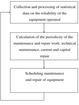
The general algorithm of functioning of the adaptive system of maintenance and repair is shown in Fig.1. To determine the mean time between failures and average recovery time, the collection and processing of statistical information about equipment reliability is organized. Then, using mathematical models of maintenance and repair, using the found reliability indicators and the distribution function of add-ons for failure, the frequency of maintenance and repair works is calculated. At the last stage, a maintenance and repair schedule is drawn up. After a certain period of time, after updating the statistical information about the reliability of electrical equipment, the calculation cycle is repeated and a new maintenance and repair schedule is compiled, corresponding to a new level of reliability.
From the algorithm of functioning of the adaptive maintenance and repair system (Figure 1), it can be seen that the main elements of the mathematical support of the system are the methods of processing statistical information about equipment reliability and mathematical models of maintenance and repair, designed to calculate the recovery interval.
Collection and processing of statistical data on the reliability of the
equipment operated
Calculation of the periodicity of the maintenance and repair work: technical
maintenance, current and capital repair
Scheduling maintenance and repair of equipment
Figure 1. Algorithm of functioning of the automated system of maintenance and repair
The Bykhelt and Franken (1988) describes the main strategies for work in the system of maintenance and repair, equipment recovery strategies, and proposed Equation 1-6 for calculating the recovery interval [10].
Strategy 1. If the object has worked without failures for a specified time interval, then preventive maintenance is carried out. Restorations that are made after failures are called abnormal. Both preventive and disaster recovery are complete. The intensity of operating costs 𝑅() is calculated by the Equation 1:
R C F C F F t dt ( ) ( ) ( ) ( )
a n 0 (1) Where С𝑎: Average disaster recovery costs; 𝐶п: Average preventative recovery costs; : Maintenance period; 𝐹(𝑡): functions of distribution of time between failures.This опт. is a solution to the equation 𝑑𝑅()/𝑑= 0 or:
( )F t dt F( ) ( ) C C
1 0 (2)Where (𝑡): failure rate function
.
Strategy 2. In case of failure, the object undergoes disaster recovery, which is the minimum recovery. Regardless of the age of the system, preventive maintenance is systematically carried out at fixed points in time, that is, full recovery is carried out.
Intensity of operating costs: R t( )CпСа ( )
(3)
Where Λ (𝑡) cumulative failure rate:
( )
( )t dtt
0
(4) The optimal recovery interval опт is a solution to the Equation 5:
( )( ) C C
п а
(5)
The most common solution to the problem of optimizing maintenance, repair and selection of the optimal recovery interval is given by Barzilovich (1982) [11]. The optimal service period is determined by the criterion of the maximum operational readiness ratio from the Equation 6:
T T T x F t dt F T T T x п a п п a п
( ) ( ) ( ) ( ) 0 (6)Where 𝑇п: time (or cost) of prevention; 𝑇𝑎: time (cost) of emergency repair. Similar models using the distribution function F(t) are given in many other works.
It can be seen from Equation 1-6 that the economic efficiency of the automated maintenance and repair system is largely determined by the accuracy of estimates of the equipment failure distribution law, since the main element of the models for calculating the optimal maintenance and repair period is the distribution of time between failures. Improving the accuracy of maximum likelihood estimates is directly related to the increase in the economic efficiency of an automated maintenance and repair system.
In almost all problems of reliability, the main requirement for methods of processing statistical information is to ensure the required accuracy, efficiency and reliability of estimates of the distribution function parameters and reliability indicators.
When calculating the reliability indicators and parameters of the law of distribution of equipment failures of a single enterprise and its structural subdivision (shop, site), the number of installed equipment of the same type is in most cases insufficient to form complete samples of time to failure for available observation times. Therefore, the creation of an automated maintenance and repair system with the functions of calculating the period of maintenance and repair, corresponding to the operating conditions and reliability of the electrical equipment of an individual enterprise, sets the task of estimating the parameters of the failure distribution function for small, repeatedly censored samples.
2.
Materials and Methods
The main method of calculating reliability indicators for censored samples is the maximum likelihood method. The essence of the maximum likelihood method is as follows [12, 13]. The likelihood function is constructed for sampling random variables with a known distribution law. The likelihood function is:
L
A
f t
iF
j j m i n
( )
1
( )
1 1
(7)Where А: Constant rate; 𝑡𝑖: Time to failure of the observed object; 𝑗: Censored operating time; 𝑛: Number of failures;
𝑚: Number of censored operating time; 𝐹(𝑡): Functions of distribution of time between failures; 𝑓(𝑡): Distribution density.
To find the maximum likelihood estimates of the exponential distribution, it is necessary to solve the Equation 8: 0 ln t L (8)
For the exponential law, the distribution density and the distribution function are respectively equal to: f t( )et
(9)
F t( ) 1 et (10)
The likelihood function is
L
f t
( )
1
f t
( )
2
f t
( )
r
F
( )
1
F
( )
2
F
( )
n (11) After substitution (9) and (10) in (11), take the logarithm likelihood functionlnL r ln ti j i r j n
1 1 (12)Where : exponential distribution parameter; 𝑡: operating time to failure; : operating time to censoring; 𝑟: the number of operating time to failure; 𝑛: the number of operating time to censoring.
Differentiating Equation 12 by and equating to 0, we get:
lnL r ti j j n i r
1 1 0 (13)From Equation 13, we obtain the point estimate of the parameter of the exponential distribution:
r ti j j n i r 1 1 (14)The article presents experimental studies of the accuracy of the maximum likelihood estimate for the parameter of the exponential distribution law for small, multiple right-censored samples. Such samples arise during the observation of failures during operation or when testing according to the plan [N, U, Z].
[N, U, Z] – is a test plan, according to which N objects are tested simultaneously. The objects that failed during the tests do not restore or replace, each object is tested during the operating rime zi i, where 𝑧𝑖= 𝑚𝑖𝑛(𝑡𝑖, 𝜏𝑖), ti – is the operating time to failure, τi is the operating time before i–th object is removed from the test.
The studies were carried out using computer modeling of censored samples, similar to samples formed in the course of studying equipment reliability indicators in an automated system for maintenance and repair.
To conduct research, an algorithm and a program for simulating the process of computer failures arising during tests according to the plan [N, U, Z] have been developed.
The following algorithm was used to form the sample that was censored to the right several times:
1. A random variable t is generated, distributed according to the studied exponential distribution law, calculated by the Equation 15; R z 1ln (15)
Where 𝑅: random variable uniformly distributed over the interval (0, 1).
2. A random variable is generated, distributed according to a censoring distribution law. The right-truncated normal distribution law was used as a censoring law.
3. The resulting random variables are compared. If (𝑡 <), a random variable t is added to the simulated sample, which corresponds to the time to failure. If (𝑡 >), a random variable is added to the simulated sample, which corresponds to the operating time before censoring.
4. The modeling process continues until the number of random variables obtained becomes equal to a given number of members of the sample N (sample size).
The computer simulated samples of random variables that were repeatedly censored on the right, of volume 𝑁 =
5, 10, 15, 20, 25. The generation of samples was carried out under the following restrictions
5 𝑁 < 10, 𝑞 0.5 10 𝑁 < 20, 𝑞 0.3 20 𝑁 50, 𝑞 0.2
Where q – degree of sample censoring.
The number of formed samples V for each value of N is 3000. For each sample, the maximum likelihood method was used to calculate the estimates of the exponential distribution and their relative deviations from the true values using the Equation 17:
ОМП (17)Where 𝜆: true value of the exponential distribution parameter; 𝜆𝑂𝑀𝜋: maximum likelihood estimate of the exponential distribution.
The studies posed the problem of studying the accuracy of maximum likelihood estimates for various samples. Therefore, the parameter 𝜆 of the studied distribution law was calculated for each generated sample using a random number uniformly distributed over the interval [0, 1] according to the Equation 18:
𝜆 = 0.6 + 0.4 × 𝑅𝐴𝑁𝐷() (18) Where 𝑅𝐴𝑁𝐷() is the function of generating a random number uniformly distributed on the interval [0, 1].
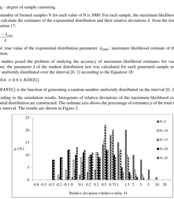
According to the simulation results, histograms of relative deviations of the maximum likelihood estimates of the exponential distribution are constructed. The ordinate axis shows the percentage of estimates p of the total number falling into this interval. The results are shown in Figure 2.
Figure 2. Relative deviations of the maximum likelihood estimate
These experimental data show that most of the maximum likelihood estimates obtained from small, repeatedly censored samples from the right, have significant deviations from the true values. For example, 1% of the estimates of the exponential distribution for N = 5 have relative deviations from 10 to 20; 4% - from 5 to 10; 8% - from 3 to 5. With increasing sample size N, the accuracy of the estimates increases. When N = 25, the relative deviations of the estimates of the exponential distribution law do not exceed 2. Despite this, 2% of the estimates have relative deviations from 1.5 to 2; 3% - from 1 to 1.5; 9% - from 0.75 to 1; 12% - from 0.5 to 0.75. At N = 5, 10, 15, a strong shift in the maximum likelihood estimates is clearly visible.
In general, we can conclude that the accuracy of the maximum likelihood method for values of 𝑁 < 25 is low. The relative deviation of estimates from the true values can reach 3 or more, and half of all estimates have deviations greater than 0.3, depending on the sample size.
This article proposes a method for improving the accuracy of maximum likelihood estimates for small, repeatedly censored samples during tests carried out according to the [N, U, Z] plan.
The purpose of the conducted research in general form can be formulated as follows: obtaining mathematical models that establish a relationship between the relative deviation of the maximum likelihood estimates from the true value of the exponential distribution parameter and parameters characterizing the sample structure.
The solution of the task consisted of the following stages:
1. Computer simulation of samples of random variables repeatedly censored to the right, distributed according to the exponential law, according to the algorithm described above.
0 5 10 15 20 25 -0.8 -0.5 -0.3 -0.2 -0.1 0 0.1 0.2 0.3 0.5 0.75 1 1.5 2 3 5 10 20 p (%) N=5 N=10 N=15 N=20 N=25
To avoid repetition of pseudo-random number sequences, a random number was generated based on system time before each sample was formed. To do this, we used the standard 𝑅𝐴𝑁𝐷(−1) function with a negative argument -
𝑅𝐴𝑁𝐷(−1). Obtaining a sufficient difference in the system time, when generating samples, was carried out using a time delay of up to 30 milliseconds before each cycle of forming a repeatedly censored sample.
2. Calculation of sample parameters characterizing its structure. To describe the structure of the formed sample of random variables, we used five standard sampling parameters [14, 15]:
Degree of censoring
N k q
X1 (19)
Where 𝑘: number of complete random variables, 𝑁: the number of members in the sample.
The coefficient of variation:
Z S
X2 (20)
Where 𝑆: estimation of the standard deviation of all random variables in the sample; 𝑍̅: expected value of all members of the sample.
Coefficient of variation of total random variables:
Z S
X3 П (21)
Where 𝑆𝜋: estimation of the standard deviation of total random variables.
Empirical skewness coefficient:
3 2 3 4 ~ Z z Z z A X (22) Coefficient of kurtosis: 3 ~ ~ 4 4 5 S E X (23)Where 𝜇̃:4 central moment of the fourth order.
Another five parameters are mathematical expressions made up of standard sampling characteristics;
The ratio of the expectation of total random variables to the expectation of all members of the sample:
Z Z
X6 П (24)
The ratio of the expectation of censored random variables to the expectation of all members of the sample:
Z Z
X7 Ц (25)
Relative deviation of the expectation from the middle of the variation range:
Z Z R X 2 8 (26)
Where 𝑅 = 𝑍𝑚𝑎𝑥 – 𝑍𝑚𝑖𝑛; variation scale, 𝑍𝑚𝑎𝑥, 𝑍𝑚𝑖𝑛: respectively, the maximum and minimum value of a random variable.
Relation of median to expectation of random variables:
Z M X e ~ 9 (27) Where 𝑀̃𝑒 median.
Z M
X10 o
~
(28)
All parameters are measured in relative units and do not depend on the absolute values of random variables. This has achieved the adequacy of the regression equations obtained in an experiment on a computer with regression equations describing similar dependencies for a set of samples of failures that are formed during the observation of the equipment.
3. Calculation of maximum likelihood estimates of the parameter of the exponential distribution law.
4. Calculation of the dependent parameter - the deviation of the maximum likelihood estimate from the true value by the Equation 29: ОМП y (29)
5. Building regression dependencies. As a result of the research, regression mathematical models were constructed that establish a connection between the deviation of the maximum likelihood estimate from the true value and the parameters characterizing the sample structure. For each sample size N, a regression equation is constructed.
3.
Results and Discussion
Mathematical models are constructed in the class of linear regression equations of the form:
10 10 1 1 0 ) (x b bx b x y (30)
The method of regression analysis is taken according to Young (2018) [16]. The initial data for calculating the coefficients b0, b1,.., b10 is the set of parameters x1, x2,..., x10characterizing the sample structure, and the deviations of
the maximum likelihood estimate y, represented as a matrix X and a vector Y:
V mV jV V V m j m j y y y x x x x x x x x x x x x 2 1 2 1 2 2 22 12 1 1 21 11 ,Y X (31)
A system of normal equations is compiled.
Vb b x b x y b x b x x b x x x y b x b x x b x x x y i m mi i i V i V i V v i i m i mi i i i V i V i V i V mi i mi m mi mi i V mi i i V i V i V 0 1 1 1 1 1 0 1 1 1 1 1 1 1 1 1 1 0 1 1 1 1 1 1
, . , (32)This system of equations is solved by the inverse matrix method.
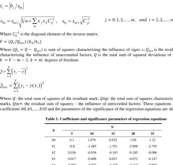
The parameters of the regression equation are calculated by the Equation 33: bj C Aij ij b y b x b x i n m m
-1 , 0 1 1 1 (33) Where C is the coefficient matrix for the unknown parameters b0, b1, ..., b25; 𝐶−1: is inverse matrix C; Cij is the elementat the intersection of the i-th row and the j-th column of the matrix 𝐶−1; n is the number of equations in the system or rows in the matrix C; 𝑦̅ is the average value of the resulting attribute y; Аij is expression
x yij i Vx y j m i V j
1 1 2 ( , , , ) (34) The residual dispersion estimate 𝜎𝑂𝐶𝑇2 is:
s y y x V m ост i i i V 2 2 1 1
( ) (35)Where yi is the deviation of the maximum likelihood estimate of the parameter of the distribution function, calculated
estimate deviation calculated by the regression equation.
The calculation of the statistics t and F to assess the significance of the coefficients of the regression equation and the regression equation as a whole is carried out according to the Equations 36-37:
t
i
b s
j bj (36)s
bos
n
x x C
j k ijs
s
C
m bj jj
ост
-1
ост -11
,
𝑗 = 0, 1, 2, . . . , 𝑚. 𝑎𝑛𝑑 𝑖 = 1, 2, . . . , 𝑛. (37)Where 𝐶𝑗𝑗−1 is the diagonal element of the inverse matrix.
𝐹 = (𝑄1/𝑄ост)(𝑘2/𝑘1) (38) Where (𝑄1 = 𝑄 − 𝑄ост) is sum of squares characterizing the influence of signs x; 𝑄остis the residual sum of squares characterizing the influence of unaccounted factors; 𝑄is the total sum of squared deviations of the resultant mark;
𝑘 =𝑉 − 𝑚 − 1, 𝑘 = 𝑚: degrees of freedom.
Q yi y i V
2 1 (39)
Q
y
iy x
i i V ост
( )
2 1 (40)Where 𝑄: the total sum of squares of the resultant mark; 𝑄пр: the total sum of squares characterizing the influence of marks, 𝑄ост: the residual sum of squares – the influence of unrecorded factors. These equations are significant. The coefficients 𝑏0, 𝑏1, … , 𝑏10 and the parameters of the significance of the regression equations are shown in Table 1.
Table 1. Coefficients and significance parameters of regression equations
b N 5 10 15 20 25 b0 0.1 1.079 0.952 1.09 1.22 b1 -0.8 -1.483 -1.551 -2.898 -2.795 b2 0.036 -0.036 -0.183 -0.185 -0.086 b3 0.017 -0.008 0.023 -0.073 -0.147 b4 -0.054 -0.077 -0.102 -0.113 -0.092 b5 0.019 0.019 -0.002 0.017 0.028 b6 -0.076 0.033 0.124 0.211 0.108 b7 0.021 0.101 0.216 0.565 0.434 b8 -0.354 -0.38 -0.219 -0.222 -0.224 b9 0.006 -0.008 0.004 0.035 0.074 b10 0.01 -0.008 -0.002 -0.045 -0.04 Q 91 164 88 284 250 Qпр 56 124 58 207 180 Qост 35 40 30 77 70
The resulting regression equations can improve the accuracy of the maximum likelihood estimate by introducing an amendment to the maximum likelihood estimate using the Equation 41:
)
(
x
y
ОМП КОН
(41)
Where λКОН is the final estimate of the distribution parameter.
Studies have evaluated the effectiveness of the constructed regression models. Another experiment was conducted to simulate the failure of equipment on a computer. Modeling samples of failures was performed according to the algorithm described above in the article. The evaluation of the effectiveness of the equations obtained was performed using newly generated random samples, and not according to those for which these equations were obtained. This proves the possibility of using the developed models for various types of equipment.
For each simulated sample were used to calculate: estimation of the maximum likelihood of the exponential distribution parameter, the corrections to the maximum likelihood estimate (30) and the final estimate of the exponential distribution parameter using expression (41).
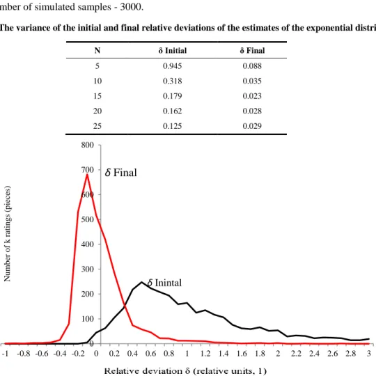
In total, 3000 samples were simulated for each experiment for each number of N sample members. The results of studies of the effectiveness of using the constructed regression equations for the exponential distribution law are shown in Table 2 and in Figures 3 to 7. The abscissa shows the relative deviations of the maximum likelihood estimates from the true value. The ordinate is the number of k estimates with a given relative deviation. The total number of estimates is equal to the number of simulated samples - 3000.
Table 2. The variance of the initial and final relative deviations of the estimates of the exponential distribution N δ Initial δ Final 5 0.945 0.088 10 0.318 0.035 15 0.179 0.023 20 0.162 0.028 25 0.125 0.029
Figure 3. Initial and final relative deviations of the estimate λ for N=5
Figure 4. The initial and final relative deviations of the estimate λ for N = 10
0 100 200 300 400 500 600 700 800 -1 -0.8 -0.6 -0.4 -0.2 0 0.2 0.4 0.6 0.8 1 1.2 1.4 1.6 1.8 2 2.2 2.4 2.6 2.8 3 N u mb er o f k r at in g s (p ie ce s) δInintal
δ
Final
0 100 200 300 400 500 600 700 800 -1 -0.8 -0.6 -0.4 -0.2 0 0.2 0.4 0.6 0.8 1 1.2 1.4 1.6 1.8 2 2.2 2.4 2.6 2.8 3 N u mb er o f k r at in g s (p ie ce s) δInitial δFinalFigure 5. Initial and final relative deviations of the estimate λ for N=15
Figure 6. Initial and final relative deviations of the estimate λ for N = 20
Figure 7. The initial and final relative deviations of the estimate λ for N = 25
0 100 200 300 400 500 600 700 800 900 1000 -1 -0.8 -0.6 -0.4 -0.2 0 0.2 0.4 0.6 0.8 1 1.2 1.4 1.6 1.8 2 2.2 2.4 2.6 2.8 3 N u mb er o f k r at in g s (p ie ce s) δInitial δ Final 0 100 200 300 400 500 600 700 800 -1 -0.8 -0.6 -0.4 -0.2 0 0.2 0.4 0.6 0.8 1 1.2 1.4 1.6 1.8 2 2.2 2.4 2.6 2.8 3 N u mb er o f k r at in g s (p ie ce s) δInitial δ Final 0 100 200 300 400 500 600 700 800 900 -1 -0.8 -0.6 -0.4 -0.2 0 0.2 0.4 0.6 0.8 1 1.2 1.4 1.6 1.8 2 2.2 2.4 2.6 2.8 3 Nu mb er o f k r at in g s (p ie ce s) δInitial δ Final
The use of the developed models significantly improves the accuracy of maximum likelihood estimates. According to Table 2, it can be seen that the variance of the relative deviations of the estimates of the exponential distribution law decreases by a factor of 4–10. At the same time, with a decrease in the number of N sample members, the efficiency of using the developed models increases. I t can be seen from Table 2 that when N is reduced from 25 to 10, the variance of the relative deviations of the maximum likelihood estimates δ initial increases by a factor of 2.5 from 0.125 to 0.318, and the variance of the relative deviations of the final estimates δ final obtained from the application of the developed technique increases very slightly from 0.029 to 0.035. In practice, when testing equipment, this will reduce the time of testing while maintaining the reliability of the calculated reliability indicators.
Software tools for the automated maintenance and repair system have been developed, which are designed to calculate the economically optimal frequency of maintenance, current and capital repairs. They automate the calculation of the optimal schedule of maintenance and repair. Their use increases the capabilities of the enterprise in self-optimizing the cost of operating electrical equipment. Software tools use the developed methodology, expand the functions of the existing system of maintenance, and repair. They should be considered and used as an addition to it.
The program allows the user to:
create and correct reference databases on equipment, types of failures and maintenance costs, current and capital repairs;
carry out operational input, adjustment and accumulation of information on maintenance, repair and equipment failures;
calculate the optimal frequency of maintenance, current and capital repairs;
carry out the output of the calculation results on the screen, printer or file;
The program consists of three modules interconnected with each other: "Directories", "Maintenance and Repair Cards", "Calculations".
The program has five directories. The “Equipment Groups” directory allows you to split all equipment in random order into groups and store the following data: equipment group code, group name. The directory "List of equipment" is designed to create a list of equipment installed at the enterprise. The following data is filled for each piece of equipment: serial number, group, name, release date, start date, start date of observation. In the "Elements of equipment" directory, the user can break each type of equipment into separate elements. Thus, it is possible to calculate the optimal frequency of maintenance and repairs, not only in general for the type of equipment, but also for its individual elements. The following data is entered in the "Equipment components" directory: equipment group, element number. Reference book "List of failures" are entered characteristics of failures: the name of the failure, the group of failure. Information on the costs associated with maintenance, repairs and overhauls, and technical diagnostics is entered in the “Cost of Repair” directory.
The second part of the program "Maintenance and Repair Cards" contains all the necessary means for entering, adjusting and storing operational information about routine maintenance in the maintenance and repair system and equipment failures.
In the third module of the "Calculations" program, calculations of the optimal frequency of maintenance, current and capital repairs, and technical diagnostics are performed.
4.
Conclusions
According to the results of the study, we can formulate the following results and conclusions.
The characteristics of samples of failures generated during operational observations or equipment tests using the [N, U, Z] plan are considered. It is shown that the samples are small, repeatedly censored on the right.
For the formation of samples of random variables according to the test plan [N, U, Z] on a computer, an algorithm was developed that ensures the adequacy of simulated samples on a computer, samples that are formed as a result of monitoring equipment.
Experimental studies were conducted to analyze the accuracy of the maximum likelihood estimates of the exponential distribution law over the formed samples of random variables. The experimental results show that the accuracy of the maximum likelihood method for N <25 is low. The relative deviation of individual maximum likelihood estimates from the true values can reach 5 or more, and half of the estimates have deviations of 0.3, depending on, the degree of censoring, the sample size.
Sampling parameters are proposed that describe its structure. All of them are measured in relative units and do not depend on the absolute values of random variables.
A computational experiment was performed on a computer to simulate samples of random variables that are adequate to samples of equipment time to failure that are formed during tests conducted according to the [N, U, Z] plan. The parameters characterizing its structure were calculated for each sample. Based on the results obtained in a computational experiment, mathematical models were constructed in the form of regression equations, establishing the relationship between the relative deviation of the estimated parameters of the studied distribution laws obtained by the maximum likelihood method and the sample parameters characterizing its structure.
A methodology has been developed for estimating the parameters of the exponential distribution law, which consists in the fact that the maximum likelihood estimates are corrected by means of corrections. Amendments to the estimates are determined using mathematical models developed in the research process.
The study of the effectiveness of the methodology for estimating the parameters of the exponential distribution law is performed. The results show that it improves the accuracy of maximum likelihood estimates of the exponential distribution law.
5.
Conflict of interest
The authors declare no conflict of interest.
6.
References
[1] Kizim, A.V. “The Developing of the Maintenance and Repair Body of Knowledge to Increasing Equipment Maintenance and Repair Organization Efficiency.” Information Resources Management Journal 29, no. 4 (October 2016): 49–64. doi:10.4018/irmj.2016100104.
[2] Baskakova N., Yakobson Z., Simaov D. The development strategy of the repair services of the enterprise. Moscow. INFRA-M (Scientific Thought), 2016.
[3] Knopik, Leszek, and Klaudiusz Migawa. “Semi-Markov System Model for Minimal Repair Maintenance.” Ekspolatacja i Niezawodnosc - Maintenance and Reliability 21, no. 2 (March 22, 2019): 256–260. doi:10.17531/ein.2019.2.9.
[4] Chang, Chin-Chih. “Optimum Preventive Maintenance Policies for Systems Subject to Random Working Times, Replacement, and Minimal Repair.” Computers & Industrial Engineering 67 (January 2014): 185–194. doi:10.1016/j.cie.2013.11.011. [5] Pham, Hoang. “Reliability of Systems with Multiple Failure Modes.” Handbook of Reliability Engineering (2006): 19–36.
doi:10.1007/1-85233-841-5_2.
[6] Esposito, Marco, Mariangela Lazoi, Antonio Margarito, and Lorenzo Quarta. “Innovating the Maintenance Repair and Overhaul Phase through Digitalization.” Aerospace 6, no. 5 (May 9, 2019): 53. doi:10.3390/aerospace6050053.
[7] Shashkin V.V., Karzov G.P. (ed.). Reliability in engineering. St. Petersburg: Polytechnic, 1992.
[8] Wakiru, J., L. Pintelon, P.N. Muchiri, and P. Chemweno. “Maintenance Optimization: Application of Remanufacturing and Repair Strategies.” Procedia CIRP 69 (2018): 899–904. doi:10.1016/j.procir.2017.11.008.
[9] Cunningham, Clair E., and Wilbert Cox. "Applied maintainability engineering." (1972).
[10] Bykhelt F., Franken P. Reliability and maintenance. Mathematic approach. Moscow: Radio and communication, (1988). [11] Barzilovich E.Yu. Models of maintenance of complex systems. Moscow: Higher School, (1982).
[12] Jenny A. Baglivo. Mathematica Laboratories for Mathematical Statistics: Emphasizing Simulation and Computer Intensive Methods. Boston College, Chestnut Hill, Massachusetts, 2005. https://doi.org/10.1137/1.9780898718416.
[13] Brimacombe, Michael. “Likelihood Methods in Biology and Ecology” (December 18, 2018). doi:10.1201/9780429143342. [14] Rasch, Dieter, and Dieter Schott. “Mathematical Statistics” New York: John Wiley & Sons Ltd (February 12, 2018).
doi:10.1002/9781119385295.
[15] Rossi, Richard J. “Mathematical Statistics” New York: John Wiley & Sons Ltd (July 18, 2018). doi:10.1002/9781118771075. [16]Young, Derek Scott. “Handbook of Regression Methods” New York: Chapman and Hall/CRC (October 3, 2018).