A Hybrid Load Flow and Event Driven Simulation Approach
for Multi-State System Reliability Evaluation
Hindolo George-Williams, Edoardo Patelli∗
Institute for Risk and Uncertainty, Chadwick Building, University of Liverpool, Peach Street, Liverpool L69 7ZF, United Kingdom
Abstract
Structural complexity of systems, coupled with their multi-state characteristics, renders their reliability and availability evaluation difficult. Notwithstanding the emergence of various techniques dedicated to complex multi-state system analysis, simulation remains the only approach applicable to realistic systems. However, most simulation algorithms are either system specific or limited to simple systems since they require enumerating all possible system states, defining the cut-sets associated with each state and monitoring their occurrence. In addition to being extremely tedious for large complex systems, state enumeration and cut-set definition require a detailed understanding of the system’s failure mechanism. In this paper, a simple and generally applicable simulation approach enhanced for multi-state systems of any topology is presented. Here, each component is defined as a Semi-Markov stochastic process and via discrete-event simulation, the operation of the system is mimicked. The principles of flow conservation are invoked to determine flow across the system for every performance level change of its components using the interior-point algorithm. This eliminates the need for cut-set definition and overcomes the limitations of existing techniques. The methodology can also be exploited to account for effects of transmission efficiency and loading restrictions of components on system reliability and performance. The principles and algorithms developed are applied to two numerical examples to demonstrate their applicability.
Keywords:
System Reliability, Event-Driven Simulation, Multi-State System, Complex System, Availability, Load-Flow
1. Introduction
A system is deemed structurally complex if it’s a non-series, non-parallel or non-series-parallel interconnec-tion of components and subsystems. Components are a system’s smallest building block and therefore deter-mine its output levels, states and behaviour. In realistic systems, these components may exist in one of several possible states/output levels [1] dictated by their fail-ure characteristics, operating conditions, age or some stochastic event outside the system boundary. The re-sult is a system characterised by multiple states, with the number of states moderated by diversity in output level of components and system structure [2, 3]. Un-like binary-state systems which can either be perfectly working or completely failed, multi-state systems can
∗
Corresponding author
Email addresses:[email protected](Hindolo George-Williams),[email protected](Edoardo Patelli)
exist in intermediate states. The number of intermediate states may or may not be finite depending on the perfor-mance measure under consideration and the type of sys-tem being studied [3]. For instance, the power generated by a hydroelectric power plant may take any value be-tween zero and its maximum achievable level depending on the height of water in the dam, the performance level of its components and demand on the grid. Other exam-ples of multi-state systems are communication systems; where data processing speed [4, 5] may be the perfor-mance measure, cooling systems; where coolant flow rate or cooling capacity [6] may be the performance measure and production systems; where production rate is the performance measure. These systems may either be standalone or form an indispensable integral part of some critical system like safety critical and industrial control systems. Therefore, it is important to be able to predict their susceptibility to failure and quantify the en-suing consequences on their performance for effective planning of preventive and corrective measures. This
process is referred to as reliability prediction. Reliabil-ity prediction has cruised through tremendous develop-ments; moving from traditional methods that consider the failure of a system as being a consequence of fail-ure of its components only to methods that treat failfail-ure of a system from a wider perspective including external factors [7]. Today, reliability prediction transcends just defining a set of standards for predicting the failure rate of components to system-level and safety of complex engineering systems [8].
1.1. Current System Reliability Evaluation Techniques In system reliability and performance evaluation, the analyst has numerous techniques at their disposal. Sometimes one technique cannot quite yield the quired outcome and a collection of techniques is re-quired instead. The technique employed is determined by the system being analysed, reliability indices of in-terest, available computing resources and the degree of precision demanded. These techniques according to [9, 10] (cited in [2]), can be classed as either heuris-tic,analytical or simulation based. They can also be classified on the basis of applicability in which case they can either bestatic ordynamic[2]. Unlike static techniques, dynamic techniques do not only model the system based on functional and structural relationships between its components but also support dynamic rela-tionships like inter component dependencies.
Reliability Block Diagrams[11, 12] and Fault Trees [11, 13] are the most common traditional reliability analysis techniques and have been used extensively in reliability evaluation of binary-state systems. Relia-bility Block Diagrams are a graphical expression of functional relationships between system components in terms of combination of functioning components re-quired for system success. Fault Trees express this functional relationship via boolean logic gates and de-pict the combination of component failure that culmi-nates into system failure. These two techniques prove particularly useful for moderately sized systems with series-parallel configurations but become cumbersome with large complex systems and often require additional techniques [14] to decompose the system. Overcom-ing this difficulty necessitated the development of Re-liability Graphs. ReRe-liability Graphs [15, 16] represent the system as a network of nodes connected by edges and they are very much efficient in modelling struc-tural complexities; system failure is defined as the non-existence of path between source and sink nodes [2]. These three techniques utilise the assumption of com-ponents being statistically independent rendering them incapacitated for systems with dynamic properties like
restrictive repairs and systems with components ex-hibiting dependent and dynamic relationships. How-ever, techniques including but not limited to Dynamic Reliability Block Diagrams [2], Dynamic Fault Trees [17], Condition-based Fault Trees [18], Dynamic Flow Graphs [19, 20], Petri Nets [21] and other combinato-rial techniques [22] have been developed to model these dynamic relationships. They have found application in a wide range of reliability engineering problems in-cluding repairable systems with restrictive maintenance policies [21, 22].
Though the earliest forms of these techniques were applicable only to binary-state systems, numerous in-stances of their recent extension to multi-state systems are present in literature. Lisnianski [23] employed an extended block diagram method to apply classical block diagram principles to a repairable system. Binary Deci-sion Diagrams (BDD) [24, 25] which underlying princi-ples are built upon Boolean algebra have also been ap-plied with success to multi-state system reliability eval-uation. They proceed via a state enumeration procedure in which each system state is represented by a multi-state fault tree. Unfortunately, multi-state enumeration is only feasible for moderately sized and simple systems, for complex systems it’s expensive and error prone if done by hand. Consequently, their applicability is limited to moderately sized simple systems. In recent years, re-liability graphs have also attracted significant attention which interest has given birth to algorithms optimized for multi-state system reliability evaluation. Though, Yeh on two separate occasions([26] and [27]) developed algorithms that do not require prior knowledge of all minimal paths or cuts of the system, most graph based algorithms do [28–31]. As such, exploiting them re-quires first deriving the desired path or cut sets using other well known algorithms which in itself is an NP-hard problem [26, 27]. Compounding their challenges (including Yeh’s algorithms in [26] and [27]) is the fact that they are based on the assumption that capacities of system components take only non-negative integer values. However, in many systems, components and system capacities are positive but not necessarily inte-ger valued. In addition to their individual short falls, the extended block diagram technique, BDD and graph based algorithms share two common limitations. They define system reliability with respect to maximum flow through the system. Therefore they are limited to sys-tems with single output nodes or syssys-tems (like signal transmission networks [32]) with multiple output nodes in which only the presence of flow at these nodes is desired but the relative magnitude is irrelevant. They stop short at solving multi-output systems with
com-peting demand at the output nodes. The second limi-tation arises from the assumption that there are no flow losses in the system, implying inapplicability to certain practical engineering systems encountered in real life in which flow under some condition (e.g. component fail-ure) escapes across the component/system boundary.
Various researchers [1, 4–6, 33, 34] have made in-valuable contributions to multi-state system reliability analysis, developing techniques applicable to a wide range of systems. These techniques are based mainly on either the structure function approach, stochastic pro-cess, simulation or the Universal Generating Function approach [3, 35, 36]. The most popular stochastic pro-cess employed in reliability analysis is Markov Chain which involves enumerating all possible states of the system and evaluating the associated state probabilities [36, 37]. This technique is only easily applicable to ex-ponential transitions or distributions with simple cumu-lative distribution functions, requires complicated math-ematics and becomes complex for large systems. The number of states in the model ranges fromm+1 for binary-state series systems to 2m for binary-state par-allel systems, where m is the number of components making up the system. For large multi-state systems, the number of states increases dramatically thereby ren-dering the model difficult to construct and expensive to compute. The Universal Generating Function(UGF) technique was introduced to address the large number of states problem the Markov Process technique is plagued with. It allows the algebraic derivation of system per-formance from the perper-formance distribution of its com-ponents [3, 38]. However, both techniques are limited in the number of reliability and performance indices they can quantify. In [39], Lisnianski introduced the Lz-Transform and inverse Lz-Transform concepts to en-hance the derivation of instantaneous reliability mea-sures like system reliability R(t), instantaneous avail-abilityA(t) and instantaneous system outputX(t) with the UGF technique [6, 38]. The UGF is a powerful tool, its applicability has been extended even to systems with dependent components as illustrated by Levitin [35, 40]. However, like the other multi-state system re-liability evaluation techniques previously discussed, the UGF is maximum flow based and assumes flow conser-vation across system components. Also, though straight forward for systems with simple series/parallel archi-tecture, it requires substantial effort for systems with a non-series/parallel structure including those composed of many subsystems. These considerations have hin-dered its application to certain multi-state system relia-bility problems.
Simulation techniques [41–43] are the most suitable
for multi-state system reliability and performance eval-uation since they mimic the actual operation of the sys-tem. Their advantages over other techniques are derived from the fact that they can support any transition distri-bution type, enhance the study of effects of external un-certainties on system performance and reliability [43] and are easily integrated with other reliability analysis techniques [44, 45]. Though computationally expensive for large systems and small failure probabilities, tech-niques that reduce the computation time and effort now exist, thanks to recent advances in computing. Variance reduction techniques and parallel computing can reduce the computation time and effort by substantial amounts when adopted. Also in extensive use are Subset Simu-lation [46] and Line Sampling [47, 48], both of which improve the efficiency of simulations. Instances of sim-ulation algorithms relying on prior knowledge of path or cut-sets are found in [43, 49, 50]. Yeh et al. [51] however developed a simulation approach that doesn’t require prior knowledge of system path/cut sets but ap-plicable only to binary-state systems.
Analytical techniques exhibit superior computational efficiency over their simulation counterparts. However, as already expressed, they suffer a setback when so-licited for realistic systems. Often, the reliability an-alyst is not only interested in steady-state or instanta-neous reliability measures but also the underlying prob-ability distributions governing the behaviour of the sys-tem as well as effects of external uncertainties (e.g., re-strictive maintenance schemes, human, environmental and other stochastic external factors) on the values as-sumed by these measures. When faced with such sce-narios, simulation becomes the most feasible alterna-tive. In summary, both analytical and simulation proce-dures are restricted by their various unique limitations. Therefore, the development of a single technique that addresses these is vital.
1.2. Proposed Approach
The proposed approach is based on the fact that if the properties of components building a system are known, then its output performance can be deduced directly from its network model. Implementing this necessitates modelling each component as a multi-state object char-acterised by a state space diagram depicting its possible states with their interactions and a set defining the prop-erties associated with each state. The operation of the system is simulated by generating component states and transition times from their state-space representation. The generated transitions are effected and the system output performance evaluated at each transition. Tran-sition and output histories of components as well as the
system are captured and saved as the simulation pro-gresses. These enhance the evaluation of any reliabil-ity/performance index both at the system and compo-nent levels. To replicate the actual operating procedure of systems, a special componentshut downandrestart operation is instituted. In this operation, the availability of each system component is tested at every transition against its predefined reference minimum input/output load level. With this, the latent interdependence of sys-tem components is accounted for.
A common feature exhibited by components of many realistic systems istransmission inefficiency; a term as-cribed to the phenomenon in which an intermediate component transmits only a fraction of flow received from its preceding component. The component in other words acts as a partial sink and dissipates part of the flow such that the flow transmitted to the next compo-nent is less than that received. Under this condition, flow is no longer conserved and techniques built around the flow conservation principle become obsolete. To illustrate the effect of this phenomenon on system re-liability, consider a 50MW power generator supplying a 45MW load through a 75MW transformer. If there are no power losses in the transformer, 45MW will be transmitted to the load. However, if the capacity of the transformer remains unchanged but its efficiency re-duces to 75%, it takes 50MW from the generator (as-suming capacity constraint is imposed) but transmits only 37.5MW to the load. In both cases, the apparent difference between capacity and demand remains con-stant but the power drawn from the generator increases and the effective power supplied to the load reduces. Other examples are a power transmission line prone to losses and an oil pipeline in which a mode of failure could be a hole in a pipe or gasket failure at some flange. The transmission inefficiency of system components may exert undesirable effects on system performance and reliability, it’s therefore worthwhile considering this property in the reliability evaluation process. In the sce-nario just discussed, the generator would need to be rated at least 60MW to match demand. Therefore, if the system is not equipped with adequate controls such that the capacity constraint is always satisfied, the genera-tor may fail due to overloading even though demand re-mains well below its rated capacity. Considering this in the proposed methodology, each component state is de-fined by an associated outputperformance levelandsink
index which respectively state the maximum flow
ac-cepted or generated and the proportion dissipated when the component resides in that state.
Convenient representation of system architecture and evaluating system output from changes in states of
com-ponents are the two prime difficulties encountered in simulation of complex multi-state systems. In the pro-posed approach, these are overcome by applying the concept of adjacency matrices from network theory to define the structure of the system. Adjacency matrices are a square array of 1’s and 0’s depicting the connec-tivity of a network and can easily represent any system architecture. They can be manipulated to obtain system flow equations which are solved to determine the mag-nitude of flow through every node of the system. The efficiency of this lies in the fact that it eliminates the need for definition of cut sets or enumeration of system states; both of which normally become laborious with complex systems. Complex network theory is a widely used concept and finds application in many engineering and real life problems. It’s particularly useful in repre-senting and analysing complexities in system structure. As a result many researchers have applied its princi-ples to a variety of problems, yielding excellent results. For instance, Dwivedi et al.[52] used it in vulnerabil-ity analysis of a power system, Todinov[53] established his optimization of repairable flow networks entirely on it and Chen et al. [54] used it to perform a reliabil-ity/availability analysis on Manhattan street networks. 1.2.1. Advantages Over Existing Techniques
The following enumerates the key contribution of the proposed technique to multi-state system reliability evaluation.
1. Being simulation based, it inherits all the advan-tages of simulation approaches to system reliabil-ity and performance evaluation. With respect to other simulation algorithms, it can implement any system structure with relative ease since it doesn’t require knowledge of minimal path or cut sets prior to system analysis.
2. It is not maximum flow based. Instead, it calculates the actual flow across every node of the system. This consequently makes possible the following; a). analysis of systems with multiple source and
sink nodes with competing demand which can be static or instantaneous
b). analysis of systems prone to losses at nodes and across edges
c). easy restart and shut-down of components so as to replicate the actual operation of systems where necessary.
3. Node capacities and system demand can take on any positive value. They do not necessarily have to be integer valued as required by graph based algo-rithms.
1.3. Outline of Paper
The remainder of this paper is organised into four sec-tions. Section 2 describes the modelling of system com-ponents followed in Section 3 by a description of how the system is modelled. The latter also contains details of the simulation procedure and its associated limita-tions. Implementation of the numerical case studies to show the applicability of the approach and an analysis of its computational requirements are contained in Sec-tion 4. SecSec-tion 5 constitutes the conclusion.
2. Component Modelling
Multi-state components and systems are discrete in space but continuous in time. That is, they exist in only one state at any given instance but reside continuously in that state until a transition occurs. The transition instan-taneously takes them to another state where they also re-side continuously until the next transition [11]. In com-ponents, these transitions are defined by time dependent probability distributions or some stochastic event out-side the component boundary which underlying proba-bility distribution may or may not be known.
Interactions between the states of annstate compo-nent and their corresponding transition probability den-sity functions can be represented by annorder square Transition Matrix, T. Sometimes certain transitions may be controlled by a direct effect of events outside the component boundary. A renown example of this would be a system composed of a series connection of multiple repairable components.
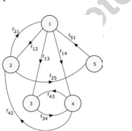
Figure 1: State space diagram of an arbitrary multi-state component
On failure of a component, the other operating com-ponents would have to be shut down and restarted only after the failed component is restored. In such a sys-tem, the shut down and restart of operating components
is triggered by the failure and repair of another compo-nent. However, the occurrence of these failure and re-pair events is marked by uncertainty, making it impos-sible to assign a probability distribution to component transitions triggered by them. Also, the triggered transi-tions may not exhibit the Markovian property, in that the component’s next state can also depend on its previous state(s). These transitions will be referred to as forced transitionssince they are induced by events outside the component boundary andnormal transitionotherwise.
If the transition from state xto yis represented by the pair (x,y) and determined by its probability density function fxy(t), then each element at position (x,y) of
T is equal to fxy(t). Assuming all possible transitions from statexhave the same priority, the next state,y de-pends only on which transition occurs first. Hence, T
completely defines the stochastic behaviour of the com-ponent as outlined in Equation 1.
T={fxy(t)}n×n|x,y (x,y)∈ {1,2, ...,n} T(x,y)=
∞, If (x,y) is a forced transition 0, If no transition between x & y
fxy(t), Otherwise
(1) Figure 1 shows the state space diagram of an arbitrary five-state component, where the label beside each arc represents the probability density function of the transi-tion depicted.
The performance level; cx of a binary-state compo-nent in statexis such thatcx∈ {0,cmax}wherecx=cmax if the component is working and0otherwise. For multi-state components, the performance level is defined by the set 0≤cx≤cmax, wherecmaxis its maximum perfor-mance level. Each state is characterised by a maximum value of load;cxthe component can supply or transmit and is referred to as its capacity in that state. There-fore, the performance of a component is defined by the vector,Cof state capacities as follows,
C={cx}n|0≤cx≤cmax, n≥2 (2) Thesink index;εxis introduced to define the amount of flow dissipated in the component in statexas a fraction of the total flow received. Applicable only to interme-diate components, this property of the component takes a value between 0 and 1. A value of 0 meaning outflow is equal to inflow and a value of 1 corresponding to the case when outflow is zero but inflow greater than zero. At a value of 1, the component effectively becomes a sink, which explains the choice of name for this prop-erty. The sink index of a component is expressed by the
vectorS,
S={εx}n|0≤εx≤1 (3) Also, a component may be subjected to loading restric-tions in a bid to preserve its reliability and/or ensure its safe operation. This often requires the load to exceed a threshold value but lie within the maximum load rating of the component. Outside this range, the component is either shut down or considered failed. The maximum load rating corresponds to the maximum value ofCbut the threshold load rating may be greater than its mini-mum value since the component may be prone to com-plete failures or maintenance states characterised by a cx value of 0. Therefore, the minimum load rating of the component is defined byΛ|0≤Λ≤cmax.
Each parameter discussed uniquely identifies a com-ponent, determines its behaviour and subsequently its effect on system performance and reliability. Therefore, a component is represented by the quintuple;E, defined as,
E=(T,C,S,Λ,x0) (4)
Wherex0is the initial state of the component.
2.1. Application to Repairable Multi-state Components and Systems
A simple illustration will be used to describe the modelling of a multi-state component with one or more repairable partial failure modes. Consider a 40MVA generator subjected to a 20% minimum load restriction and assume it generally exists in three possible states defined as follows;
• State 1, depicting operation at its nominal output level
• State 2, depicting operation below its nominal level, say 25MVA as a consequence of its partial failure
• State 3, depicting its total failure.
Presented in Figure 2 is a representation of the interac-tions between the states of the generator. State 2 is the state of interest in this illustration and the objective is to explore the possible events embedded in the restoration process frompartial failure(i.e, transition (2,1)). The figure is based on the assumption that the genera-tor remains in operation whilst undergoing repairs from state 2 (on-line repairs). However, this is not the case for components of many real world engineering sys-tems. Most components would need to be taken out of operation before repair actions can be completed. This event may also trigger the unavailability of other
components of the system as explained in the preced-ing section. Therefore, the assumption may result in over/under estimation of certain reliability indices when wrongly applied.
Now, consider the assumption that the generator is in series with an external breaker which can undergo fail-ure and repair and a further assumption that the former cannot be repaired on-line. To account for the period when it is out of operation as a result of failure of the breaker, a new state; 5 is introduced as shown in Figure 3. The restoration of the generator from state 2 to 1 may follow one of two possible operational principles;
• Case 1: Repair is initiated as soon as it enters state 2. This technically means the generator does not exist in states 2 and 3
• Case 2: Repair is delayed until the generator is not in operation i.e., either totally failed or when shut down from partial failure.
Figure 2: State space diagram of 40MVA generator
(a) Immediate repair (b) Repair only after shut down
Figure 3: Alternative state representation of generator
These necessitate the introduction of a fifth state; 4 to account for the period when it is undergoing repairs from state 2 to 1. The new state-space representations of the generator are presented in Figure 3 showing normal and forced transitions. Forced transitions would have to
be manually effected during the simulation as they do not always only depend on the current state of the com-ponent. For instance, the generator goes to state 4 from state 5 if its previous state is state 2 else it goes to state 1 as shown in Figure 3b. Using case 2 as example, the parameters of the generator would be as given below,
T= 0 f12(t) 0 0 ∞ 0 0 f23(t) 0 ∞ f31(t) f32(t) 0 0 0 f41(t) 0 0 0 0 ∞ 0 0 ∞ 0 C= 40 25 0 0 0 Λ =8
The sink index for each state is zero since the genera-tor is a source. As a rule-of-thumb, sink-index is not required for sources and sinks of a system as evident in the system flow equations derived in Section 3.2.1.
The modelling technique described can be extended to components with multiple partial failure modes. This is achieved by introducing two states (one each for shut down and repair ) for each partial failure state as shown in Figure 3.
2.2. Determining Component State Transition Parame-ters
The key to reliability evaluation of systems composed of multi-state components is being able to correctly de-termine the next state of a component and when the tran-sition takes place. The proposed algorithm for sampling the next transition parameters (next state and transition time) of a multi-state component is based on the as-sumption that the next state of the component depends on only its current state. Starting with the component in statexat timetc, the algorithm is summarised as fol-lows;
Step 1. Locate all non-zero elements in rowxofT, sav-ing their associated column number.
Step 2. Sample each element in step 1 and save the sampled value. Deterministic elements do not need to be sampled. For instance, ifT(x,y) = 10, then 10 becomes the sampled time for tran-sition (x,y).
Step 3. Find the minimum of the transition delay times obtained in step 2 and define a set containing the transitions with delay time equal to this min-imum value.
Step 4. If the set defined in step 3 has only one ele-ment, then the next state;yis the column inT
corresponding to the transition defined by the element. Otherwise, an element is randomly selected according to a uniform discrete distri-bution between 1 and the maximum number of
elements in the set. The next state is deduced from the column to which this element belongs. Step 5. The next transition time of the component is the sum of the minimum time obtained in step 3 and the current simulation time.
Algorithm 1Sampling procedure for transition param-eters of a multi-state component
Require: xandtc are respectively the current state of the component and current simulation time
functionSample(x,T,tc)
Y← f ind(T(x,:)>0).possible transitions from state x
f ←T(x,Y) .Transition Distributions k←Number of elements in f
forn←1 to kdo.Loop over number of elements Delay(n)←Sample from f(n)
end for
S ampledT ime←min(Delay) .get least delay
p← f ind(Delay←S ampledT ime) .get
transitions with Delay times equal toS ampledT ime
iflength of p>1then .Check length of p u←rand() .Generate a uniform random number between 0 and 1
index← du∗numel(p)e .Product
ofuand the length ofpapproximated to the smallest following integer
else
index← p
end if
y←Y(index) .get next component state
NextT ransitionT ime←S ampledT ime+tc
return(y,NextT ransitionT ime)
end function
These steps are summarised as a pseudo-code by Al-gorithm 1. Its major advantage is that it ensures an unbiased determination of the transition parameters of components including those exhibiting both determinis-tic and probabilisdeterminis-tic state transitions. It’s clear the al-gorithm will never select a forced transition over one exhibiting markovian properties. As a rule-of-thumb, it is not applied when the component resides in states from which onlyforced transitionsare possible (e.g, state 5 in Figure 3). The simulation algorithm should therefore be equipped with special routines to force these transitions.
3. System Modelling
In complex network theory, system topology is de-fined by a graph, which is a set of nodes connected by edges or links across which some controlled informa-tion is transmitted. This controlled informainforma-tion may be the current flowing in a circuit, energy generated from a power plant, liquid pumped from a reservoir, traffic flow rate in a street network or any quantifiable quantity of interest. In a graph, there is a set,sof nodes generating the controlled information and another set,tconsuming or utilising the generated information. Nodes belonging tosaresource nodesand nodes belonging tot;sink or target nodes. Between these two are nodes helping in transmission of the controlled information and facilitate communication between source and sink nodes. These are called intermediate nodes. The success and qual-ity of the communication process is influenced by the performance of source and intermediate nodes. If in-formation can flow in only one direction through every edge, then the graph is said to bedirectedotherwise it’s undirected or bidirectional.
3.1. The System as a Directed Graph
As already established in section 1, Engineering sys-tems are designed to accomplish a specific often quan-tifiable process. Process flow may be possible in any direction depending on the connectivity of the system and properties of its components but at any given time, its direction is known and fixed [52]. Systems are com-posed of a collection of components performing diff er-ent but specific roles and together determine the success of the process. Some of these components are respon-sible for initiating the process whilst some only serve as links to ensure progression of the process. There’s also another actor normally external to the system that utilises the process and drives it through the system. The set of components initiating the process are analogous to sources in a graph, so are the components serving as links analogous to intermediate nodes and the external factor driving the process analogous to sinks. Hence, the topology of the system can be conveniently and ac-curately represented by a directed graph.
Since the aim in system reliability evaluation is to investigate the effects of component failure on system performance and life span, the structure of the system can be represented by a directed graph with components and output points being considered nodes connected by perfectly reliable edges i.e., edges do not fail. When modelling systems with unreliable links e.g, power dis-tribution networks, then each unreliable link should be treated as a component and represented as a node. IfG
is a directed graph, then the structure of the system is defined byGas,
G=(V,A) (5)
whereVis the set of nodes andA, the adjacency ma-trix. The adjacency matrix is anMorder square matrix defining the connectivity of nodes, whereMis the total number of nodes of the system . A connection between nodeiandjin the system is represented in the adjacency matrix by 1 at the intersection of rowiand columnjif process flow is from nodeitoj(i → j), 1 at the inter-section of rowjand columniif flow is from nodejtoi (i ← j) and 0 if a connection does not exist. The node pair, (i,j) representing a connection and flow from node itojis known as an edge,ei j of the system. A row of the adjacency matrix depicts the source node of an edge and a column; the incident/target node of the edge. The edges of the system are defined by akby 2 matrix; e, wherekthe total number of edges is equal to the sum of the elements of the adjacency matrix.
A={ai j}M×M|ai j = 1 If flow isi→ j 0 Otherwise (6) e={i,j}k×2|k= M X j=1 M X i=1 ai j ∀(i,j)∈V (7) For some systems, the links may be reliable but inef-ficient which can have negative effects on system relia-bility and performance. Letαi jbe the efficiency of edge ei jsuch that 0< αi j≤1. Note that if the efficiency of a link is zero, then it becomes a sink and should therefore be treated as a node. If in defining the adjacency ma-trix, the efficiencies of the links are used, then Equation 6 becomes; A={ai j}M×M|ai j= αi j If flow isi→ j 0 Otherwise (8)
andkredefined as the total number of non-zero elements of A i.e., k = PM
j=1
PM
i=1(ai j > 0). Another property of links encountered in many real world systems (e.g, transmission lines in power distribution systems) is their maximum load rating. Let li j be the maximum allow-able load for edgeei jsuch that 0<li j ≤ ∞. The upper bound corresponds to the case when no load restrictions are imposed on the edge. Though unrealistic, this as-sumption is useful in maximum flow analysis of distri-bution networks. To account for this third property of a network, thecapacity matrix;Lis introduced to define the maximum capacity of edges. Each non-zero element of Lcorresponds to a non-zero entry inA.
Therefore, Equation 5 can be adapted to define both the structure of a system and the properties of its links as expressed in Equation 10.
G=(V,A,L) (10)
Now that the adjacency and edge matrices have been discussed and their mathematical relations expressed, a fourth matrix defining the relationship between edges and nodes of the system with respect to the direction of process flow will be introduced. This matrix is known as the incidence matrix;Γand is anMbykmatrix with nodes represented by rows and edges by columns. If the edges are numbered from 1 tokand nodes from 1 toM, then for an edgeei j, the element in the column corresponding to the edge number (i.e., index of (i,j) in matrixe) and rowi(the local source node), is assigned the value 1, the element in rowj(the incident/local tar-get node) is assigned the value−ai j and 0 in all other rows. Γ={γpq}M×k|γpq= 1, p=i −ai j, p= j 0, otherwise ∀(i,j)∈e (11)
The variableq =1,2, ...,k(the edge number) is the in-dex of edge (i,j) orei j ineandp =1,2, ...,M. Given the adjacency matrix alone of the system,eandΓcan be derived by applying equations 7 and 11. This procedure is summarised in Algorithm 2.
3.2. System Representation and Flow Analysis
As discussed in section 3.1, a system can be repre-sented by a directed graph comprising source, interme-diate and sink nodes. The source and intermeinterme-diate nodes are physical components making up the structure of the system while sink nodes are output points via which system output is consumed. All three node types can be modelled by the methodology proposed in section 2. However,Tis usually unknown for output nodes prior to analysis can therefore not be defined. Also,Sis not required for output/sink nodes as evidenced in the sys-tem flow equations derived later in Section 3.2.1. There-fore, for output nodes, equation 4 could be re-written as,
E=(C,Λ) (12)
Since it’s impossible to determine all output levels prior to analysis for some systems, specifying C for sink/output nodes is optional. Alternatively, it could be defined by specifying only the output levels of interest.
Algorithm 2Procedure for deriving theedgeand in-cidencematrices of a system
Require: A, the adjacency matrix of the system
functionGetMatrix(A)
M ←size(A,1) .get number of nodes
k←PM
j=1
PM
i=1(ai j>0) .get number of edges
forn←1 to Mdo
index←columns with non-zero entries w←number of elements inindex
e(end+1 :end+w,:)←[n∗ {1}w×1 indexT]
end for
Γ← {0}M×k .predefine the incidence matrix by anMbykarray of zeros
i←vector of elements in column 1 ofe
j←vector of elements in column 2 ofe
position← jT+{0,1, ...,k−1} ∗M position1←i+(j−1)∗M
Γ(position)← −A(position1) .update values position2←iT +{0,1, ...,k−1} ∗M
Γ(position2)←1 .update values
return(e,Γ)
end function
IfEis the set containing the properties,Eiof each node of the system, then the system structure and property can be defined by the setS.
S=(G,E)|E={Ei}M ∀i∈ {1,2, ...,M} (13)
3.2.1. Derivation of System Flow Equations
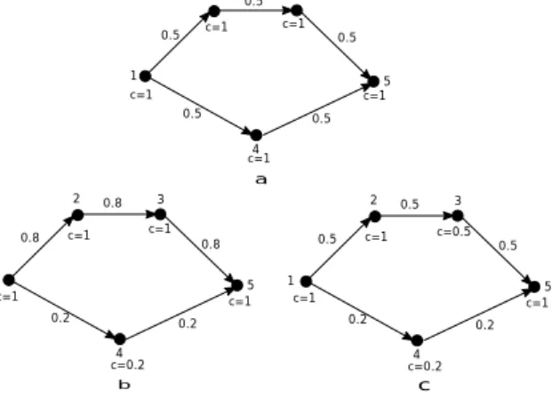
To understand the flow of processes in systems, it’s worthwhile to think of source nodes as reservoirs and intermediate nodes as valves in a pipe network. The total flow through the system depends on the amount of liquid in the reservoir and the resistance to flow in the pipe network. These properties are functions of the capacities of the source and intermediate nodes respec-tively. As source and intermediate nodes perform their functions, their capacities change consistent with their state-space diagrams, leading to a change in resistance of some flow paths. The result is the existence of paths with high resistance and some with very low resistance triggering differential flow redirection. The amount of flow through a path is directly proportional to the capac-ity of the smallest node in that path. Hence, more flow will be redirected through the path of least resistance (highest capacity) as illustrated in figure 4.
Node 1 is a source, node 5 a sink and nodes 2, 3 & 4 are intermediate nodes. Initially, all intermediate nodes have the same capacity, resulting in equal path
resis-tance for both upper and lower paths between source and sink. Hence, the 1 unit of flow from the source is split equally between the paths as shown in Figure 4a. In Figure 4b, the capacity of node 4 reduces to 0.2 thereby creating a difference in resistances of the two paths. Since the maximum capacity of the upper path is 1, 0.8 units of flow are redirected through it and 0.2 through the lower path. If at this stage, the capacity of node 3 is also reduced to 0.5 (Figure 4c), the capacity of the upper path becomes 0.5. Therefore, only 0.5 units of flow are transmitted along the upper path and 0.2 along the lower. 1 2 3 4 5 2 3 4 5 c=1 c=1 c=1 c=1 c=1 0.5 0.5 0.5 0.5 0.5 c=1 c=1 c=0.2 c=1 c=1 0.8 0.8 0.8 0.2 0.2 2 3 4 5 c=1 c=1 c=0.2 c=1 c=0.5 0.5 0.5 0.5 0.2 0.2 a b c 1 1
Figure 4: Flow visualisation in an arbitrary 5 node system
Flow redirection may appear simple and straight for-ward for systems as simple as the one shown in Figure 4 but presents itself as an optimization problem for large systems with complex topology. The optimization nor-mally consists of multiple parameters and constraints and has as its goal the calculation of flow along each edge of the network.
LetXi j be the magnitude of flow in edgeei j,f+i; the set of nodes connected to the inlet of nodei, f−i; the set of nodes connected to the outlet of nodei,c{xi}; the current capacity of node i and x; the current state of nodei. The total inflow for source nodes is zero and for sink nodes, the total outflow is zero which meansi ∈ s iff+i = ∅andi ∈ t iff
−
i = ∅. The constraints and by extension the equations governing the optimization procedure hinge on the following assumptions;
1. The system is equipped with adequate controls such that flow does not exceed the capacity of a node. This is known as the capacity constraint. For intermediate and sink nodes, it means the total in-flow should not exceed the node capacity and it’s
expressed mathematically as,
X
j∈f+i
Xjiαji≤c{xi} |(i,j)∈e, f+i ⊂V (14) For source nodes, the statement means the total outflow should not exceed the node capacity;
X
j∈f−i
Xi j≤c{xi}|(i,j)∈e, f
−
i ⊂V (15)
Equations 14 and 15 can be combined into a single equation defining the capacity constraint of all the nodes of the system.
Θ{Xi j}k×1 ≤ {c{xi}}M×1 |(i,j)∈e, ∀i∈V (16) The matrix,Θis related to the incidence matrix,Γ of the system as follows,
Θ={θiq}M×k|θiq= γiq, i∈s −γiq, γiq<0 0, otherwise (17)
2. Flow in the system is conserved. That is,
• Total flow generated by sources equals the sum of flow consumed by sinks and any losses at intermediate nodes.
• The total inflow at an intermediate node; i |
i ∈ (s∪t)0 equals its total outflow plus any losses at the node.
Expressing the second statement mathematically, equation 18 is obtained; X j∈f−i Xi j− X j∈f+i Xjiαji=0|(i,j)∈e (18)
The flow conservation constraint equation for the system can be obtained by applying equation 18 to all intermediate nodes of the system. This equation is defined as,
Φ{Xi j}k×1={0}ð×1 ∀(i,j)∈e (19)
whereð is the number of intermediate nodes. If
the incidence matrix,Γis expressed in terms of its rows,Γpi.e., Γ= Γ1 Γ2 . . . ΓM−1 ΓM ={Γp}M |p=1,2, ...,M (20)
thenΦandΓare related as expressed in equation 21. Φ= Φ1 Φ2 . . . Φð−1 Φð ={Φλ}ð|Φ λ= Γp, λ=1,2, ...,ð ð<M, f :λ→p ∀p∈(s∪t)0 (21) In other words, Φ (row designated asΦλ) is a ð
byksub matrix ofΓcontaining all the rows inΓ corresponding to intermediate nodes.
If the transmission efficiency of intermediate nodes is considered, and given thatε{xi}is the current sink index of nodei, equation 18 is rewritten as,
X j∈f−i Xi j−(1−ε{xi}) X j∈f−i Xjiαji=0|(i,j)∈e (22)
and the matrix,Φin equation 19 redefined as
Φ={φλq}ð×k|φλq= (1−ε{xp})γpq, γpq<0 γpq, otherwise λ=1,2, ...,ð, ð<M f :λ→p ∀p∈(s∪t)0 (23) Comparing equations 21 and 23 reveals that the former is a special case of the latter which is the case when the value ofε{xi} is set to 0 (i.e., 100% efficient nodes).
3. If the capacity of a node changes, the flow in the system is reconfigured to match the prevailing sys-tem conditions. The flow,Ψ, generated by sources is such that flow into sinks is maximised. That is, sources always try to match available demand. For a system,Ψis defined as,
Ψ=−X j∈f−i X i∈s Xi j =−{ψq}1×k{Xi j}k×1|ψq= X i∈s γiq q=1,2, ...,k (24)
In the optimization problem, the goal is to deter-mine the minimum value ofΨthat maximises the flow in the system. Hence,Ψrepresents the objec-tive function of the optimization.
4. The minimum allowable flow through an edgeei j is 0 but the maximum is defined by the smallest of the maximum capacities of its nodesi&jand its capacity; li j. That is, 0 ≤ Xi j ≤ Ωi j, where
Ωi j is the maximum flow through the edge. Iflb represents the vector of lower bounds and ubthe vector of upper bounds of all edges of the network, then, lb={0}k×1, ub={Ωi j}k×1 Ωi j =min{c{maxi} ,c {j} max,li j} ∀(i,j)∈e (25)
Equations 16, 19, 24 and 25 form the basis of the op-timization process which can be implemented by a va-riety of well known algorithms. However, the numer-ical examples presented in this paper are based on the interior-point algorithm [55, 56] available in Matlab’s linear programming toolbox.
So far, only unidirectional links have been consid-ered. Without loss of generality, the equations proposed remain valid for bidirectional links. Such links are nor-mally represented by two reciprocal edges i.e., edges connecting the same pair of nodes but allowing flow in opposing directions. For instance, edgese12ande21 are reciprocals. The outcome of the optimization some-times results in flow across both reciprocal edges. How-ever, since in practice both edges represent the same physical link/element and given that flow at any instance is possible in only one direction, the flows should be normalised to obtain the actual flow through the link. The actual direction of flow across the link is given by the direction of the larger flow. The magnitude of this flow is obtained by temporarily setting the capacity of the edge with the smaller flow to zero and repeating the optimization process. This is expressed in Equation 26 as; Ωgh=0|(g,h)= (j,i) IfXi j>Xji (i,j) Otherwise (26) 3.2.2. Output Calculation and Node Reconfiguration
In an engineering system, failure or change in output level of one component may lead to change in output level of other components. This change may trigger shut down of operating components or restart of components already in shut down. Therefore as components undergo their normal failure and repair cycles, the system also undergoes a series ofshut downandrestartoperations. It’s imperative that these shut down and restart opera-tions be accounted for in the simulation process for a realistic outcome as the failure of most components de-pends on the time spent in operation.
Taking a component out of operation affects all com-ponents connected to it and hence process flow in the system. Therefore, the effective output of a node after every system transition is the flow through it when the last shut down operation has been executed and there are no nodes left requiring shut down. For this reason, an iterative procedure is employed in system output cal-culation. This procedure is based on the following as-sumptions and principles,
• the availability of a node is determined by the mag-nitude of its input flow only
• a node is shut down when the flow through it is ei-ther zero or below its predefined threshold value and its current capacity is non-zero; provided a shut down state is defined in its state-space dia-gram
• nodes are shut down in descending order of their rank
• nodes with zero input flow are placed higher on the scale.
• non-zero input flow nodes are ranked in order of their degree of inadequacy (i.e percentage by which the input falls short of the threshold)
• equally ranked nodes have the same priority and are shut down randomly.
Highlighted below is the iterative procedure proposed for system output calculation.
Step 1. Calculate system flow using equations 16, 19, 24 and 25.
Step 2. Find nodes requiring shut down and rank them. Step 3. Select node at the top of the scale, save its next transition parameters, execute shut down and set its next transition time to infinity. If the in-put of the node is non zero, add it to the set
U. Add the component to the maintenance list if transition to a maintenance state from shut down is possible and provided it’s not already on the list andforce maintenance.
Step 4. Repeat step 3 until all zero input nodes have been shut down. Go to step 6 if there’s no node left to shut down.
Step 5. Repeat steps 1 to 3 until the list of components to shut down is exhausted.
Step 6. Determine state of sink nodes if necessary. This is the state number corresponding to the magni-tude of flow into the node.
The complementaryrestartoperation is carried out to restore nodes to their previous states prior to their being shut down. Enumerated below are the steps entailed. Step 1. Perform system flow optimization using
equa-tions 16, 19, 24 and 25, previous sink indices and previous capacities of nodes before they were shut down.
Step 2. Select a node in shut down.
Step 3. Check if its input flow exceeds its threshold flow.
Step 4. If it does, determine how long it took in shut down.
Step 5. Restore node to its previous state and update its next failure time and state. Remove component from maintenance list if it’s repairable only in shut down. Also remove component fromUif applicable.
Next Failure Time =(Failure time before shut down)+(time spent in shut down)
Step 6. Repeat steps 2 to 5 until all nodes in shut down have been looped through. Go to step 8 ifUis empty.
Step 7. Set to zero the current capacities of components inUand repeat steps 1 to 6.
Step 8. End procedure 3.3. Simulation Procedure
Summarised below are generic systematic steps pro-posed for simulation of structurally static homogeneous time dependent systems.
Step 1. Initialise system in preparation for simulation. This involves the following,
a). initialization of vectors to save the current capacities; {c{i}}M×1, current sink indices;
{ε{i}}M×1, next transition times;
τ | τ ={τi}M×1 as well as state and output histories of nodes
b). setting the required number of simulations (N samples), mission time (Tm)
Step 2. Set the simulation time; t = 0, U = ∅, sam-ple the next transition parameters of nodes and updateτ.
Step 3. Determine initial state of sink nodes and carry out any necessary reconfigurations (including shut down and restart where necessary) Step 4. Update initial state and output history of nodes Step 5. Set the current simulation time to the minimum
ofτ. That is,t=min(τ).
Step 6. Check for nodes with next transition time equal toti.e.,τi=tand for each node,i,
a). effect the required transition and sample its next transition parameters
b). update τ, {c{i}}M×1, {ε{i}}M×1 and its state history
c). add component to maintenance list if new state is a maintenance state or if transition to a maintenance state from new state is possible.
Step 7. For each component on the maintenance list, force maintenance.
Step 8. Compare previous and current values of
{c{i}}M×1 and {ε{i}}
M×1. If a difference is ob-served in at least one of the two vectors, a). restart any nodes in shut down b). determine the new value of matrixΦ c). calculate system flow and shut down nodes
via the procedure described in section 3.2.2 using the new values of Φ, {c{i}}M×1 and
{ε{i}}
M×1. Note that all other parameters of equations 16, 19, 24 and 25 remain static throughout the simulation
d). for each node of the system, update output history if new output is different from out-put at previous transition.
Step 9. Repeat steps 5 to 8 untilt = Tm, updating τ,
{c{i}}M×1,{ε{i}}M×1and node state & output his-tories at every transition.
Step 10. Repeat steps 2 to 9 for the desired number of times, saving node histories at each trial. From the state and output histories of nodes, desired reliability and performance indices can be obtained us-ing standard statistical analyses and the basic definition of the index of interest. These fall outside the scope of this paper but details can be found in [57].
Indices such as failure distribution, failure frequency, reliability function, average availability, instantaneous availability, instantaneous output, state probabilities, ca-pacity factor and actual distributions of transitions with unknown distributions prior to the analysis are all ob-tainable from the state and output histories of nodes.
State duration based simulation technique achieves superior accuracy relative to the standard sequential Monte Carlo simulation described in [41] when applied to repairable systems. The upper hand is due to the in-corporation ofshut downandrestartof nodes as a con-sequence of the behaviour of other system nodes. The standard technique on the other hand assumes statistical independence of system nodes.
3.4. Limitations
The proposed simulation procedure is challenged by two major limitations. The first is consequent of the
assumptions used forshut down andrestart of nodes. That is, the availability of a node is determined by the magnitude of its input flow only. This restricts the ap-plicability of the methodology to homogeneous and in-dependent heterogeneous systems. However, it can be easily extended to interdependent systems by incorpo-rating fault trees and redefining the conditions forshut downandrestart.
Also, the capacity constraint imposed on source and intermediate nodes means the effects of Common Cause Failures (CCF) resulting from flow redistribution cannot be studied. However, the procedure can be used in sys-tem design to estimate the required syssys-tem parameter values to prevent these failures.
4. Case Studies
The principles and algorithms derived and described in the preceding sections were translated into a Matlab based application and applied to two case studies. The random variable generator available in the open source uncertainty quantification tool, OpenCossan [58]; de-veloped at the Institute for Risk and Uncertainty of the University of Liverpool was incorporated to enhance sampling from any probability distribution including user-defined distributions.
4.1. Case Study 1: A Simple Pipe Network
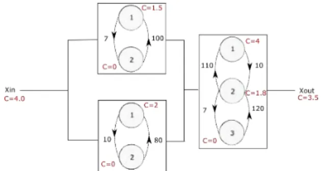
Figure 5: Structure of pipe network
Shown in Figure 5 is an oil transmission line showing the state-space representation of each component and was originally presented as Example 2.4 in [36]. Indi-cated beside each arc is the transition rate (in transitions per year) and beside each state number; the capacity (in tons of oil flow) of the component in that state. Flow is from left to right and the demand at Xout is conserva-tively assumed to be at 3.5 tons since this is the maxi-mum possible flow through the network.
4.1.1. Analyses
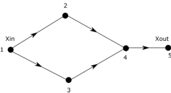
The structure of the system can be represented by a network of 5 nodes. Numbering these chronologically from left to right, the network model is as given in Fig-ure 6.
Figure 6: Network model of pipe network
Given that the efficiency and capacity of the links are of no interest in the analysis, the links are assumed to be 100% efficient and the adjacency matrix becomes;
A= 0 1 1 0 0 0 0 0 1 0 0 0 0 1 0 0 0 0 0 1 0 0 0 0 0
FromA,eandΓcan be obtained using Algorithm 2 as;
e= 1 2 1 3 2 4 3 4 4 5 Γ= 1 1 0 0 0 −1 0 1 0 0 0 −1 0 1 0 0 0 −1 −1 1 0 0 0 0 −1
Applying the procedures described in Section 3.2.1, the parameters of the flow equations are obtained as;
Θ= 1 1 0 0 0 1 0 0 0 0 0 1 0 0 0 0 0 1 1 0 0 0 0 0 1 ub= 1.5 2 1.5 2 3.5 Φ= −1 0 1 0 0 0 −1 0 1 0 0 0 −1 −1 1
The objective function,Ψis;
Ψ= −1 −1 0 0 0 X12 X13 X24 X34 X45
(a) Nodes 2 & 3 in all 3 cases
(b) Node 4 in Case 2
(c) Node 4 in Case 3
Figure 7: State-space diagram of components
Note: CM represents corrective maintenance state. The problem under review was solved by Lisnianski et al.[36] using Markov Chain and assuming on-line re-pairs to node 4. This was repeated using the technique described in this paper and the analysis taken further by considering two other possible operating principles that can be imposed on the system. These are summarised as,
1. Assuming on-line repairs to node 4.
2. Node 4 is taken out of operation during repairs and these repairs commence almost instantaneously as the node enters a degraded state.
3. Node 4 is taken out of operation during repairs but a repair action only commences after the compo-nent is shut down as a result of failure of other nodes.
The system was analysed for these 3 cases and the re-sults compared to bring out the effects of the various assumptions on the reliability and performance indices of the system. Figure 7 shows the state-space diagrams of all 3 components modelled as described in Section 2.1.
4.1.2. Results and Comments
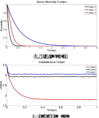
For a mission time of 4 years and 20000 samples, the reliability and performance indices of the system ob-tained from the simulation are presented in Figure 8.
(a) Reliability function
(b) Instantaneous Output
Figure 8: System reliability and performance indices
Though this case study involves a simple system, it presents an irrefutable illustration of the effects of com-ponent modelling error on accurate estimation of system reliability and performance indices. As shown in Figure 8, modelling node 4 according to the assumptions made in case 1 would result in over estimation of system reli-ability and output if the system were operated according to case 2 or 3.
4.2. Case Study 2: A Multi-State Bridge Network Bridge networks are a typical example of structural complexity exhibited by engineering systems. Reliabil-ity analysis of even the simplest bridge network is cum-bersome when compared to analysis of a similarly sized system with a non-bridge configuration.
To show the applicability of the methodology devel-oped, the imaginary multi-output, non-repairable com-plex bridge network shown in Figure 9 is considered. In the network, nodes 1, 2 and 3 respectively designated S1, S2 andS3 are sources while nodes 4, 5 and 6 are sinks respectively labelledXout1,Xout2andXout3. The source nodes have identical failure characteristics but the capacity ofS1is 1.5 times the individual capacities of the other sources. Also, the demand at node 6(70 units) is twice the individual demands at nodes 4 and 5. In addition, all diagonal links in the network are unidi-rectional with flow from left to right.
1 2 3 4 5 6 7 8 9 10 11 12 13 14 15 16 17 18 19 20 21
Figure 9: Block diagram of test bridge network
Figure 10: State space diagram of nodes (a)Source nodes (b)Intermediate nodes(c) Nodes 14-20 for case 3
4.2.1. Analyses
The intermediate nodes, according to their position in the system and similarity in failure characteristics are grouped and arbitrarily designated as follows,
a). nodes 7 to 13 and node 21 will be referred to as central nodes
b). nodes 14 to 16, referred to as vertical bridge nodes and
c). nodes 17 to 20, referred to as horizontal bridge nodes
Shown in Figure 10 are the state space diagrams of the nodes of the system as modelled by the procedure de-scribed in Section 2.1.W,PF,FandSrespectively rep-resentWorking; depicting the operation of a node at its expected level,partial failure; when the node operates below its expected level,Failure; when the node is com-pletely failed andShut down; when the node is taken out of operation but not as result of failure. The network was analysed for three cases;
1. when flow through components 17 to 20 is from left to right only but components 14 to 16 are bidi-rectional
2. when components 14 to 20 are bidirectional 3. when components 14 to 20 are bidirectional and
have a failure state in which their capacity remains unchanged but efficiency reduces by 20%.
60 40 40 70 70 70 35 35 35 70 35 35 35 70 35 70 35 35 70 35 35 35 70 35 35 35 35 35 35 35 35 35 35 70 S1 S2 S3 Xout1 Xout2 Xout3 7 8 9 10 11 12 13 14 15 16 17 18 19 20 21
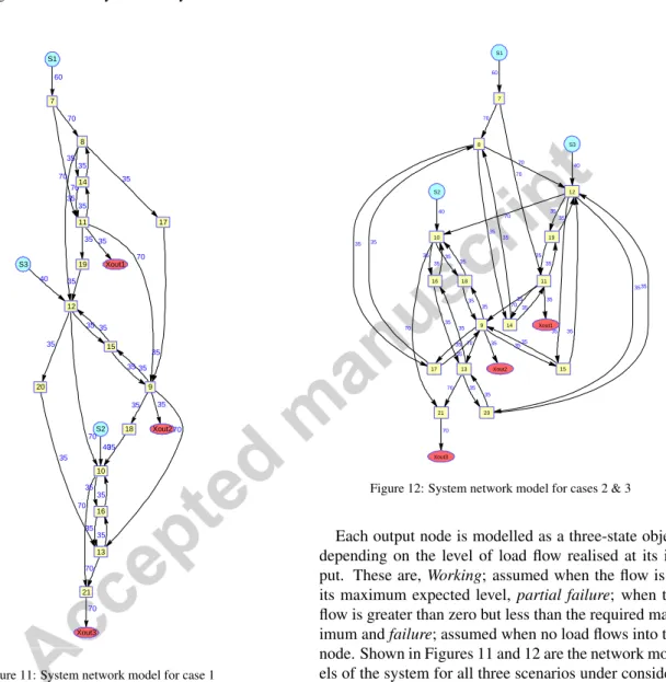
Figure 11: System network model for case 1
The properties and failure characteristics of the com-ponents of the system are presented in Table 1. E xp(a) represents an exponential distribution of mean a, LN(a,b); a Log-Normal distribution of meana and standard deviationbandW(a,b); a Weibull distribution with parametersa andb. It should be noted that the same component failure characteristics are used in all three cases.
Table 1: Node properties
Node Type Transition Distribution Capacity 1-2 Exp(10) S1 1-3 LN(20,2) 60 45 0 0 2-3 LN(4.5,1.2) Central Nodes 1-2 LN(15,3) 70 0 0 Bridge Nodes 1-2 W(12,2) 35 0 0 60 40 40 70 70 70 35 35 35 70 35 35 35 35 35 70 35 70 35 35 70 35 35 35 35 35 70 35 35 35 35 35 35 35 35 35 35 35 35 35 35 70 S1 S2 S3 Xout1 Xout2 Xout3 7 8 9 10 11 12 13 14 15 16 17 18 19 20 21
Figure 12: System network model for cases 2 & 3
Each output node is modelled as a three-state object depending on the level of load flow realised at its in-put. These are, Working; assumed when the flow is at its maximum expected level, partial failure; when the flow is greater than zero but less than the required max-imum andfailure; assumed when no load flows into the node. Shown in Figures 11 and 12 are the network mod-els of the system for all three scenarios under consider-ation with an indicconsider-ation of the maximum allowable load through each edge.
4.2.2. Results and Comments
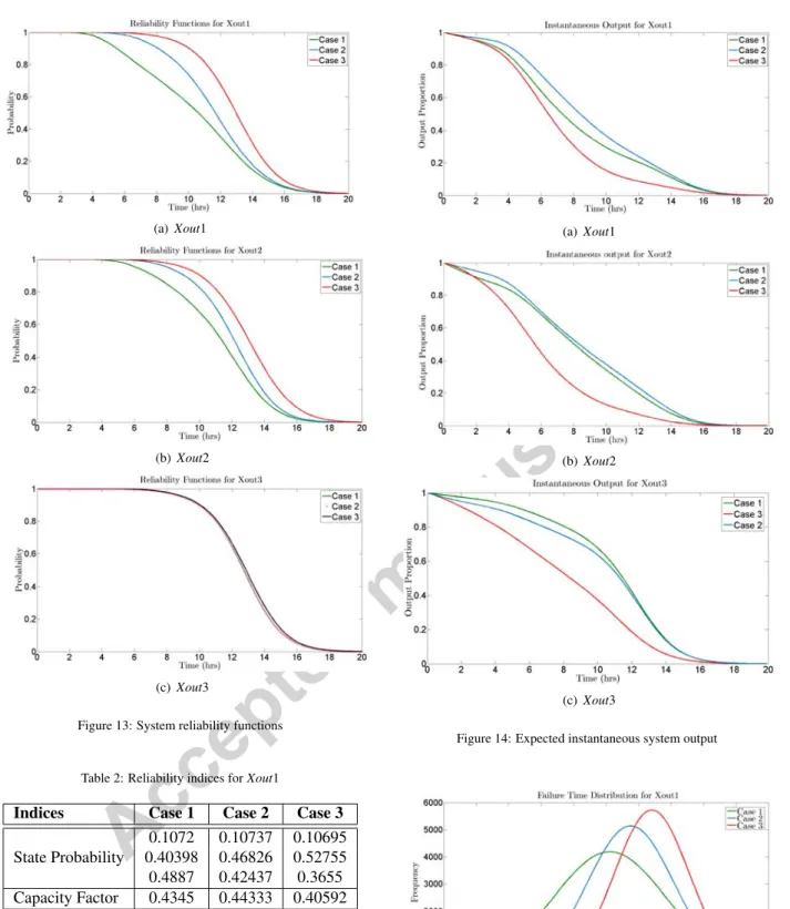
The system was simulated for a mission time of 20 hours using 60,000 samples. Presented in Table 2 is a summary of the average values of the most important reliability indices forXout1 and shown in Figure 15 are its failure time distributions.
(a)Xout1
(b) Xout2
(c)Xout3
Figure 13: System reliability functions
Table 2: Reliability indices forXout1
Indices Case 1 Case 2 Case 3
0.1072 0.10737 0.10695 State Probability 0.40398 0.46826 0.52755 0.4887 0.42437 0.3655 Capacity Factor 0.4345 0.44333 0.40592 Availability 0.5113 0.57563 0.6345 MTTF 10.2306 11.5172 12.6959 No. of Failures 0.9996 0.9996 0.9995
The expected instantaneous output and reliability functions at the three output nodes are respectively pre-sented in Figures 14 and 13. This case study was
(a) Xout1
(b)Xout2
(c) Xout3
Figure 14: Expected instantaneous system output
designed to portray the effects of system configura-tion and efficiency of components on the reliability and performance of output nodes. As evidenced in Figures 14 and 13, the performance and reliability of the system at output nodes exceptXout3 are indeed affected by the factors under consideration.
System reliability in this case study is defined with respect to complete failure i.e., zero output. Therefore a non-zero load flow at a node renders it reliable irrespec-tive of the magnitude of flow. The reliability ofXout3 remains unaffected in all three cases (see Figure 13c) because being a terminal node, the magnitude of flow realised at its inlet may change from case to case but the likelihood of the presence of this flow remains unaf-fected. The case study indicates why reliability should not be used as the only parameter to compare the re-sponse of a multi-state system under different condi-tions. It also shows that the response of an output node depends on its position in the system relative to other output nodes as well as sources.
4.3. Computational Costs Flow Calculation 80% Update Output 6% Sampling 3% Reconfiguration 5% Others 6%
(a) Case Study 1
Flow Calculation 89%
Update Output 6% Sampling 3% Others 3%
(b) Case Study 2
Figure 16: Simulation time utilisation per subroutine
Table 3: Actual computational cost per case study Case Studies
1 2
Average time per sample (s) 3.92 0.9287
Estimated total time (s) 78400 55722
Actual simulation time (s) 3163 2128.267
Improvement factor 24.79 26.18
Figure 16 shows how the total simulation time is dis-tributed among the key tasks of the algorithm. They are based on a study of 1000 samples each, of the two case studies on a48 core, 1895.257MHz AMD Opteron(tm)
6168 processor. In Table 3 is a comparison of what
the simulation times would be if run serially on a single core and the actual times spent using 24 cores running in parallel. We used 24 cores because the simulations were run on a shared facility and that was the maxi-mum allowed for a single user. The estimated time is the product of the simulation time per sample and the total number of samples (20000 and 60000 for cases 1 and 2 respectively). Ideally, the improvement factor; the ratio of estimated to actual simulation time should be slightly less than the number of parallel cores due to initializa-tion and overhead communicainitializa-tion among cores. How-ever, during parallelization, certain system initialization steps which were repeated for every sample in the se-rial simulation were carried out only once and broadcast across all 24 cores resulting in time gains.
Flow calculation, as depicted by Figure 16 accounts for the largest share of the computation time. Its magni-tude depends on the nature and size of the system (i.e., whether the system is repairable or not), mission time and total number of simulation samples. There were on average 142 calls to the flow calculation subroutine per simulation sample in case study 1 with each call last-ing 0.0221 seconds. Case study 2 had an average of 20 calls per simulation sample, each call lasting 0.0430 seconds. Incorporating variance reduction techniques resulting in less number of samples required should im-prove the time efficiency. Depending on the system, additional gains can also be derived from the complete omission of thereconfigurationsubroutine. Reconfigu-ration (shut down & restart of nodes) is unnecessary for non-repairable systems (e.g. case study 2) and systems for which components are assumed to be statistically in-dependent.
In summary, the size and degree of system activity determine the simulation time. However, as evidenced in Table 3, the 21-node non-repairable system with less activity required less simulation time than the 5-node