ECTree: An Extended Tree Index Structure for Attributed Subgraph Queries

(1)

ECTREE: AN EXTENDED TREE INDEX STRUCTURE

FOR ATTRIBUTED SUBGRAPH QUERIES

Jun Luo

A thesis in

The Department of

Computer Science and Software Engineering

Presented in Partial Fulfillment of the Requirements

For the Degree of Master of Applied Science(Software Engineering) Concordia University

Montr´eal, Qu´ebec, Canada

May 2012 Jun Luo, 2012

(2)

Concordia University

School of Graduate Studies

This is to certify that the thesis prepared

By: Jun Luo

Entitled: ECTree: An Extended Tree Index Structure for Attributed Subgraph Queries

and submitted in partial fulﬁllment of the requirements for the degree of

Master of Applied Science(Software Engineering)

complies with the regulations of this University and meets the accepted standards with respect to originality and quality.

Signed by the ﬁnal examining committee:

Chair Dr. B. Jaumard Examiner Dr. T. Eavis Examiner Dr. N. Shiri Supervisor Dr. G. Butler Approved

Chair of Department or Graduate Program Director

20

Dr. Robin A. L. Drew, Dean

(3)

Abstract

ECTree: An Extended Tree Index Structure for Attributed Subgraph

Queries

Jun Luo

Graphs are popular data structures for modeling complex data types, especially graphs with attributes for gene sequences, protein structures, chemical compounds, protein interaction networks, social networks, etc. There is a need for managing such graph data and providing eﬃcient querying tools. In the graph mining realm, the problem lies in indexing a large number of graphs for fast retrieval. Indexing at-tributed graphs and using atat-tributed queries can provide faster response time and more reﬁned results.

This thesis focuses on extending an existing index to support attributed graph indexing and providing subgraph querying access to the extended index. The aim is to find a way such that the labels of the graphs as well as the attributes of the graphs are indexed at the same time. A query format is provided to query the extended index on the attributes with flexibility which allows intervals to be used. In addition, regular expressions and label groups are used as query labels so that multiple queries that have similar structures can be combined as a single query. This also benefits in that a query graph does not have to use fixed labels. We also introduce a vertex degree-attribute based vector to capture both the features of a data graph and a query graph. A novel pruning method is proposed and implemented so that the pruning based on the degree-attribute vectors can still be adopted even when it is not clear how to define a histogram pruning for the query graphs that use non-fixed labels. All the techniques presented in our work are validated through experiments on both real and synthetic datasets.

(4)

Dedication

The completion of this thesis would not have been possible without the help of a lot of people. It is all those people who oﬀered support when I was in need that bring me this far. I would like to express my most sincere gratitude to them.

First and foremost, I want to thank my supervisor Dr. Gregory Butler for his support, guidance and encouragement, as well as his knowledge and patience, which allowed me to see a clearer picture of my study and to avoid costly mistakes through-out my Master’s program.

I oﬀer my deep appreciation to the members of my advisory committee: Dr. Brigitte Jaumard, Dr. Nematollaah Shiri and Dr. Todd Eavis.

I also give special thanks to my wonderful colleagues: Dr. Stephen C. Barrett for his help, with whom I learned what research really means, and also his demonstration of how to write a “beautiful” thesis; Dr. Yue Wang for her help in leading me into the graph mining realm; Faizh Aplop who always helps me discuss and solve the diﬃculties that I have in my study.

Moreover, I am truly thankful to my friend Dayal Dasanayake who helped me correct the thesis, as well as his persistent support on my way to obtain a Master’s degree; My grateful thanks to my uncle Guohui Zheng and my aunt Ying Zhao for taking care of me in every possible way in life; I thank my good friend Qinghuan Li, who always tells me I will make it and cheers me up whenever I feel down.

Last but not least, I give my deepest gratitude to my parents for their continuous encouragement and unquestioning love.

(5)

List of Figures

1 Varieties of graph data . . . 2

2 An example of a graph and its subgraph . . . 7

3 Two isomorphic graphs . . . 8

4 The filtering-and-verification framework as a pipe and filter system . . 10

5 An example showing the dead space . . . 12

6 The graph data and query format in CTree . . . 13

7 Computing a graph-clousre . . . 15

8 A CTree . . . 16

9 The label pruning in CTree . . . 20

10 Alanine in SDF format . . . 23

11 Data structure of ECTree . . . 25

12 Merging two label-matched vertices . . . 26

13 Merging two non-label-matched vertex . . . 28

14 Merging a vertex and a vertex-closure . . . 29

15 Merging two vertex-closures . . . 30

16 Computing a graph-closure in ECTree . . . 32

17 Examples of interval sets . . . 33

18 Matching a query vertex and a non-closure data vertex . . . 34

19 Two intervals showing the concept of Minimum-Absolute values . . . 35

20 Two chemical structures as queries . . . 41

21 The merged query Q₃ . . . 42

22 A query Q₄ showing the label groups . . . 43

23 A matching example for label groups . . . 44

24 DA feature vectors for data graphs . . . 48

(9)

26 A graph and its supergraph . . . 50

27 The DA-Pruning examples . . . 52

28 The testing process as a pipe-and-ﬁltering framework . . . 57

29 Filtering time cost . . . 59

30 NCI subset veriﬁcation statistics using CTree and ECTree . . . 60

31 Overall time cost . . . 61

32 Four queries and a combined query . . . 62

33 DA-Pruning on diﬀerent attribute densities . . . 63

34 Overall time cost enhance rate using DA(d)-Pruning . . . 64

(10)

List of Tables

1 Graph matching comparison using diﬀerent matching strategies . . . . 12

2 Notations . . . 37

3 Feature vector comparison . . . 51

4 Query sets statistics . . . 57

5 Time cost to build index . . . 58

6 Comparison of querying methods 1 . . . 61

7 Comparison of querying methods 2 . . . 65

8 Enhancement rates using DA(d)-Pruning on synthetic datasets . . . . 67

(11)

Chapter 1 Introduction

Along with the improvement of technology in biology and its related realms comes large volumes of different kinds of data. The Human Genome Project (HGP) is one of the projects with a primary goal of determining the sequence of chemical base pairs which make up DNA and to identify and map the approximately 20,000 to 25,000 genes of the human genome [Gen] [Kru01]. Each gene contains a long sequence made up of hundreds or even thousands of ‘genetic words’, which means the HGP also brings about a fast growing need for the analysis of biological data. The focus of recent biology related realms has shifted from the technology itself, via generating data, to the management of the huge amount of data. By management we mean collecting the data into databases, organizing them according to needs and finally finding the information needed from the databases.

There are multiple types of data that are involved in biology-related realms: gene sequences, protein structures, chemical compounds, protein interaction networks, etc. They naturally have the basic features of a graph: a set of vertices and a set of edges, and thus can be easily modeled as graphs. More broadly speaking, graphs have been widely used to model various types of data, such as flight networks [AEP09], XML data and queries [FGMP09], and social networks [BK09]. No matter what type it is, since graphs form a complex and expressive data structure, we need efficient and effec-tive methods for representing graphs in databases, manipulating and querying them [AW10]. A key issue is that the data management software needs to be easy–to–use, yet provides fast response time [BWWZ06].

(12)

1.1 Graph Data

In bioinformatics and cheminformatics, graphs have been used to represent complex data types [HS06], such as protein structures (Figure 1(a)), metabolic pathways (Fig-ure 1(b)), chemical compounds (Fig(Fig-ure 1(c)) and gene struct(Fig-ures (Fig(Fig-ure 1(d)).

(a) Protein structure of S. pombe pop2p dead-enylation subunit [Deb]

(b) NAD metabolism pathway [Vic]

(c) Guanosine monophosphate [Cac] (d) Gene [Rav]

Figure 1: Varieties of graph data

The graphs that model diﬀerent types of data can have diﬀerent meanings on the vertices and edges. For example, a metabolic pathway is modeled as a set of enzymes, chemicals (also called metabolites) and reactions, where the edges are the connections

(13)

between metabolites. The vertices for a single chemical compound could be the atoms in the compound, and the edges are the bonds between the atoms.

1.2 The Problem

There has been a lot of work related to graph database management. We review some of the major and/or latest works in Chapter 6. By studying varieties of graph data indexes that are effective and efficient for the graph queries, we find that most graph database indexes focus only on vertex-labeled and/or edge-labeled graphs, while in general, there has been lack of studies on graph data indexes which can handle vertices with attributes on index building, querying, as well as studies on flexible query formats and corresponding optimization strategies.

Although the essential components of a graph are the vertices and the edges, in many cases we can find that a graph may contain more information on the vertices and the edges. For example, the transformation between two metabolites may have certain conditions; an atom may have isotopes and a charge on it. This thesis aims at developing an effective graph data index to organize small graphs with both label indexing and attribute indexing, and to provide graph queries that have extended features such as attributes on vertices. A small graph is defined as a graph with less than 100 nodes [BV99]. In this thesis, we define it as a graph with less than 15 nodes. In previous work, the query graphs have fixed labels which allows no flexibility. Querying two similar graphs would be more efficient if there is a way to combine those queries into one query. Thus we aim at providing a flexible query format for our new index and developing a pruning method for the new query format as well.

1.3 Contributions

The contribution of this thesis can be classiﬁed as follows:

Study of merging numerical attributed graphs and extension of the tree index structure for additional attributes. We implemented the CTree index in C++ and extended the index to support numerical attributes in both indexing and querying. Our approach reveals that the indexing on both labels and attributes

(14)

is faster in terms of querying response time than indexing on only labels for attributed graphs.

A query format to query the extended index with ﬂexibility on the attribute part, with non-ﬁxed query labels supported which uses regular expression. The new query format also allows queries with similar graph structure to be com-bined into a single query.

A pruning method that works when the vertex labels are non-ﬁxed or unknown. The new pruning is based on the degree and attribute information of vertices on data and query graphs. We proposed the method and implemented it to test its pruning power.

1.4 Thesis Organization

The rest of this thesis is organized as follows: Chapter 2 introduces the background knowledge necessary for understanding the work in this thesis. Chapter 3 illustrates the extension of the Closure-Tree [HS06] graph index. Chapter 4 describes a query format combined with regular expression and a pruning method based on the vertex degree and attributes. Chapter 5 provides validations of our work in Chapters 3 and 4. Chapter 6 discusses the related work to this thesis. Chapter 7 gives a conclusion and discussions for the future work.

(15)

Chapter 2 Background

This chapter gives the background knowledge which is necessary to understand the described problem and related solutions in the following chapters.

2.1 Graph Databases

In past decades, the focus of the genome project has shifted from technology de-velopment to data management. As more data is generated, data analysis becomes more essential. A graph database supports data analysis with appropriate database management [GBL95].

By deﬁnition, a graph database model is a model such that data structures for the schema and instances are modeled as graphs or generalizations of them, and data manipulation is expressed by graph-oriented operations and type constructors [AG08]. An SQL database [Mel96] addresses a many-to-many relationship with a join table that could be huge when the relationship is complex and might lead to unwieldy, long, incomprehensible SQL statements as well as unpredictable performance [Wig]. Comparing to relational databases, a graph database is designed to represent and query this type of information, so it models the data more naturally.

The essence of a graph database lies in what qualiﬁes as a node, and what qual-iﬁes as an edge [Wan10]. A typical graph data model allows simple labels on the nodes. The labels are usually numbers or strings and are the main recognition of the nodes. Still, a node can contain some other attributes which are encoded by means of “additional attributes” that are data values of various types. For example, a person

(16)

has a name, as well as other information such as sex, age, nationality, and so on. A graph database may contain many small graphs, such as a graph database for chemical compounds [NCI], or, a graph database can contain a small number of large complex graphs. For example, each of the Carbohydrate Metabolism pathway dataset [KEG] could be a large graph that contains hundreds of metabolites and connections. Thus, the main purpose of the graph databases is to ﬁnd a proper way to model the graph data so as to better serve the consequential graph data mining phase.

2.2 Subgraph Query and Matching

2.2.1 Subgraph and Subgraph Query

A commonly asked type of question mentioned in [CG70] is to find whether a given chemical compound is a subcompound of a further specified compound, given the structural formulas. In graph theory, this type of problem is generalized as to find whether a given graph is a subgraph of another graph. We denote a graph G as

G V, E where V is the vertex set andE is the edge set. The formal deﬁnition for a

Subgraph is given here [BL]:

Deﬁnition 1 Subgraph

A graphG V , E is a subgraph of another graphG V, E if and only if

V V and

E E

According to Deﬁnition 1, we can see that a graph G V, E is also a subgraph of itself.

The task of a Subgraph Queryis to find graphs which contain a specified graph as a subgraph. Subgraph queries are widely applied for graph data mining and are important in bioinfomatics and cheminfomatics because scientists frequently ask ques-tions such as: is a specified metabolism pathway contained in this set of metabolism pathways? Or, how many chemical compounds that develops potential cancer contain this particular chemical substructure? A considerable amount of research has been done into finding a subgraph in a set of graphs of a graph database. Some recent

(17)

researches on subgraph mining algorithms can be found in [PLM08], [WC10] and [FB08].

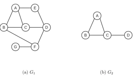
Figure 2 gives a simple example showing a graph G₁ (Figure 2(a)) and one of its subgraphs G₂ (Figure 2(b)). If graph G₂ is used as a subgraph query and graph G₁

is a graph in the database being queried, then G₁ should be returned as one of the query results.

(a)G₁ (b)G₂

Figure 2: An example of a graph and its subgraph

2.2.2 Graph Isomorphism and Subgraph Isomorphism

Two graphs, G₁ and G₂, are the same if it is possible to redraw one of them, say

G₂, so it appears identical to G₁. In graph theory, the term isomorphic is used to describe graphs that are the same but are models of diﬀerent situations. If two graphs

G₁ and G₂ are equivalent graphs, they are referred as isomorphic graphs [Cha85]. The process of graph matching is to determine whether two graphs are isomorphic or not. For instance, the graph G₁ and G₂ in Figure 3 (extracted from [Cha85]) are isomorphic. If two graphs G₁ and G₂ are isomorphic, we say G₁ is isomorphic to G₂

and that G₂ is isomorphic to G₁.

Attributes of vertices are denoted by attr v . The deﬁnition for Graph Map-ping, Graph Isomorphism and Isomorphic Graphs are given below [HS06]

(18)

(a) G₁ (b)G₂

Figure 3: Two isomorphic graphs

[Cha85]:

Deﬁnition 2 Graph Mapping

A mapping between two graphs G₁ and G₂ is a bijection φ : G₁ G₂, where (i) v V₁, φ v V₂, and (ii) e v₁, v₂ E₁, φ e

φ v₁ , φ v₂ E₂.

Deﬁnition 3 Graph Isomorphism and Isomorphic Graphs

A graph isomorphism from G₁ to G₂ is a graph mapping φ from G₁ to

G₂ such that (i) v V₁, φ v V₂ and attr v attr φ v and (ii)

e E₁, φ e E₂ and attr e attr φ e . Two graphs G₁ and G₂ are isomorphic if a graph isomorphism exists from G₁ to G₂. Graph isomor-phism is symmetric.

Given the deﬁnition of isomorphic graphs, the deﬁnition of Subgraph Isomor-phic and Subgraph Isomorphism can then be given as follows.

Deﬁnition 4 Subgraph Isomorphic and Subgraph Isomorphism

A graphG₁is subgraph isomorphic to another graphG₂ifG₁is isomorphic to a subgraph of G₂. A subgraph isomorphism exists between G₁ and

G₂ if G₁ is subgraph isomorphic to G₂. Subgraph isomorphism is not symmetric.

(19)

The subgraph isomorphism problem has long been proved to be NP-complete using a reduction from 3-SAT involving cliques [Coo71]. There has been a lot of research into ﬁnding a fast algorithm for subgraph isomorphism decision. Early research in [Ull76] proposed exact subgraph isomorphism algorithms which are devised for both graph isomorphism and subgraph isomorphism and are still some of the most commonly used algorithms for exact graph matching today. (The subgraph isomorphism algorithm described in [Ull76] is used in this thesis.) [Epp95] proposed a linear time method to solve the subgraph isomorphism problem in planar graphs for any pattern of constant size. [CFSV04] demonstrated an algorithm, namely VF2, for isomorphism problems when matching large graphs. A state-of-the-art subgraph isomorphism algorithm called QuickSI is introduced in [SZLY08].

Having the deﬁnition of subgraph isomorphism, when referred to a subgraph of a graph, we can simply say: a graphG V, E is a subgraph of another graphG V , E

if G is subgraph isomorphic to G under graph mapping φ.

In this thesis, SubgraphIsomorphism G₁, G₂ is used to refer to the subgraph isomorphism test to determine whether or not a graph G₁ is a subgraph of another graph G₂.

2.3 The Filtering-and-Veriﬁcation Framework

Though much research has been done into accelerating the process of subgraph iso-morphism test, the time cost for this process is still heavy. Thus, a direct comparison of a query graph to each of the graphs in the dataset using a subgraph isomorphism algorithm is very ineﬃcient. Diﬀerent graph indexes for graph databases are used to decrease the number of subgraph isomorphism tests for graph queries and therefore gain a better performance in terms of time cost.

Most graph database indexes follow a common framework called Filtering-and-Veriﬁcation [ZCZ 08], as shown in Figure 4.

The filtering step firstly builds an index using the graphs in the dataset. Then the index is used to eliminate some false results (usually most of the false results) and produces a candidate set. The last step is to use the expensive subgraph isomorphism test to verify the candidate set and obtain the final result set [CKNL07]. Since the candidate set is much smaller than the original dataset, it is more efficient to use an

(20)

Figure 4: The filtering-and-verification framework as a pipe and filter system

index than naive sequential scan.

There has been a lot of research about graph indexes using the filtering-and-verification framework. [HLPY10] categorized them into two main types depending on whether they use frequent graph mining. A frequent graph mining algorithm is an algorithm that discovers all subgraphs which occur frequently in the database, with the motivation that these are the subgraphs with a statistically significant amount of occurrences in the database [NK04].

Mining Based Approaches is the first category. The main process of building the index in this category is to extract subgraphs as features in order to obtain a set of feature graphs. Each feature graph is associated with a list of graph IDs which contain this feature graph as a subgraph. In the query process, the candidate graphs are obtained by finding features associated with the posting lists and intersecting the lists. A subgraph isomorphism test is used to refine the candidates to get the final result [HLPY10].

Non-Mining Based Approaches is the second category. Graph indexing and query processing methods in this category do not share the same features. Graph-Grep [SWG02], Summarization graph [ZCZ 08] and Closure-Tree [HS06] are in this category. We will introduce the Closure-Tree in Section 2.5 which forms a basis for our work.

(21)

2.3.1 The False-Positive Rate in Candidate Answer Set

In the ﬁltering phase, the false-positive rate is the probability of categorizing a nega-tive result into the candidate set. Statistically, assumeSC is the candidate answer set

for a query Q after ﬁltering, the result set SR is obtained after verifying Qwith SC,

we have the false-positive rate FP = SC SR

SC . In contrast, the true-positive rate TP

= SR

SC . The false-positive rate can be reduced by selecting some proper ﬁltering

meth-ods, thus to reduce the size of the candidate answer set to speed up the veriﬁcation process.

2.4 Dead Space in Graph Merging

Graph merging is an operation for a set of graphs, sayS, to merge them into a single graphGM erge, in a way that all the graphs inS are subgraphs of the generated graph

GM erge: g S, g is subgraph-isomorphic to GM erge.

Graph merging has an obvious feature for subgraph mining: if a query graph GQ

is a subgraph of one of the graphs in the set S, say G₁, then GQ is a subgraph of

the merged graph GM erge. This is equal saying that, if GQ is not a subgraph of the

merged graph GM erge, then GQ is not a subgraph of any of the graphs in the set S.

This kind of organization of graphs beneﬁts the subgraph mining process because if

GQ is not a subgraph ofGM erge, then no further test is needed to examine each of the

graphs in S, and thus the execution times of the expensive subgraph-isomorphism test is reduced to 1 from up to S.

To use the beneﬁts of graph merging there is a price to be paid in terms ofDead Space. The dead space of a merged graph Gmerge is the space inside Gmerge but

contains no graphs that are in the graph set S [HLPY10]. We use an example in Figure 5 to explain the concept of dead space. Gmergecan be obtained by mergingG1

(Figure 5(a)) and G₂ (Figure 5(b)). It is obvious that Gmerge satisﬁes the condition

that bothG₁andG₂are its subgraphs. There are two simple query graphsGQ1(Figure

5(d)) and GQ2(Figure 5(e)), both of which are not subgraphs of any of the graphs in

S. Table 1 shows a comparison of numbers of subgraph isomorphism tests executed using G₁ and G₂ as query graphs in diﬀerent graph matching strategies.

(22)

(a)G₁ (b)G₂ (c)Gmerge

(d)GQ1 (e)GQ2

Figure 5: An example showing the dead space

of subgraph-isomorphism test is even larger than naive sequential scan of the dataset. Because GQ2 is a subgraph of Gmerge but is not a subgraph of G1 or G2, thus we

considerGQ2 to be a graph in the dead space of Gmerge. There are many more sample

graphs that are in the dead space of Gmerge which make the merged graph somehow

ineﬃcient. The larger the dead space ofGmergeis, the less graph matching can beneﬁt

from graph merging.

The solution to reducing the dead space is to merge only the graphs that are similar in terms of vertices, edges and the structures. The deﬁnition for the term

Query Graph Naive Sequential Scan Graph Merging Pre-process

GQ1 2 1

GQ2 2 3

(23)

Graph Similarity as well as related calculation methods are given in [He07].

2.5 Closure-Tree Index

In this section, we introduce the previous work in [HS06].

2.5.1 Graph Representation

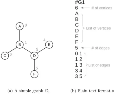
The Closure-Tree (CTree) index is a graph database index for a large number of small graphs which adopts a plain text format for representations of both data graphs and query graphs. Figure 6(a) shows a simple graphG₁ that contains six vertices and ﬁve edges. Figure 6(b) shows the plain text format representation of graph G₁.

(a) A simple graphG₁ (b) Plain text format ofG₁

Figure 6: The graph data and query format in CTree

Each graph entry starts with a ‘#’, and is followed by the components: graph name, number of vertices, list of vertex labels, number of edges, list of edges. The vertices are numbered starting from 0 in the internal representation, which correspond to the numbers in the edge list. The labels of the vertices are limited to alphabetic letters. In the edge list, the order of the two numbers appearing in a line shows the

(24)

direction of an edge. However, throughout the thesis, we use only undirected graphs for both data and query graphs, thus each line in the edge list is recognized as an undirected edge.

An undirected graphG is denoted asG V, E , where V is the vertex set and E is the edge set.

2.5.2 The Graph-Closure Method

In the CTree index, every tree node is a graph or a special kind of graph which is called a graph-closure. Every CTree node contains structural information of all its descendants. Graph-Closure is introduced to capture the structural features of a set of graphs or graph-closures. [HS06] gives the concepts of vertex-closure, edge-closure and a new deﬁnition of graph mapping below:

Deﬁnition 5 Vertex Closure and Edge Closure

The closure of a set of vertices is a generalized vertex whose attribute is the union of the attribute values of the vertices. Likewise, the closure of a set of edges is a generalized edge whose attribute is the union of the attribute values of the edges.

To ensure each vertex and edge have a corresponding element in the mapped graph, dummy vertices/edges are introduced and have a special label ε as their attribute.

Deﬁnition 6 Graph Mapping

A mapping between two graphs G₁ and G₂ is a bijection φ : G₁ G₂, where (i) v V₁,φ v V₂, and at least one ofv and φ v is not dummy, and (ii) e v₁, v₂ E₁, φ e φ v₁ , φ v₂ E₂, and at least one of

e and φ e is not dummy.

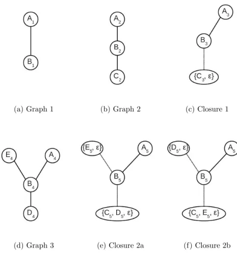
Figure 7 demonstrates an example of constructing a simple CTree. The subscript of each label is used to diﬀerentiate vertices in diﬀerent graphs.

Firstly, Closure 1 is computed from Graph 1 and Graph 2. Note that vertex A, vertex B and edge A, B are common structures between these two graphs. Vertex

C and edge B, C in Graph 2 are not common structures. Vertex C is mapped to a dummy vertex ε and put into a vertex closure C, ε . Edge B, C is mapped to

(25)

(a) Graph 1 (b) Graph 2 (c) Closure 1

(d) Graph 3 (e) Closure 2a (f) Closure 2b

Figure 7: Computing a graph-clousre

a dummy edge ε and put into an edge closure B, C , ε . A dotted line implies an edge-closure. Dummy vertices are used so that every vertex has a corresponding element in the other graph.

Next, in Figure 7(e), Closure 2a is computed from Closure 1 and Graph 3 using the same method. Here the concept of a graph-closure under mappingφ is introduced [HS06].

Deﬁnition 7 Graph Closure under Mapping φ

The closure of two graphs G₁ and G₂ under a mapping φ is a generalized graph V, E where V is the set of vertex closures of the corresponding vertices andE is the set of edge closures of the corresponding edges. This

(26)

is denoted byclosure G₁, G₂ .

In Figure 7(d), vertex E₄ is mapped to ε, vertex D₄ is mapped to C, ε in (c). If D₄ is mapped to ε, then the ﬁnal constructed graph-closure will be (f). [HS06] developed a graph mapping method calledN eighbor Biased M apping (NBM) which maximizes the common structures between two graphs. After NBM, the obtained mapping can be used to merge two graphs, say G₁ and G₂, into a new generalized graph G₃. The process is denoted asG₃ Closure G₁, G₂ .

In the plain text representation format, a graph-closure always has an ID null. A vertex-closure or an edge-closure hasnull following the vertex label or edge numbers indicating that it is a closure. Following the edge list, a graph-closure further has one line indicating how many entries of graphs/graph-closures it has.

2.5.3 Building the CTree and Querying

The graph-closures for a graph dataset are computed recursively level by level. The graph-closure on the top level contains the structural information of all the graphs in the dataset and is the root of this CTree. The constructed tree structure is called a

Closure-Tree (CTree). The CTree building algorithm is shown in Algorithm 1 [HS06].

(27)

Algorithm 1: BuildCTree(S, M)

input : A set of graphs S, the maximum number of entries for each graph-closure M

output: A CTree tree

ClosureSet P artition S ;

if ClosureSet 1 then

tree.Root ClosureSet 1

else

tree.Root M akeClosure ClosureSet ;

return ctree;

FunctionPartition(S)

input : A set of graphs S

output : A set of graph-closures C

if S M then return M akeClosure S ; else S₁ S i i 1, S₂ ; S₂ S i i S₂ 1, S ; C₁ partition S₁ ; C₂ partition S₂ ; if C₁ C₂ M then return C₁ C₂ ; else C₁ M akeClosure C₁ ; C₂ M akeClosure C₂ ; return C₁ C₂; FunctionMakeClosure(C)

input : A set of graphs C

output : A graph-closure G if C 1 then G C 1 ; return G; else G C 1 ; for i 2 to C do G Closure G, C i ; return G;

(28)

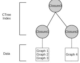
Figure 8 shows a CTree computed from the graphs in Figure 7. Closure3 is the root of this CTree which has a depth of 2. Each graph-closure is a node in the CTree, and each leaf CTree node (Closure1, Closure2) contains graph entries only, while each non-leaf CTree node (Closure3) only contains CTreeNode entries. In order to maintain that only leaf CTreeNodes contain graph entries, Graph4 is ﬁrstly transformed into a graph-closure and then participates in further computing.

In order to distinguish the use of ‘vertex’ and ‘node’, the term ‘node’ is used when we refer to the tree index, The word ‘vertex’ is used when we refer to the graphs in a dataset.

In the graph query process, if a CTree node fails a sub-graph isomorphism test with the query graph, then no children nodes need to be further tested, and thus this node and all its descendants are pruned. If the pruning happens at a relatively higher level of the index tree, then more descendant nodes are likely to be pruned and therefore reduce the query time signiﬁcantly. CTree uses a P seudo Subgraph Isomorphism

test to prune unwanted nodes and uses the subgraph isomorphism test of [Ull76] to further ﬁlter the candidate graph list. The query graphs have the same structure and format as the data graphs. The query process is shown in Algorithm 2 from [HS06].

2.5.4 Histogram-Based Pruning in CTree

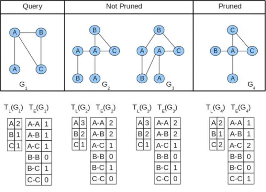
In CTree, a histogram-based method is used as a simple pruning before the structural pruningPseudo-Subgraph Isomorphismtest [HS06]. The pruning starts by calculating the histogram-feature of each graph in the dataset. Assume a query graph G₁ and a data graph G₂ need to be tested. The pruning proceeds in the following steps:

1. Record the number of appearance of each diﬀerent vertex labels in an array TL to get TL G1 and TL G2 . Also record the number of

appearance of edges in an arrayTE to getTE G1 and TE G2 . Note

that TL G1 TL G2 TL, and TE G1 TE G2 TE .

2. if i 1, TL G1 , such thatTL G1 i TL G2 i , prune G2.

3. if i 1, TE G1 , such that TE G1 i TE G2 i , prune G2.

This pruning can also be applied to prune graph-closures because a graph-closure is a generalized graph.

(29)

Algorithm 2: QueryCTree(query, tree)

input : A query graph query, a CTreetree

output: A set of graphs that contain query as a subgraph

CS V isit(query, tree.Root) ;

Ans empty ;

foreach G CS do if SubIsomorphic(query, G) then

Ans Ans G ;

return Ans;

FunctionVisit(query, node)

input : A query graph query, a CTree node node

output : A graph set CS CS empty;

foreach child c of node do

G the graph or graph closure at c;

if PseudoSubIsomorphic(query,G) then if G is a database graph then

CS CS G ;

else

CS CS V isit(query,c);

(30)

A pruning example is shown in Figure 9. G₂ and G₃ both survived the pruning with G₁ as a query graph. But G₁ is not a subgraph of G₃ and G₃ is not pruned, which means the pruning is conservative. G₄ is pruned because TE G4 does not

satisfy the requirements.

Figure 9: The label pruning in CTree

2.6 Regular Expressions

A regular expression is the term used to describe a codiﬁed method that provides a concise and ﬂexible means for matching strings of text [ZYT]. It is usually used to give a concise description of a set of strings without having to list all elements. The IEEE POSIX [IEE] released the Basic Regular Expressions (BREs) along with an alternative standard called Extended Regular Expressions (EREs). BREs provided a common standard which is adopted as the default syntax of many Unix regular expression tools. Most of such tools also provide additional features.

(31)

The GNU C Library [GNU] provides regular expression tools which follow the POSIX.2 standard with support of EREs. We adopt this tool and use EREs in Section 4.1. Detailed introduction of regular expressions can be found in [Goo05] and [Fri97].

(32)

Chapter 3 ECTree: the Extended

Closure-Tree for Subgraph Queries

Using a tree structure in a graph database index allows eﬃcient subgraph structure mining. Section 2.5 introduced Closure-Tree (CTree) which adopts a tree structure in substructure graph mining. However, considering that the labels may not be the only attribute that a vertex can have, CTree is not able to index vertices with additional attributes other than vertex labels.

We adopt the CTree index structure to capture common structures in graphs and focus on subgraph queries, meanwhile, we extend it with additional integer attributes on the vertices.

This chapter is organized as follows: Section 3.1 presents our extensions on the vertex attributes. Section 3.2 discusses the vertex merging methods after the exten-sions. Section 3.3 shows the building process of the ECTree. Section 3.4 gives a query format for the ECTree. Section 3.5 discusses the matching between a query graph and a data graph.

3.1 Extending the Vertices with Attributes

The existing CTree provides access to subgraph mining focusing on vertex labels and edge relations. However, actual graphs could contain more information on the vertices than only the labels. For example, chemical compounds, social networks, etc. have additional information of diﬀerent types on each vertex. In this section, we ﬁrstly

(33)

demonstrate an example of a chemical structure that has both label attributes and numerical attributes. Then we show our method to represent it as a graph in plain text format.

3.1.1 An Example in the SDF Format

SDFstands for structural-data file. It is one of a family of chemical-data file formats developed by MDL [DNH 92]. The SDF format is a text-based format for representing chemical compounds, in which the structural information and associated data items for one or more compounds are contained. An SDF format chemical consists of some header information, a connection table containing the atom info, the bond connections and types, followed by some sections of more complex information. The file format can be V2000, V3000 or a combination of both [Sym].

(a) ISIS/Draw version of Alanine

(b) Connection table of Alanine [Sym]

Figure 10: Alanine in SDF format

Figure 10(a) shows a chemical compound Alanine[NC05] drawn from a chemical structure drawing program called ISIS/Draw [LWSO04]. Figure 10(b) shows the connection table (CTab) of Alanine.

The first line is the counts line which specifies the number of atoms, bonds, and atom lists, the chiral flag setting, and the CTab version. Line 2-7 shows the atom

(34)

block which specifies the atomic symbol and any mass difference, charge, stereochem-istry and associated hydrogens for each atom. Line 8-12 shows the bond block which specifies the two atoms connected by the bond, the bond type and any bond stereo-chemistry and topology (chain or ring properties) for each bond. The last 3 lines are the property block that is provided for future expandability of CTab features, while maintaining compatibility with earlier CTab configurations. Detailed meaning of the values of the atom properties can be found in Appendix A.

We adopt the atom names as vertex labels, the property lists as vertex attributes and the bonds as edges in our ECTree index.

3.1.2 Data Representation in ECTree

We begin by transformingAlanine into the graph shown in Figure 11(a). Besides the vertex label, each vertex further has three more integer attributes adopted from 10(b). In order to store these additional attributes in text format, three positions after each vertex label are added, separated by a “ ”, shown in Figure 11(b). The numbers of integer attributes on each vertex are the same and can be deﬁned according to actual use of the dataset.

Here we give the deﬁnitions of data attribute vector, data vertex and data graph:

Deﬁnition 8 Data Attribute Vector, Data Vertex and Data Graph

A data attribute vector is a vector that contains only integers as its ele-ments. A data vertex is a vertex that has a data attribute vector as its attribute vector. A data graph is a graph that contains only data vertices. The data attribute vector Λv of a data vertexv is formally deﬁned here:

Λv a1, a2, ..., an , ai Z, i 1, n (1)

Each element ai of Λv is an attribute value of the data vertex v. All the graphs

from a dataset are always used as data graphs. Since a graph-closure is treated as a generalized graph, all graph-closures are data graphs.

There are some reasons that we deﬁne the data attribute vector to contain only integer numbers but not other data types such as string or boolean. Firstly, if the attribute contains strings, then the strings have to be matched exactly in the vertex

(35)

(a) The graph format ofAlanine (b) Text representation of (a)

Figure 11: Data structure of ECTree

mapping phase, which is not any diﬀerent than having an extra label. Secondly, a pruning method can be developed with the numbers as attributes, this is discussed later in Section 4.2. Thirdly, in the validation chapter (Chapter 5), the datasets use only integers as attributes of the vertices. Besides, it is very simple to extend the attributes to real numbers if there is need.

3.2 Vertex Merging

The vertex matching phase in building a CTree is very simple: to check whether two vertices have the same label or not, if they do, then the two vertices match, otherwise they do not match. We deﬁne the label-matching for two data vertices in ECTree as follows: two data vertices label-match if these two data vertices have the same label. Now we consider the attribute vector of a vertex. In CTree, if two vertices are label-matched, there is no additional operations for merging them. In ECTree, we need to modify the vertex merging strategy so that the label-matched vertices or the non-label-matched vertices which are made into a vertex closure still capture necessary information for the later querying phase. CTree uses each graph-closure as

(36)

a “bounding box” of constituent graphs which contains discriminative information of their descendants [ZYY07]. We want our index to inherit the feature of “bounding box” on the attributes as well, thus the merging methods of vertex/vertex-closures are taken into account.

There are three diﬀerent cases to discuss in the vertex merging phase: i) merg-ing two vertices, ii) merging a vertex and a vertex-closure, iii) merging two vertex-closures. We ﬁrstly ignore the integer attributes and map two graphs using Neighbor Biased Mapping, then we consider each of the merging cases separately in detail. In this section, we only discuss the merging methods, the graph mapping method

Neighbor Biased Mapping is adopted from [HS06].

3.2.1 Merging Two Vertices

The main purpose of the closure-tree structure is to reuse common sub-structures. Therefore the merging of two or multiple vertices is a very frequent operation. Merging multiple vertices can be composed of a series of operations of merging two vertices, so we only discuss binary operations here.

Figure 12 shows two vertices va and vb that have the same label. The merged

vertex from two label-matched vertices is a vertex with the same label. va andvb are

merged intovmergedshown in Figure 12(c). For each attributeai invmerge, we set it to

the maximum absolute value at the same position of the merging vertices. Λvmerged 1

= M ax Λva 1 , Λvb 1 =M ax 5, 3 = 5.

(a)va (b)vb (c)vmerged Figure 12: Merging two label-matched vertices

If a vector Λv needs to be merged from multiple vectors Λv₁, ...,Λv_M, M 1, we

(37)

Equation 2: (Note that when the notation A is used, if A is a set, then A is the cardinality of A; if A is a number, then A is the absolute value ofA.)

M erge Λv₁, ...,ΛvM M ax Λvi 1 i 1, M , ..., M ax Λvi n i 1, M (2)

Since the attribute vector of the merged vertex is the absolute ceiling of the all merging vertices, we denote it by a comparison operator “ ”: Λvmerged Λvi,

i 1, M . The deﬁnition for the operator “ ” between two data attribute vectors are given in Equation 3. (Note that we have Λva Λvb Λ )

Λva Λvb Λva i Λvb i , i 1, Λ (3)

According to Equation 2 and 3, it can be inferred that:

M erge Λv₁, ...,ΛvM Λvi, i 1, M (4)

Next we take a look at the merging of two non-label-matched vertices. The merged vertex from two non-label-matched vertices is a vertex-closure which has a list of attribute vectors of each of the vertex included in the merging. The structure of a vertex-closure in ECTree index has two parts: a label set and an attribute vector list. We further discuss two subcases in vertex merging.

The ﬁrst subcase is that a vertex v is mapped to a dummy vertex vε. Figure

13(a)(b)(c) shows that a vertex va is mapped to a dummy vertex vε and they are

both added to a vertex-closure vmerged. A dummy vertex in ECTree has the same

label as in CTree: ‘ε’, and has an empty attribute vector Λ . When a vertex v is added to a vertex-closure vmerged, the label of v is added to the label set of vmerged,

each attribute in the vertex attribute vector ofv is transformed into the corresponding absolute value, and then the attribute vector is added to the attribute vector list of

vmerged. If the vertex to be added is a dummy vertex, the label ‘ε’ is added to the

label set of vmerged and Λ is added to the attribute vector list of vmerged.

The second subcase is that a vertex v₁ is mapped to another vertex v₂ which has a diﬀerent label. Both labels of v₁ and v₂ are added to the label set of vmerged, and

all attributes of vectors of v₁ and v₂ are transformed into the corresponding absolute value and added to the attribute vector list of vmerged. Figure 13(d)(e)(f) shows an

(38)

Assume the number of distinctive labels in a graph database is D, the upper bound for the size of a vertex-closure in the ECTree index is D 1 because of a possible dummy vertex.

(a)va (b)vε (c)vmerged

(d)vb (e)vc (f) vmerged Figure 13: Merging two non-label-matched vertex

3.2.2 Merging A Vertex and A Vertex-Closure

In this case, we merge a vertex v and a vertex-closure vc into a new vertex-closure.

There are two possible subcases: 1) the vertex-closurevclosure contains a vertex label

that is the same as the label of v, 2) the vertex-closure vclosure does not contain any

vertex label that is the same as the label of v.

In subcase 1), the merging vertex v has a same label l (l ‘B’ in Figure 14(a)) of one of the labels in the vertex-closure vclosure, we update the vertex attribute

vector Λl in the vertex-closure using the attribute vector Λv according to Equation

2: Λl new M erge Λl,Λv . If the label of the merging vertexv is ε, then the merged

vertex-closurevmerged is the same as the merging vertex-closure vclosure, no operations

are needed. An example of the merging is shown in Figure 14(a)(b)(c).

In subcase 2), the process is similar to merging two unmatched vertices but to replace one vertex by a vertex-closure in this case. An example is shown in Figure

(39)

(a)va (b)vclosure (c)vmerged

(d)va (e)vclosure (f) vmerged Figure 14: Merging a vertex and a vertex-closure

14(d)(e)(f).

3.2.3 Merging Two Vertex-Closures

In this case, two vertex-closures vclosure1 and vclosure2 are merged into a new

vertex-closure vmerged. We still have two possible subcases: 1) the two vertex-closure label

sets do not have any vertex labels in common, 2) the two vertex-closure label sets have some vertex labels in common. The ﬁrst subcase is similar to merging two unmatched vertices, we simply add the labels and corresponding attribute vectors into a new vertex-closure, no further operations are needed. We mainly discuss the two steps in merging two vertex-closures that have same labels. Assume L₁ is the label set of vclosure1, L2 is the label set of vclosure2.

Step 1:

if the common label l ‘ε’: add l to the label set of vmerge, add Λl new

M erge Λl₁,Λl₂ to the attribute vector list, l1 l2 L1 L2, l1 L1,l2 L2.

if the common label l ‘ε’: add ε to the label set of vmerge, add Λ to the

(40)

Step 2, l L₁ L₂ L₁ L₂ , add l to the label set of vmerge and add Λl to the

attribute vector list.

(a)vclosure1 (b)vclosure2 (c)vmerged Figure 15: Merging two vertex-closures

An example of this case is shown in 15, vclosure1 and vclosure2 have two labels in

common: l₁ = ‘B’ and l₂ = ‘C’, while ‘ε’ and ‘D’ are not common labels. Thus we use Equation 2 to calculate the new attribute vector in vmerge: Λmerged l₁ =

M erge Λclosure1 l₁,Λclosure2 l₁ , Λmerged l₂ = M erge Λclosure1 l₂,Λclosure2 l₂ . ‘ε’ and

‘D’ are directly added to the list of attribute vectors without any operations.

3.3 Building the ECTree

We modified the data representation of a graph in the dataset, thus the structure of a graph-closure and its computing method have to be modified accordingly. Since the structure of edges and edge closures are not modified, the corresponding methods do not need modifications. We focus on our new methods of computing graph closures in this section.

3.3.1 Data Graph Mapping

In CTree, there is no distinguishment between mapping two data graphs and mapping a query graph and a datagraph. We will introduce the mapping between a query graph and a data graph for ECTree in Section 3.4.

(41)

In order to make two graphs G₁ and G₂ into a graph-closure C, it is necessary to ﬁnd a possible graph mapping φ initially from G₁ to G₂. In ECTree, we get the graph mapping φ by using Neighbor Biased Mapping, ignoring the attributes of the vertices; then each mapped pair of vertices/vertex-closures are merged using previous described methods.

We do not do exact matching for data graph mapping for the following reasons. Firstly, the possibility for two vertices in two graphs to have the exact same label and attributes is very low; secondly, we still maintain the clustering feature of the tree index using the vertex merging methods.

3.3.2 An ECTree Building Example

The process of building graph-closures is the process of building an ECTree. We show an example of building a graph-closure from three graphs in a dataset in Figure 16.

Firstly Closure 1 is computed from Graph 1 and Graph 2. For vertex C in Graph 2, there is no corresponding vertex so it is mapped to a dummy vertex ε, both of them are put into a vertex-closure C, ε .

Next we compute Closure 2a from Closure 1 and Graph 3 using the same method, as shown in Figure 16(e). Figure 16(f) shows Closure 2b which is computed from Closure 1 and Graph 3 as well but using a different graph mapping. Graph mappings can be obtained using different graph mapping algorithms, but for a chosen algorithm, the mapping obtained between two graphs is unique. Ideally, the mapping method should maximize the common structure and attributes of the two graphs. Since we did not find a proper mapping algorithm for attributed graphs, the NBM [HS06] method is used.

3.4 A Query Graph Format for ECTree

Just like CTree, we can also use a data graph as a query graph. For instance, to query the substructure as shown in Figure 11(a), the representation in Figure 11(b) can simply be used as a query. However, in ECTree, we focus on the graph data mining of the attributes of the vertices, the use of the format of the data graphs as query graphs is too simple and does not make full use of the new index. We introduce

(42)

(a) Graph 1 (b) Graph 2 (c) Closure 1

(d) Graph 3 (e) Closure 2a (f) Closure 2b

Figure 16: Computing a graph-closure in ECTree

a query format for ECTree that allows more ﬂexible queries in terms of the attributes of vertices.

Firstly, we allow the use of intervals to appear in the query graphs. An integer interval is made up of two integers and two brackets. An open or close bracket means the integer at that side is not included in the interval, while a square bracket means the integer at that side is included in the interval.

Two or more intervals can be used together to make up more complex intervals. Some examples of interval sets are shown in Figure 17(a): I₁ 0,1 , I₂ 4, 2 ,

I₃ 1,2 2,3 4,5 , I₄ 9. There is only one relational operator “ ” union supported between the intervals. Since there is only one relational operator, we omit

(43)

it in the representation and by default, it is implied that the union operation is used between all the intervals using together.

(a) Four intervals (b) A graph with intervals

Figure 17: Examples of interval sets

Therefore, [-2,2] (5,7] is written as [-2,2](5,7] in plain text format. I₃ is written as

I₃ 1,2 2,3 4,5 . I₄ can both be written as 9 orI₄ 9,9 . But if a single integer valuei is unioned with other intervals, it has to be written in the form of i, i . E.g, 5 [6.8] should be written as [5,5][6,8]. Figure 17(b) shows a query graph Q which uses the intervals in the graph attribute vectors.

In addition to the integer intervals described above, we use the symbol ‘*’ to replace the interval , . The symbol ‘*’ cannot be unioned with any other interval(s). E.g., the plain text format of the query vertex ‘D , [-2,-2]’ is written as ‘D [-2,-2]’.

In contrast to Deﬁnition 8, we give the deﬁnitions for Query Attribute Vector, Query Vertex and Query Graph here:

Deﬁnition 9 Query Attribute Vector, Query Vertex and Query Graph

A query attribute vector is a vector that contains integer interval sets as its elements. A query vertex is a vertex that has a query attribute vector

(44)

as its attribute vector. A query graph is a graph that contains query vertices.

Let Ii, i 1, n be a set of integer intervals, we denote the query attribute vector

Λ_v as follows:

Λv I1, I2, ..., In (5)

3.5 Query Matching

In this section, we discuss the query matching for ECTree graph index. We have demonstrated diﬀerent formats of the query graphs and the data graphs as well as the methods to make the graph-closures in ECTree. There are two diﬀerent cases in the query matching: matching a query with a non-closure graph and a graph-closure. In both cases, we assume the mapping φ between a query graph and a data graph is obtained by using the graph mapping algorithm Neighbor Biased Mapping from [HS06].

3.5.1 Matching a Query Vertex and a Data Vertex

There are two cases to discuss: 1) matching a query vertex and a data vertex in a non-closure graph, 2) matching a query vertex and a data vertex in a graph-closure. In the ﬁrst case, a query vertexvQmatches a data vertexvD in a non-closure graph

if Λv_D i ΛvQ i , i 1, ΛvQ . This is easy to understand because a non-closure

data vertex is in the vertex set of a non-closure graph which is in the original dataset. An example is shown in Figure 18. vQ matches vD1 but does not match vD2.

(a)vQ (b)vD₁ (c)vD₂

Figure 18: Matching a query vertex and a non-closure data vertex

For simpliﬁcation, we deﬁne the operator “ ” between a query attribute vector and a data attribute vector of a non-closure vertex in Equation 6:

(45)

Λ Λ Λ i Λ i , i 1, Λ (6) In the second case, since the attribute vector of a vertex-closure is the absolute ceiling of all the attribute vectors in the closure, we only compare the values in the data attribute vector to the minimum absolute values of the intervals in the query vector. We denote the minimum absolute value within a interval set I by Min-Absolute(I) = M in i i I . E.g., in Figure 19(a) Min-Absolute(I) = i₂, in Figure 19(b) Min-Absolute(I) = 0. Here the deﬁnition of the operator “ ” between a query attribute vector and a data attribute vector of a graph-closure is given in Equation 7.

Λ Λ Λ i Min-Absolute Λ i , i 1, Λ (7)

We take a look at the two examples in Figure 19. Assume I i₁, i₂ i₃, is an interval set in a query attribute vector Λ I , i₁ i₂ i₃, i₂ i₃. d₁ 0, d₂

0, d₂ d₁ are two values in two diﬀerent data attribute vector Λ₁ = d₁ and Λ₂ d₂ . In Figure 19(a), the query interval requires the value of the data attribute falls in the interval set I, but for Λ₁, the value can only fall within d₁, d₁ which means all the values of the attribute of the vertices in the vertex-closure are within d₁, d₁

thus cannot match I. In this case, only Λ₂ satisﬁes the condition. In Figure 19(b), the value ‘0’ is included in the interval set I, therefore the minimum absolute value within I is ‘0’. Sinced₁ 0 and d₂ 0, they both satisfy the condition.

(a) (b)

(46)

We sum the matching between a query attribute vector Λ_v

Q and a data attribute

vector ΛvD as follows:

Λ Λ Λ i Λ i , i 1, Λ vQisnon-closure Λ i Min-Absolute Λ i , i 1, Λ vQis a closure

The modiﬁed vertex mapping algorithm is shown in Algorithm 3.

Algorithm 3: VertexMapping Modiﬁed(v₁, v₂)

input : A query vertex v₁, a data vertexv₂

output: A boolean value, trueif mappable, false if not

if label of v₁ does not match label of v₂ then return false;

Λ attribute vector of v₁ ; Λ attribute vector of v₂ ;

if v₂is from a graph-closure then for i 1 to Λ do k Min-Absolute Λ i ; if Λ i k then return false ; else for i 1 to Λ do booleanb false; interval set I Λ i ; for j 1 to I do if Λ i I j then b true; break; if b is false then return false; return true;

3.5.2 Matching a Query Graph and a Data Graph

Based on our discussion in the previous subsection, we deﬁne the subgraph matching as follows:

(47)

A query graph GQ VQ, EQ matches a data graphGD VD, ED if GQ is

subgraph-isomorphic to GD under graph mappingφ and v VQ,Λv Λφ v .

When a query graph is compared to a data graph, the histogram pruning is used ﬁrstly, followed by the Pseudo Subgraph Isomorphism test, and ﬁnally the subgraph isomorphism test. Assume GQ is a query graph and GD is a data graph, Table 2

shows the descriptions of the symbols to be used.

Symbol Description

n₁ the number of vertices in GQ

n₂ the number of vertices in GD

d₁ the maximum vertex degree inGQ

d₂ the maximum vertex degree inGD

l the pseudo compatibility level deﬁned for the

PSI pruning [HS06]

M the time complexity of maximum cardinality

matching for bipartite graphs

a the number of vertex attributes

Table 2: Notations

The worst case complexity for the histogram pruning in ECTree is the same as CTree: O n2₁ , since all calculations are one-time-cost and pre-processed. The PSI pruning algorithm for ECTree has a worst case complexity of O ln₁n₂ d₁d₂ M d₁, d₂ aM n₁, n₂ [HS06]. The pseudo compatibility level is deﬁned before querying and can be adjusted. Hopcroft and Karp’s algorithm [HK71] ﬁnds a maxi-mum cardinality matching in O n2.5 _time.

Here we do some further discussions aboutExact MatchingandInexact Match-ing. When we match a query vertex vQ and a data vertex vD1 from a non-closure

graph, we use exact matching. That is, the attribute values of ΛD1 need to be

in-cluded in the corresponding intervals of Λ_Q. When we match a query vertex vQ and

a data vertex vD2 from a graph-closure, we use inexact matching which means the

attribute values of ΛD2 do not have to exactly match the corresponding intervals of

Λ_Q, but just be larger than the corresponding absolute minimum values. There are a few reasons why we do not use exact matching:

(48)

graph-closures at each level will cost a huge amount of space and thus make the index very large.

On time consumption, if we store a list for each position in an attribute vector, then matching a query attribute vector and a data attribute vector will be very trivial and the time cost can be unacceptable. At a relatively higher level, the lists in the attribute vectors can be very long and hard to update.

The dead space in graph merging needs to be considered as well. Even if a query graph and a graph-closure are matched using exact matching, there is no guarantee that there are answer graphs under the branch of this graph-closure because the matched graph could be in the dead space.

3.6 Conclusion

In this chapter, we have provided description of our extended closure-tree that man-ages graph data with integer attributes on the vertices, based on the original CTree index. ECTree is a graph index that specifies the queries on the vertex attributes and at the same time provides very flexible formats of queries in terms of the at-tributes. We discussed the new merging and matching methods in ECTree for the new structure of both data and query graphs which is very different from the CTree index.

The ECTree index inherits the feature of CTree: graph clustering hierarchically. An ECTree node is the clustering of both the structure and the attribute of its descendents.

ECTree: An Extended Tree Index Structure for Attributed Subgraph Queries

ECTREE: AN EXTENDED TREE INDEX STRUCTURE

FOR ATTRIBUTED SUBGRAPH QUERIES

Concordia University

School of Graduate Studies

Abstract

ECTree: An Extended Tree Index Structure for Attributed Subgraph

Queries

Dedication

Contents

List of Figures

List of Tables

Chapter 1

Introduction

1.1

Graph Data

1.2

The Problem

1.3

Contributions

1.4

Thesis Organization

Chapter 2

Background

2.1

Graph Databases

2.2

Subgraph Query and Matching

2.2.1

Subgraph and Subgraph Query

2.2.2

Graph Isomorphism and Subgraph Isomorphism

2.3

The Filtering-and-Veriﬁcation Framework

2.3.1

The False-Positive Rate in Candidate Answer Set

2.4

Dead Space in Graph Merging

2.5

Closure-Tree Index

2.5.1

Graph Representation

2.5.2

The Graph-Closure Method

2.5.3

Building the CTree and Querying

2.5.4

Histogram-Based Pruning in CTree

2.6

Regular Expressions

Chapter 3

ECTree: the Extended

Closure-Tree for Subgraph Queries

3.1

Extending the Vertices with Attributes

3.1.1

An Example in the SDF Format

3.1.2

Data Representation in ECTree

3.2

Vertex Merging

3.2.1

Merging Two Vertices

3.2.2

Merging A Vertex and A Vertex-Closure

3.2.3

Merging Two Vertex-Closures

3.3

Building the ECTree

3.3.1

Data Graph Mapping

3.3.2

An ECTree Building Example

3.4

A Query Graph Format for ECTree

3.5

Query Matching

3.5.1

Matching a Query Vertex and a Data Vertex

3.5.2