SECOND-ORDER REFINEMENT OF EMPIRICAL LIKELIHOOD
FOR TESTING OVERIDENTIFYING RESTRICTIONS
By
Yukitoshi Matsushita and Taisuke Otsu
April 2011
Revised January 2012
COWLES FOUNDATION DISCUSSION PAPER NO. 1791
COWLES FOUNDATION FOR RESEARCH IN ECONOMICS
YALE UNIVERSITY
Box 208281
New Haven, Connecticut 06520-8281
Second-order refinement of empirical likelihood for testing
overidentifying restrictions
∗
Yukitoshi Matsushita
†Graduate School of Humanities and Social Science
University of Tsukuba
Taisuke Otsu
‡Cowles Foundation & Department of Economics
Yale University
January 2012
Abstract
This paper studies second-order properties of the empirical likelihood overidentifying restriction test to check the validity of moment condition models. We show that the empirical likelihood test is Bartlett cor-rectable and suggest second-order refinement methods for the test based on the empirical Bartlett correction and adjusted empirical likelihood. Our second-order analysis supplements the one in Chen and Cui (2007) who considered parameter hypothesis testing for overidentified models. In simulation studies we find that the empirical Bartlett correction and adjusted empirical likelihood assisted by bootstrapping provide reasonable improvements for the properties of the null rejection probabilities.
1
Introduction
The generalized method of moments (GMM) by Hansen (1982) has been a standard tool for empirical economic analysis. GMM provides a unified framework for conducting statistical inference when economic models are specified by some moment conditions. However, the literature indicates that there are considerable problems with GMM particularly in its finite sample performance, such as the bias in point estimation and distortions of null rejection probabilities in hypothesis testing (see, e.g., the special issue of the Journal of Business and Economic Statistics, vol. 14).
One well-known problem of GMM-based inference is that the (first-order) asymptotic null distribution of the overidentifying restriction test based on the minimized GMM criterion function, often called the J-test, can be a poor approximation in finite samples. In order to overcome this problem, several alternative inference
∗The authors would like to thank a co-editor, two anonymous referees, and the seminar participants at Hiroshima University and
University of Tokyo and Tsukuba for helpful comments.
†E-mail: [email protected]. Address: 1-1-1, Tennoudai, Tsukuba, Ibaraki 305-8571, Japan. Phone:
+81-29-853-4075.
‡E-mail: [email protected]. Website: http://cowles.econ.yale.edu/faculty/otsu.htm. Address: P.O. Box 208281, New Haven,
methods have been developed. Hall and Horowitz (1996) proposed a uniform weight bootstrap method by using recentered moment restrictions. Brown and Newey (2002) proposed a weighted bootstrap method based on the implied probabilities obtained from the moment conditions. These bootstrap methods provide higher-order refinements for the property of null rejection probabilities of overidentifying restriction tests.
Another approach to tackle this finite sample problem of the GMM-based overidentifying restriction test is to employ an alternative criterion function to derive a test statistic, such as continuous updating GMM, exponential tilting, and empirical likelihood (see, Kitamura, 2007, for a survey). Among them, empirical likelihood is an attractive candidate to deal with the distortion problem of the null rejection probabilities because of its Bartlett correctability, a second-order refinement based on the Edgeworth expansion. The Bartlett correctability of the empirical likelihood-based test is reported in several contexts, such as smooth functions of means (DiCiccio, Hall and Romano, 1991) and quantiles (Chen and Hall, 1993). Also Baggerly (1998) focused on testing for the mean parameter (i.e., E[X] = 0) and showed that only empirical likelihood is Bartlett correctable in the power divergence family. Bravo (2004) showed that a bootstrap version of the empirical likelihood test achieves the same higher order accuracy as the Bartlett corrected test. Although the parameters of interest are different, these papers studied Bartlett correctability of empirical likelihood in just-identified moment restrictions (i.e., the number of moment restrictions equals the number of parameters). This paper is concerned with overidentified moment restrictions (i.e., the number of moment restrictions exceeds the number of parameters) which are common in economic analysis. Although the second-order analysis becomes substantially more complicated due to extra systems and terms brought by overidentifying restrictions, Chen and Cui (2007) tackled this problem and showed that the empirical likelihood test for parameter hypotheses is Bartlett correctable even if the models are overidentified.
This paper extends Chen and Cui’s (2007) analysis to the overidentifying restriction testing problem and studies second-order properties of the empirical likelihood overidentifying restriction test. Although the basic idea of the second-order analysis follows from Chen and Cui (2007), the technical detail is case-by-case and specific to our test statistic. Indeed Chen and Cui (2007, p. 504) indicated the possibility of this extension, and this paper formally studies this issue. In particular, we show that the empirical likelihood test for overidentifying restrictions is also Bartlett correctable and propose second-order refinement methods for the test based on the empirical Bartlett correction and adjusted empirical likelihood. Adjusted empirical likelihood (Liu and Chen, 2010) is a modification of empirical likelihood to avoid non-existence of solutions for the likelihood maximization problem by introducing auxiliary observations. Our refinement methods are illustrated by simulation studies based on a linear instrumental variable regression model and asset pricing model. We find that (i) the GMM and empirical likelihood tests based on the asymptotic critical values show severe over-rejections particularly when the number of moment restrictions is large, and (ii) an empirical Bartlett correction and adjusted empirical likelihood assisted by bootstrapping provide reasonable improvements for the properties of null rejection probabilities. Since testing for overidentifying restrictions is a fundamental problem to assess the validity of economic theory which precedes to parameter estimation and inference, our refinement methods contribute to enhance the reliability of empirical economic analysis based on moment condition models.
In the context of hypothesis testing for overidentifying restrictions, there are several papers which derive global optimal properties of empirical likelihood-based tests. Kitamura (2001) focused on the generalized Neyman-Pearson criterion (i.e., comparison of decay rates of the type II errors under fixed alternatives subject to a restriction on the decay rate of the type I errors), and showed that the empirical likelihood test is generalized Neyman-Pearson optimal. Otsu (2010) focused on the Bahadur criterion (i.e., comparison of decay rates of
p-values under fixed alternatives), and showed that the empirical likelihood test is Bahadur optimal. Canay and Otsu (2011) focused on the Hodges-Lehmann criterion (i.e., comparison of decay rates of the type II errors under fixed alternatives subject to a size constraint), and showed that not only the empirical likelihood test but also the GMM and generalized empirical likelihood tests are Hodges-Lehmann optimal. These studies concentrate on global (or fixed alternative) and first-order power properties and show that the empirical likelihood test satisfies these optimality criteria. On the other hand, this paper concentrates on second-order null rejection properties under the null hypothesis and show that the empirical likelihood test is Bartlett correctable (i.e., accepts a second-order refinement for the null rejection property). If the Bartlett correction factorBc for the empirical likelihood test Tn is known, then the corrected test statistic Tn!
1 +n−1Bc"−1
shows the same first-order global power properties to the original statisticTn. Thus, the Bartlett corrected empirical likelihood test also enjoys the above global optimal properties. However, if Bc is unknown (as always the case in practice) and is estimated byBcˆ based on data, then we need to incorporate the large deviation properties of the estimation errorBcˆ −Bcand the first-order global power properties of the corrected test statisticTn#1 +n−1Bcˆ $−1 require further investigation.
Based on these considerations, we recommend applied researchers to employ the Bartlett corrected empirical likelihood test (with estimatedBc) when from previous studies the distortion in the null rejection probability is a major concern for their applications of interest, and to employ the uncorrected empirical likelihood test when the distortion in the null rejection probability is not a serious problem and better power property is desired. For example, our simulation results in Section 4 indicate that when the sample size is small and/or the number of moment conditions is large, the uncorrected empirical likelihood and GMM-based overidentification tests tend to over-reject the null hypothesis. Therefore, in such situations, we recommend the use of the Bartlett corrected empirical likelihood test suggested in this paper.
The rest of the paper is organized as follows. Section 2 introduces our setup and notation. Section 3 presents the main theoretical results: second-order properties of the empirical likelihood test statistic and refinements by the Bartlett correction and adjusted empirical likelihood. Section 4 conducts simulation studies based on a linear instrumental variable regression model and asset pricing model. Section 5 concludes. All technical details are contained in the Appendix.
2
Setup
Our notation closely follows that of Chen and Cui (2007). Suppose we observe a random sample{Xi}ni=1 from
X ∈X ⊆Rd. Letg :X ×Θ→Rr be a vector of moment functions, whereΘ⊂Rp is the parameter space and r > p(overidentified). We wish to test the validity of the overidentifying restrictions:
H0:E[g(X,θ)] = 0 for someθ∈Θ,
H1:E[g(X,θ)] (= 0 for anyθ∈Θ. (1)
If the null hypothesis is uniquely satisfied at someθ0∈Θ(i.e., the model is correctly specified and the parameter
is point identified at θ0), then we can estimate the true parameter valueθ0 by GMM or generalized empirical
likelihood and also conduct hypothesis testing onθ0 by the Wald, Lagrange multiplier, or likelihood ratio type
tests. In contrast to Chen and Cui (2007) who focused on parameter hypothesis testing (i.e.,HP
0 :θ0=cagainst
HP
1 :θ0 (=c), this paper studies second-order properties of the empirical likelihood test for the overidentifying
restrictionsH0 against H1. We consider the following setup adopted by Chen and Cui (2007). Let g(X,θ) =
!
g1(X,θ), . . . , gr(X,θ)""
Assumption.
1. {Xi}ni=1 is i.i.d.
2. E[g(X,θ)] = 0 is uniquely satisfied at θ0∈Θ, Θis compact, V =V ar(g(X,θ0))is positive definite, and
G=E%∂g(X,θ0)
∂θ!
&
has the full column rank.
3. There exists a neighborhood N of θ0 such that for each j = 1, . . . , r, gj(x,θ) is continuously third-order
differentiable inθ∈N almost surely and the derivatives are bounded by integrable functions over N. 4. E%|g(X,θ0)|15
&
<∞andlim sup|t|→∞|E[exp (it"g(X,θ0))]|<1.
The same comments in Chen and Cui (2007) apply here. Assumption 1 excludes dependent data. An extension to time series data is beyond the scope of this paper. The first condition in Assumption 2 says that the overidentification null hypothesisH0is satisfied and the true parameter valueθ0is point identified. The last
condition in Assumption 2 excludes weak identification (or weak instruments) in the sense of Stock and Wright (2000). If Assumption 2 does not hold andGdrifts to the zero matrix at the√n-rate (so-called weak identification asymptotics), the first-order asymptotic null distribution of the overidentification test statistic typically becomes non-standard. Assumption 3 is on smoothness of the moment functions. This assumption excludes, for example, quantile regression models. Assumption 4 imposes bounded moments and a Cramér condition used to establish the validity of the Edgeworth expansion. It is known that the Cramér condition is satisfied when the distribution of g(X,θ0)has a non-degenerate and absolutely continuous component (see, e.g., Hall, 1992, pp. 65-67). This
requirement is typically satisfied whenX is continuous andg(x,θ0)is smooth inx. For example, Assumption 4
can be verified for the simulation design in Section 4 motivated by an asset pricing model, and linear instrumental variable regression models with normal errors, regressors, and instruments. However, when the distribution of g(X,θ0)has no absolutely continuous component, a conventional argument to verify the Cramér condition is not
applicable in general, and the validity of the Cramér condition becomes questionable or at least hard to verify.1
We now introduce the empirical likelihood test statistic forH0. LetT be anr×rorthogonal matrix satisfying
T V−1/2GU =!
Λ,0p×(r−p)
"" ,
whereU is ap×porthogonal matrix andΛis ap×pnon-singular diagonal matrix. We orthogonalize the moment functions as wi(θ) = T V−1/2g(Xi,θ) so that E'
wi(θ0)wi(θ0)"( =I. The empirical likelihood overidentifying
restriction test statistic, proposed by Qin and Lawless (1994), can be defined as
Tn= min θ∈Θ"(θ) = minθ∈Θ2 n ) i=1 log! 1 +λ(θ)"wi(θ)" , where λ(θ) solves*ni=1 wi(θ)
1+λ!wi(θ) = 0 with respect toλ for a given value of θ. From Qin and Lawless (1994,
Corollary 3), we can see thatTn→d χ2(r
−p)underH0.
The rest of this section presents an expansion formula for Tn derived by Chen and Cui (2007). Let θˆ =
arg minθ∈Θ"(θ)andˆλ=λ
# ˆ
θ$. The first-order conditions for#λˆ",θˆ"$are written asQ#λˆ,θˆ$= 0, where
Q(λ,θ) = + 1 n n ) i=1 wi(θ)" 1 +λ"wi(θ), 1 n n ) i=1 λ"(∂wi(θ)/∂θ") 1 +λ"wi(θ) ," . 1
For example, Hall (1992, Section 5.5.1) argued that a random variable 12I{|X−c|≤h} used for the uniform kernel density estimation does not satisfy the Cramér condition. See also Horowitz (1998) and Whang (2006) on this issue in the context of quantile regression, whereg(X,θ0) =Z(τ−I{Y ≤Z"θ0})forX = (Y, Z")" andτ∈(0,1). In particular, these papers verified the Cramér
Thus, the fourth-order Taylor expansion of Q#λˆ,θˆ$ = 0 around #λˆ",θˆ"$ = ! 0"r×1,θ"0
"
and inversions yield expansion formulae for ˆλ and θˆ−θ0. By inserting those formulae to the fourth-order Taylor expansion of
Tn = 2*ni=1log#1 + ˆλ"wi#θˆ$$aroundλˆ"wi#θˆ$= 0, Chen and Cui (2007) obtained an expansion formula for
Tn. To present the formula, defineη= (λ",θ")"
,S =E%∂Q(0,θ0) ∂η! & , aj =j-th element of a vectora, αj1...jk = E%wij1(θ0)· · ·wijk(θ0) & , Aj1...jk = 1 n n ) i=1 wij1(θ0)· · ·wijk(θ0)−αj1...jk, βj,j1...jk = S−1E -∂kQj(0,θ 0) ∂ηj1· · ·∂ηjk . , Bj,j1...jk =S−1∂ kQj(0,θ 0) ∂ηj1· · ·∂ηjk −βj,j1...jk , γj,j1...jl;k,k1...km;...p,p1,...,pn = E -∂lwj(θ 0) ∂θj1· · ·∂θjl ∂mwk(θ 0) ∂θk1· · ·∂θkm · · · ∂ nwp(θ 0) ∂θp1· · ·∂θpn . , Cj,j1...jl;k,k1...km;...p,p1,...,pn = 1 n n ) i=1 ∂lwj(θ 0) ∂θj1· · ·∂θjl ∂mwk(θ 0) ∂θk1· · ·∂θkm · · · ∂ nwp(θ 0) ∂θp1· · ·∂θpn −γj,j1...jl;k,k1...km;...p,p1,...,pn . Hereafter, the ranges of the superscripts are fixed asg, h, i, j∈{1, . . . , r},k, l, m, n∈{1, . . . , p}, andq, s, t, u∈
{1, . . . , r+p}. Also, by the convention, repeated superscripts are summed over (e.g., BjAj = *r
j=1BjAj).
Based on this notation, Chen and Cui’s (2007) expansion formula forTn is presented as n−1Tn = −2BjAj −BjBj+ 2Ci,kBiBr+k,qBq+1 2β j,uqβr+k,stγj,kBuBqBsBt −βj,uqBuBqBr+k,sBsγj,k −βr+k,uqBuBqCi,kBi −BjBiAji −23αjihBjBiBh +2Cj,k / BjBr+k−Bj,qBqBr+k[2, j, r+k] +1 2β j,uqBuBqBr+k[2, j, r+k]0 +γj,kl / −BjBr+kBr+l+BjBr+kBr+l,qBq[3, j, r+k, r+l] −12βj,uqBr+kBr+lBuBq[3, j, r+k, r+l] 0 −Cj,klBjBr+kBr+l−23AjihBjBiBh
−Bj,uBuBj,qBq−14βj,uqβj,stBuBqBsBt+βj,uqBuBqBj,sBs+ 2γj;i;h,kBjBiBhBr+k
+BjBi,qBqAji[2, j, i]−12βj,uqBuBqBiAji[2, j, i] +1 3γ j;k,lmBjBr+kBr+lBr+m +2γj;i,l / BjBiBr+l−BjBiBr+l,qBq+1 2β r+l,uqBjBiBuBq −Br+lBiBj,qBq[2, j, i] +1 2β j,uqBuBqBiBr+l[2, j, i] 0 + 2BjBiBr+lCj;i,l−! γj;i,lk+γj,l;i,k" BjBiBr+lBr+k +2αjihBjBiBh,qBq −αjihβj,uqBuBqBiBh −12αjihgBjBiBhBg+Op#n−5/2$ = L1+· · ·+L33+Op # n−5/2$, (2)
where[2, j, i]means the sum of two terms by exchanging the superscriptsiandj, and[3, j, r+k, r+l]means the sum of three terms by exchanging the superscriptsj,r+k, andr+l(e.g., BjBr+kBr+l,qBq[3, j, r+k, r+l] = BjBr+kBr+l,qBq+Br+kBr+lBj,qBq+BjBr+lBr+k,qBq). Compared to Chen and Cui (2007) who investigated the second-order properties of the empirical likelihood ratio test statistic"(c)−"#θˆ$for the parameter hypothesis HP
0 :θ0=c, this paper studies second-order properties ofTn="
# ˆ
θ$. Except for the basic ideas, the second-order analysis below is specific to our setup and different from Chen and Cui (2007).
3
Main Results
3.1
Signed Root Expansion and Cumulants
Hereafter, the ranges of the superscripts are fixed as a, b, c, d∈{1, . . . , r−p}. To study the second-order prop-erties ofTn based on the expansion in (2), we first find a signed root expansion in the form of
n−1Tn= (R1+R2+R3)p+a(R1+R2+R3)p+a+Op
#
n−5/2$,
whereR1=Op!n−1/2",R2=Op!n−1", andR3=Op!n−3/2". By collecting the terms of orderOp!n−1"in (2),
we haveRp1+aR
p+a
1 =L1+L2. Using the formulae in Appendix A.1,Rp1+a is obtained as
Rp1+a=Ap+a. (3)
By collecting the terms of order Op! n−3/2" in (2), we have 2Rp1+aR p+a 2 = L7 +L8+L9 +L12+L24. Let UΛ−1=! ωkl"
p×p. Using the formulae in Appendix A.1,R p+a 2 is obtained as Rp2+a = − 1 2A p+bAp+a p+b+1 3α p+a p+b p+cAp+bAp+c −ωklCp+a,kAl +1 2ω kmωlnγp+a,klAmAn+ωlmγp+a;p+b,lAp+bAm. (4)
Also, by collecting the terms of orderOp! n−2" in (2), we have2Rp1+aRp3+a+Rp2+aRp2+a =*6 j=3Lj+ *11 j=10Lj+ *23 j=13Lj+ *33
j=25Lj. Thus, after tedious calculations in Appendix A.3, R
p+a
3 is obtained as in Appendix A.2.
Based on the signed root expansion obtained above, we compute cumulants ofR=R1+R2+R3. Observe that
E' Rp1+a( = 0andE' Rp2+a( =n−1µp+a, where µp+a=−16αp+a p+b p+b−ωklγl;p+a,k+1 2γ p+a,klωkmωlm. (5)
Since all terms in Rp3+a are product of three zero mean averages, it holds E' Rp3+a( = O! n−2" . Thus, the first-order cumulant is cum! Rp+a" =E' Rp+a( =n−1µp+a+O! n−2" . (6)
In Appendix A.4, we show that the second-order cumulant is cum!
Rp+a, Rp+f"
=n−1δp+a p+f+n−2∆p+a p+f +O!
n−3"
. (7)
Appendices A.5 and A.6 show that the third and fourth cumulants satisfy cum! Rp+a, Rp+b, Rp+d" =O! n−3" , cum! Rp+a, Rp+b, Rp+c, Rp+d" =O! n−4" . (8)
3.2
Second-order Properties and Bartlett Correction
Based on the cumulants for the signed root expansion obtained in the previous subsection, we can apply a conventional argument to derive the Edgeworth expansion and Bartlett correction for the empirical likelihood test statistic Tn (e.g., DiCiccio, Hall and Romano, 1991). Let cα and fr−p(·) be the (1−α)-th quantile and probability density function of theχ2(r
−p)distribution, respectively. Also define the Bartlett factor as Bc= µ
p+aµp+a+∆p+a p+a
r−p , (9)
where µp+a and ∆p+a p+a are defined in (5) and (7), respectively. Let Bcˆ be a √n-consistent estimator of Bc. The main results are summarized as follows.
Theorem 3.1. Under Assumptions 1-4, (i) Pr{Tn≤cα}= 1−α−n−1cαfr−p(cα)Bc+O!n−2", (ii) Pr1 Tn ≤cα!1 +n−1Bc"2= 1−α+O!n−2", (iii) Pr3Tn≤cα # 1 +n−1Bcˆ $4= 1−α+O! n−2" .
Theorem 3.1 says that (i) the error in the null rejection probability of the empirical likelihood test using the asymptotic critical value cα is of orderO!n−1", (ii) the error can be reduced to orderO!n−2"by the Bartlett
correction, and (iii) replacing the Bartlett factorBc by a √n-consistent estimator Bcˆ has no effect at the order ofn−2 (see DiCiccio, Hall and Romano (1991), for instance).
In practice,Bchas to be estimated. The method of moments estimator ofBccan be obtained by substituting all the population moments involved by their corresponding sample moments. However, particularly when the moment function g(X,θ) is nonlinear in θ, the Bartlett factor Bc takes a complex form and the method of moments estimator can be less practical and precise. Chen and Cui (2007) employed a uniform weight bootstrap method using recentered moments (Hall and Horowitz, 1996) to estimate the normalized factorβc= 1 +n−1Bc in the case of parameter hypothesis testing for overidentified models. We suggest a slightly different procedure to estimate βc based on the implied probability bootstrap (Brown and Newey, 2002) which resamples from a distribution that imposes the moment restrictions instead of the empirical distribution. The procedure to estimateβc is as follows.
1. Usingθˆandˆλ, calculate the implied probabilities ˆ
pi= 1
n#1 + ˆλ"g#Xi,θˆ$$, (10)
fori= 1, . . . , n.
2. Drawni.i.d. observations1 X∗b
i 2n
i=1with replacement from the multinomial distribution withPr{X =xi}=
ˆ
pi and calculate the empirical likelihood test statisticT∗b
n based on 1 X∗b i 2n i=1. 2
3. Repeat Step 2B times to obtainT∗1
n,, . . . , Tn∗B. Estimateβc by ˆ βc = 1 B(r−p) B ) b=1 Tn∗b. (11)
The critical value forTn is set ascαβˆc.
Brown and Newey (2002) argued that this version of bootstrap can provide an asymptotically efficient estimator of the distribution of overidentification test statistics. The asymptotic property of this procedure is presented as follows.
Theorem 3.2. Under Assumptions 1-4,
Pr3Tn≤cαβˆc
4
= 1−α+O#n−3/2$.
2
Since this multinomial distribution satisfies the overidentified moment conditions (i.e.,!n i=1pˆig
"
Xi,θˆ #
= 0), we can use the original moment functions without recentering.
Compared to Theorem 3.1 (i), this theorem says that the error in the null rejection probability of the empirical likelihood test can be reduced to orderO!
n−3/2"
by the bootstrap approximation toβc= 1 +n−1Bc. Compared to Theorem 3.1 (ii) and (iii), the asymptotic error increases fromO!
n−2" toO!
n−3/2"
. This is due to the use of
√n-consistent estimatorβˆ
c ofβc. The proof of this theorem is similar to that of Chen and Cui (2007, Theorem 3), which employs the uniform weight bootstrap with recentering.
3.3
Refinement by Adjusted Empirical Likelihood
Liu and Chen (2010) proposed an adjustment for the construction of empirical likelihood to avoid non-existence for the solution of the likelihood maximization problem (i.e., the case where the linear space spanned by 3
g#Xi,θˆ$4n
i=1 may not contain the origin in finite samples). In our context, the adjusted empirical likelihood
test statistic can be defined as
TnA= min θ∈Θ2 n+1 ) i=1 log! 1 +λA(θ)"wi(θ)" ,
where wn+1(θ) =−ann*ni=1wi(θ) is a pseudo observation and λA(θ) solves*ni=1+1 1+wλi!(wθi)(θ) = 0with respect
to λ. Ifan >0, the linear space spanned by {wi(θ)}ni=1+1 always contains the origin and thus the test statistic TA
n always exists. By a similar argument to Liu and Chen (2010) combined with the results in Section 3.1, the signed root expansion ofTA
n is obtained as n−1TnA= ! R1+R2+RA3 "p+a! R1+R2+RA3 "p+a +Op#n−5/2$, where RA 3 =R3− anR1 with an =a+Op ! n−1/2" . By setting a = Bc
2 , the same calculations in Sections 3.1
withRA
3 imply that the Bartlett correction factor in (9) will be zero. This result is summarized in the following
theorem.
Theorem 3.3. Under Assumptions 1-4,
(i) Pr1 TA n ≤cα2= 1−α+O!n−2" if an= Bc 2 , (ii) Pr1 TnA≤cα2= 1−α+O!n−2" if an= ˆ Bc 2 +Op # n−1/2$.
Theorem 3.3 says that (i) by settingan=Bc
2 , the adjusted empirical likelihood test with the chi-square critical
value achieves the same higher-order precision as the Bartlett correction in Theorem 3.1 (ii); and (ii) estimation ofBcby a√n-consistent estimator has no effect on the error in the null rejection probability. Similar to the case of the Bartlett correction in Section 3.2, the correction factorBc can be estimated by the method of moments or bootstrapping. IfBcˆ is obtained by the method of moments, then mild conditions guarantee the√n-consistency forBc. However, if we employ a bootstrap approximation for βc based on either the uniform weight bootstrap (Chen and Cui, 2007) or implied probability bootstrap in Section 3.2 and estimateBc byBc˜ =n#βˆc−1
$ , then ˜
Bc is not√n-consistent in general (even thoughβˆcis√n-consistent forβc). In a simulation study below, we find that the value ofBc˜ varies in a wide range across simulations compared to the value ofβˆc.3
3
For the uniform bootstrap approximation, Liu and Chen (2010, pp. 1355-1356) estimatedBcby using the median of bootstrap
4
Simulation
This section conducts simulation studies in order to evaluate finite sample properties of the second-order refine-ments proposed in the last section. We consider two simulation designs: a linear instrumental variable regression model (Section 4.1) and nonlinear moment restriction model (Section 4.2). Under the null and alternative hy-potheses, we compare rejection frequencies of four overidentifying restriction tests: (i) the J-test based on the generalized method of moments (GMM),4
(ii) usual empirical likelihood test (EL),5
(iii) Bartlett corrected em-pirical likelihood test (BEL), and (iv) adjusted emem-pirical likelihood test (AEL). To implement BEL, we obtain an estimator βˆc for the correction factor βc = 1 +n−1Bc by using the implied probability bootstrap method suggested in Section 3.2. To implement AEL, we estimate Bc byBc˜ =n#βˆc−1
$
. The number of bootstrap replications is 199. All results are based on 1,000 Monte Carlo replications. All tables and figures are contained in Appendix B.
4.1
Linear Instrumental Variable Regression
4.1.1 Performance under the Null Hypothesis
We first consider the linear instrumental variable regression model:
Yi = Wiθ0+Ui, (12)
Wi = Zi"π+Vi,
for i = 1, . . . , n, where π = (c, . . . , c)" and Zi ∼ N(0, Ir). The error terms are generated as (Ui, Vi) =
# -1i,ρ-1i+ 5 1−ρ2 -2i $
, where -1i and -2i are independent and drawn from three distributions: for j = 1 and 2, -ji ∼N(0,1) (normal case), t(5)/
5
5/3 (standardized t(5) case), and 1
χ2(3)
−32
/√6 (standardized χ2(3)case). The moment restrictions to estimate θ
0 are written asE[g(Xi,θ0)] =E[Zi(Yi−Wiθ0)] = 0. We
setθ0= 0for the true parameter value of interest. For each Monte Carlo replication, we set the value ofcto fix
the value of the concentration parameterδ2=π"(*n
i=1ZiZi")π(given the realized values ofZi).
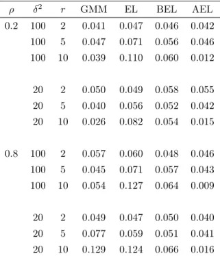
First, Tables 1-3 report the rejection frequencies of four tests at the5%nominal significance level for the cases of normal, standardized t(5), and standardizedχ2(3), respectively. We setn= 200for the sample size, r=2,
5, and 10 for the number of instruments, ρ=0.2 and 0.8 for the degree of endogeneity, and δ2=20 and 100 for
the concentration parameter. Our findings are summarized as follows. First, compared to the nominal level, the rejection frequencies of GMM and EL can be large when the number of moment restrictionsris large. Therefore, in this example the first-order asymptotic approximations for the J-test and its empirical likelihood analog are less precise. Second, improvements by BEL and AEL in the null rejection frequencies are reasonable. For example, in the normal case (Table 1), the rejection frequency varies between .034 and .125 for GMM and between .042 and
4
The version of the J-test statistic considered here isJ= minθ$!ni=1g(Xi,θ)%" & !n i=1g " Xi,θ˜ # g"Xi,θ˜ #"'−1 $!n i=1g(Xi,θ)%,
whereθ˜= arg minθ$!ni=1g(Xi,θ) %"$!n
i=1g(Xi,θ) %
is the GMM estimator with the identity weight matrix (thusθ˜is consistent to estimateθ0and asymptotically normal under Assumptions 1-4). For the linear instrumental variable regression model,θ˜corresponds
to the two-stage least square estimator.
5
To compute the empirical likelihood statistic, Tn = minθ∈Θ2!ni=1log
(
1 +γ(θ)"g(Xi,θ)) where γ(θ) solves !n
i=1
g(Xi,θ)
1+γ!g(Xi,θ) = 0 with respect to γ, we adopted a nested algorithm. For each θ, the computation of γ(θ)
(called the inner loop) is implemented by a quasi-Newton method based on Bruce Hansen’s MATLAB code (available at http://www.ssc.wisc.edu/~bhansen/progs/elikem.zip). For the minimization with respect toθ(called the outer loop), we employed a derivative free optimization algorithm based on thefminsearch function in MATLAB (because θ is scalar for both simulation
.099 for EL, while it varies between .047 and .061 for BEL and between .020 and .053 for AEL. Third, comparing BEL and AEL, BEL shows slightly better performance in the null rejection frequencies particularly when r is large. Based on an inspection of simulation outputs, we conjecture this difference is partly due to the lack of stability of the estimates ofBcto implement AEL (compared to the estimates ofβc to implement BEL). Finally, in general the results are similar for the different distributions of the error terms. For the non-normal cases, all tests generally rejects the null hypothesis slightly more than the normal case.
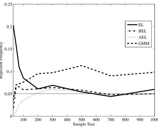
Second, we examine how the rejection frequencies of these tests vary with the sample size. Our theoretical results in Section 3 indicate that the discrepancies between the actual rejection frequencies and the nominal level of BEL and AEL will decay faster than those of GMM and EL as the sample size increases. Figure 1 reports the plots of the rejection frequencies of four tests with the5%nominal level for sample sizesn=30, 50, 70, 100, 200, 500, 700, and 1000 (with r = 5, ρ= 0.8, and δ2 = 20). We can see that as predicted by the theoretical
results, the convergence speeds of the rejection frequencies of BEL and AEL to the nominal5%level are faster than those of GMM and EL. In particular, the convergence speed of the rejection frequency of GMM is slow.
Third, we investigate the null rejection properties of these tests when the concentration parameterδ2is close
to (or equal to) zero, i.e., weak instruments. Although our theoretical analysis focuses on the case of strong identification (i.e., G is full column rank, imposed in Assumption 2), it is important to examine finite sample behaviors of the proposed BEL and AEL tests when the strong identification assumption is questionable. Figure 2 reports the plots of the rejection frequencies of four tests with the5%nominal level forδ2=0, 3, 5, 10, 20, 30,
50, 70, 100, and 200. It is remarkable that the rejection frequency of BEL and AEL are very robust against small non-zero values ofδ2 (ranges between 0.038 and 0.066 for BEL and between 0.034 and 0.061 for AEL). When
δ2= 0, all tests under-reject the null hypothesis. Although it is beyond the scope of this paper, it is interesting
to provide some theoretical explanation on this phenomenon.
Finally, we examine the properties of these overidentifying restriction tests as pre-tests for parameter hypoth-esis testing. We consider a two-stage strategy to test the parameter null hypothhypoth-esisH0P : θ0 = 0. In the first
stage, we test the overidentifying restriction H0. If the null hypothesis H0 is not rejected, we proceed to the
second stage and test the parameter null hypothesisHP
0. Guggenberger and Kumar (2011) provided theoretical
and simulation evidences for the size distortion of this two stage approach in linear instrumental variable regres-sion models. In particular, they derived a lower bound for the asymptotic size of the two stage test and showed that surprisingly the lower bound can be as large as1−α, where αis the nominal size for the first stage test. Although formal analysis is beyond the scope of this paper, it is interesting to investigate finite sample behaviors of this two stage approach when we employ BEL or AEL in the first stage. We compare (i) the J-test followed by the t-test based on the two-step GMM estimator, (ii) the empirical likelihood overidentification test followed by the empirical likelihood ratio test for the parameter hypothesis,6
(iii) the BEL overidentification test followed by the empirical likelihood ratio test for the parameter hypothesis, and (iv) the AEL overidentification test followed by the empirical likelihood ratio test for the parameter hypothesis.
In order to evaluate the asymptotic size of a test forHP
0, we need to analyze the null rejection probabilities
of the test for all possible values of nuisance parameters and find the worst one. It is not easy and beyond the scope of this paper to characterize the asymptotic size property for the two stage test in our simulation design. Thus, after some preliminary simulation studies, we replace the data generating process forYi in (12) with
Yi = Wiθ0+cZ1i+Ui, 6
The empirical likelihood ratio statistic for HP
0 : θ0 = a is defined as TnP = $(a)−minθ∈Θ$(θ). Based on the first-order
where Z1i is the first element of Zi, r = 5, ρ = 0.8, δ2 = 20, andn = 200. By perturbingc from 0, we allow small deviations from the overidentification null hypothesis H0, which corresponds to a nuisance parameter for
testingHP
0. Figure B reports the frequencies of the event “not rejectingH0in the first stage but rejectingH0P in
the second stage”. For both stages, the nominal level is5%. In this particular setup (which does not necessarily characterize the finite sample size of the two stage tests), we can see that the frequencies for this event can be higher than 0.05 for all the two stage tests. The difference among EL, BEL, and AEL-based tests is small.
4.1.2 Power Property
In order to investigate the power properties of the proposes tests, we consider the following data generation process as alternative hypotheses:
Yi = Wiθ0+ 0.1Z1i+Ui,
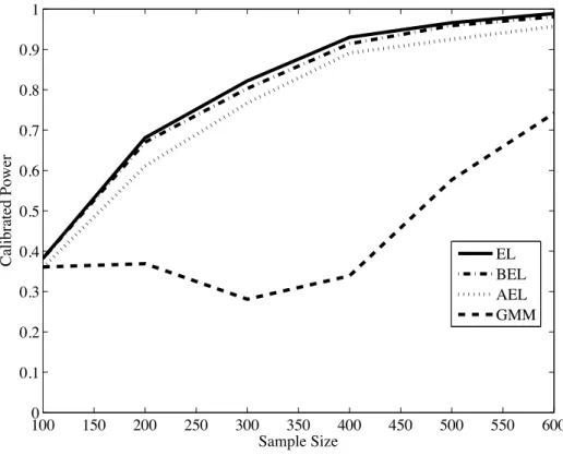
whereZ1i is the first element ofZi, r= 5,ρ= 0.8,δ2 = 20, and n= 200. We can see that there is noθ which satisfiesE[g(Xi,θ)] =E[Zi(Yi−Wiθ)] = 0. We investigate the calibrated powers of GMM, EL, BEL, and AEL (i.e., the rejection frequencies of these overidentification tests where the critical values are given by the Monte Carlo 95%percentiles of these test statistics under the data generation process in (12)). Figure 4 reports the calibrated powers for the tests with sample sizesn= 50, 70, 100, 200, 300, 400, 500, and 600 under the normal case. In this setting, all tests show similar calibrated power properties.
Overall, the simulation results for the linear instrumental variable regression indicate that BEL and AEL have more attractive null properties than EL and GMM and have comparable power properties to EL and GMM.
4.2
Nonlinear Moment Restriction
4.2.1 Performance under the Null Hypothesis
We next consider a simulation design in Liu and Chen (2010) motivated by an asset pricing model, which is a multivariate version of Hall and Horowitz’s (1996) simulation design. Let X = (X1, X2, . . . , Xr)" be a vector
of mutually independent random variables, where X1, X2 ∼N!0,σ2" and X3, . . . , Xr ∼χ2(1). The moment
restrictions are written as
E[g(X,θ0)] =E m(X,θ0) X2m(X,θ0) (X3−1)m(X,θ0) .. . (Xr−1)m(X,θ0) = 0 (13) wherem(X,θ) = exp! −4.5σ2−θ(X
1+X2) + 3X2"−1. We treatσas a given normalizing constant and treat
θas an unknown parameter to be estimated from (13). These restrictions are satisfied atθ0= 3for anyσ>0.7
First, Table 4 reports the rejection frequencies of the four tests at the 5%nominal significance level. We set
σ= 0.2 for the standard deviation of X1 andX2, n= 100and 200for the sample size, andr =2, 3, 5, and 7
for the number of moment restrictions. Our findings are summarized as follows. First, compared to the nominal level, the rejection frequencies of GMM and EL can be quite large particularly when the number of moment
7 Note thatE[m(X,3)] = √1 2πσ2 ´ exp * −(x1+3σ 2 )2 2σ2 +
restrictionsris large. It should be noted that, GMM shows serious distortions in the null rejection frequencies even whenr is as small as 3. Therefore, in this example the first-order asymptotic approximation for the J-test is less precise. Second, improvements by BEL and AEL in the null rejection frequencies are reasonable. The rejection frequency varies between .040 and .370 for GMM and between .054 and .255 for EL, while it varies between .054 and .089 for BEL and between .000 and .052 for AEL. Finally, comparing BEL and AEL, BEL shows better performance in the null rejection frequencies particularly whenr is large. Based on an inspection of simulation outputs, we conjecture this difference is partly due to the lack of stability of the estimates ofBc to implement AEL (compared to the estimates ofβc to implement BEL).
Second, we examine how the rejection frequencies of these tests vary with the sample size. Our theoretical results in Section 3 indicate that the discrepancies between the actual rejection frequencies and the nominal level of BEL and AEL will decay faster than those of GMM and EL as the sample size increases. Figure B reports the plots of the rejection frequencies of four tests with the5%nominal level for sample sizesn=30, 50, 70, 100, 200, 500, 700, and 1000 (withσ = 0.2 andr= 3). We can see that as predicted by the theoretical results, the convergence speeds of the rejection frequencies of BEL and AEL to the nominal5%level are faster than those of GMM and EL. In particular, the convergence speed of the rejection frequency of GMM is slow.
Third, we investigate the null rejection properties of these tests when the matrix G=E%∂g(X,θ0)
∂θ!
&
is close to the zero matrix, i.e., weak identification (Stock and Wright, 2000). Although our theoretical analysis focuses on the case of strong identification (i.e., G is full column rank, imposed in Assumption 2), it is important to examine finite sample behaviors of the proposed BEL and AEL tests when the strong identification assumption is questionable. In order to characterize weak identification in our simulation design, Figure 6 reports the relationship between the constantσand the scalarµ=nG"V−1Gcomputed by Monte Carlo integration. We call
thisµas the degree of concentration since it is analogous to the so-called concentration parameter in the linear instrumental variable regression model. From Figure 6, we can see that µgets smaller asσincreases. Thus, in our setup, large values of σ can be associated with weak identification for the parameter θ0. Figure 7 reports
the plots of the rejection frequencies of four tests with the 5% nominal level forσ =0.1, 0.2, 0.3, 0.4, 0.5, 0.6, 0.7, and 0.8 (withn= 200 andr= 3). Note that all tests over-reject the null hypothesis whenσ is large (i.e., the degree of concentrationµis small). The rejection frequencies of BEL and AEL are closer to the nominal size than those of GMM and EL. In particular, it is remarkable that the rejection frequency of BEL is very robust against large values of σ (ranges between 0.05 and 0.15). Although it is beyond the scope of this paper, it is interesting to provide some theoretical explanation on this phenomenon.
Finally, we examine the properties of these overidentifying restriction tests as pre-tests for parameter hy-pothesis testing. We consider a two-stage strategy to test the parameter null hyhy-pothesis HP
0 : θ0 = 3. In
the first stage, we test the overidentifying restriction H0 in (1). If the null hypothesis H0 is not rejected, we
proceed to the second stage and test the parameter null hypothesis HP
0. Similarly to the previous section, we
compare (i) the J-test followed by the t-test based on the two-step GMM estimator, (ii) the empirical likelihood overidentification test followed by the empirical likelihood ratio test for the parameter hypothesis, (iii) the BEL overidentification test followed by the empirical likelihood ratio test for the parameter hypothesis, and (iv) the AEL overidentification test followed by the empirical likelihood ratio test for the parameter hypothesis.
In order to evaluate the asymptotic size of a test forHP
0, we need to analyze the null rejection probabilities
of the test for all possible values of nuisance parameters and find the worst one. It is not easy and beyond the scope of this paper to characterize the asymptotic size property for the two stage test in our simulation design. Thus, after some preliminary simulation studies, we fix the data generating process asX1, X2∼N
#
X3, . . . , Xr∼χ2(1)withn= 200,σ= 0.2, andr= 3.8 By perturbingc from 1, we allow small deviations from
the overidentification null hypothesisH0, which corresponds to a nuisance parameter for testing H0P. Figure B
reports the frequencies of the event “not rejectingH0in the first stage but rejectingH0P in the second stage”. For
both stages, the nominal level is 5%. In this particular setup (which does not necessarily characterize the finite sample size of the two stage tests), we can see that the frequencies for this event are typically higher than 0.05 for the GMM-based two stage test and lower than 0.05 for the other tests. Also the difference among EL, BEL, and AEL-based tests is small.
4.2.2 Power Property
In order to investigate the power properties of the proposes tests, we consider the two data generation processes as alternative hypotheses: Case 1:X1, X2∼N # 0.05,(0.2)2$, X3∼χ2(1), Case 2:X1, X2∼N # 0,(0.3)2$, X3∼χ2(1).
Under these data generation processes, we specify the moment functions as
g(X,θ) = (m(X,θ), X2m(X,θ),(X3−1)m(X,θ))", where
m(X,θ) = exp#−4.5 (0.2)2−θ(X1+X2) + 3X2
$
−1.
We can see that for both cases, there is noθ which satisfies E[g(X,θ)] = 0. For both cases, we investigate the calibrated powers of GMM, EL, BEL, and AEL (i.e., the rejection frequencies of these overidentification tests where the critical values are given by the Monte Carlo 95%percentiles of these test statistics under the data generation processX1, X2∼N
#
0,(0.2)2$andX3∼χ2(1)satisfyingH0). Figures 9 and 10 report the calibrated
powers with sample sizes n= 100, 200, 300, 400, 500, and 600 for each case. For Case 1, EL, BEL, and AEL show superior calibrated power properties than GMM. For Case 2, EL and BEL have better power than AEL and GMM. Lower calibrated power of GMM is partly due to the over-rejection properties of GMM underH0 as
illustrated in Figure B (which typically yield large critical values to compute calibrated power). For both cases, BEL is slightly less powerful than EL. Since BEL has better null rejection properties than EL (see Figure B), these power properties characterize a trade-offbetween the null rejection and power properties of EL and BEL. For Case 2, AEL tends to have lower calibrated power than BEL and EL, and shows similar properties to GMM. We find that this decay of power in AEL is partly due to the lack of stability of the estimates ofBcto implement AEL.9
Overall, our simulation results are encouraging. BEL and AEL have more attractive null properties than EL and GMM. Based on the power properties, we particularly recommend to use BEL.
5
Conclusion
In this paper, we show that the empirical likelihood test for overidentifying restrictions is Bartlett correctable and propose second-order refinement methods based on the empirical Bartlett correction and adjusted empirical
8
In preliminary analysis, we tried the cases ofX1, X2∼N(
c,σ2)
for different values ofc, different values ofσ(but not too large to avoid weak identification forθ0), and different number of momentsr, for example. The results are basically similar to the one in
Figure B.
9
For example, in Case 2 withn= 200, the bootstrap estimates ofβcandBc range from 0.86 to 3.71 and from -13.73 to 271.18,
likelihood. Simulation results suggest that the empirical Bartlett correction and adjusted empirical likelihood assisted by bootstrapping exhibit better null rejection properties than the conventional GMM and empirical likelihood tests using the first-order asymptotic approximation. It is interesting to extend this research to a time series context and non-smooth moment functions (e.g. quantile instrumental variable regressions).
A
Mathematical Appendix
A.1
Basic Formulae
LetUΛ−1=!ωkl"
p×p. From Chen and Cui (2007), we have the following formulae:
Bk = 0, Bp+a=−Ap+a, Br+k=ωklAl, γj,kBr+k=AjI{j ≤p}, γj,kBj= 0, γj,kBj,l = Cl,k, γj,kBj,p+a = 0, Bk,l Bk,p+b Bk,r+l Bp+a,l Bp+a,p+b Bp+a,r+l Br+k,l Br+k,p+b Br+k,r+l = ωmkCl,m ωmkCp+b,m 0 Alp+a Ap+a p+b −Cp+a,l ωkm! ωnmCl,n −Aml" ωkm! ωnmCp+b,n −Amp+b" ωkmCm,l , βl,p+a p+c = −ωol! γp+c;p+a,o+γp+a;p+c,o" , βl,r+m p+c =ωolγp+c,om, βp+a,p+b p+c= −2αp+a p+b p+c,
βp+a,r+m p+c = γp+c;p+a,m+γp+a;p+c,m, βl,p+a r+n=ωolγp+a,on, βl,r+m r+n = 0,
βp+a,p+b r+n = γp+a,n;p+b+γp+a;p+b,n, βp+a,r+m r+n =−γp+a,mn, βr+k,r+m r+n =ωkoγo,mn,
βr+k,p+a p+c = 2ωkoαop+a p+c−ωkoωno! γp+c;p+a,n+γp+a;p+c,n" , βr+k,p+a r+n = ωkoωmoγp+a,mn−ωko! γo,n;p+a+γo;p+a,n" , βr+k,r+m p+c = ωkoωnoγp+c,nm −ωko! γp+c;o,m+γo,p+c;m" .
A.2
Expression of
R
3 R3p+a is written as R3p+a = ωklωmnCn,kCp+a,mAl+1 2ω klCp+b,kAp+a p+bAl −12ωklωmlCp+a,kCp+b,mAp+b +3 8A p+a p+cAp+b p+cAp+b+ωklCp+b,kAlp+aAp+b + B ωklγp+c;p+d,kαlp+a p+b −12ωklωmlγp+a;p+b,kγp+c;p+d,m +4 9α p+e p+a p+bαp+e p+c p+d −1 4α p+a p+b p+c p+d C Ap+bAp+cAp+d +ωmv ωkl! γp+c;l,m+γl;p+c,m" γp+a;p+b,k+ 3ωklγp+a,kmαlp+b p+c +ωloγp+a;p+b,l(γp+c;o,m+γo;p+c,m−3ωnoγp+a,nm) +αp+d p+a p+b!2 3γ p+d;p+c,m+γp+c;p+d,m" −γp+a;p+b;p+c,m AvAp+bAp+c +ωmvωnv! −1 2ω klωolγp+a,kmγp+b,on+ωklγp+b,km! γl,n;p+a+γl;p+a,n" +1 2ω klγl,mnγp+a;p+b,k+1 3γ p+c,mnαp+a p+b p+c −1 2γ p+a;p+b,mn −1 2γ p+a,m;p+b,n +12γp+a;p+c,m! γp+b;p+c,n+γp+c;p+b,n" +12γp+c;p+a,mγp+b;p+c,n AvAv!Ap+b +1 2ω mvωnv! ωov!!/ ωklωp+a,klωl,mn+γp+b,mnγp+a;p+b,o −13γp+a;m,no 0 AvAv! Av!! −12ωknωloωvmγm,klCp+a,vAnAo−1 4ω knωloγp+b,klAp+b p+aAnAo+ωkmωnmωloγp+a,klCp+b,nAoAp+b −ωkmωloγp+a,klAmp+bAoAp+b−ωkvωlnωmoγp+a,klCv,nAnAo+1 2ω knωloCp+a,klAnAo +1 3A p+a p+b p+cAp+bAp+c+ωlmωnmγp+a;p+b,lCp+c,nAp+bAp+c −ωlmγp+a;p+b,lAmp+cAp+bAp+c −ωlnωmoγp+a;p+b,lCn,mAoAp+b−ωlnωmk! γk;p+a,l+γp+a;k,l" Cp+b,mAnAp+b −ωlnωmoγp+a;p+b,lCp+b,mAnAo− K 1 2γ p+c;p+a,l+γp+a;p+c,l L ωlnAp+b p+cAnAp+b +ωlmCp+a;p+b,lAmAp+b−ωmkαkp+a p+bCp+c,mAp+bAp+c −23ωlmαp+a p+b p+cCp+c,lAmAp+b−5 6α p+a p+b p+cAp+c p+dAp+bAp+d. (14)A.3
Derivation of
R
3 We first evaluate the terms in *6j=3Lj+ *11 j=10Lj+ *23 j=13Lj+ *33
j=25Lj. Note that the termsL5, L6,L11,
L19, andL22 cancel each other since
βj,uq1
−Br+k,sBsγj,k+Cj,kBr+k+Bj,sBs−AjiBi2
BuBq = 0, from the formulae in Appendix A.1. The other terms are written as follows.
L3+L10+L17+L21
= 2ωklωmnCn,kCp+a,mAlAp+a+ 2ωklCp+b,kAp+a p+bAlAp+a+ωklωmnCp+a,kCp+a,mAlAn
L4 = − 1 2ω kl! γp+b;p+a,k+γp+a;p+b,k" 1 2αlp+cp+d−ωml! γp+d;p+c,m+γp+c;p+d,m"2 Ap+aAp+bAp+cAp+d +ωklωmo! γp+a;p+c,k+γp+c;p+a,k" 1ωnlγp+b,nm−! γl,m;p+b+γl;p+b,m"2 AoAp+aAp+bAp+c +ωklωmoγp+a,km1 2αlp+b p+c−ωnl! γp+c;p+b,n+γp+b;p+c,n"2 AoAp+aAp+bAp+c +2ωklωmvωnv!γp+a,km1 ωolγp+b,on−! γl,n;p+b+γl;p+b,n"2 AvAv!Ap+aAp+b −12ωklωmoωnv! γp+b;p+a,k+γp+a;p+b,k" γl,mnAoAvAp+aAp+b−ωklγp+a,kmγl,mnωmvAvωnv!Av!ωov!!Av!!Ap+a. L13 = −ωknωloωvmγm,klCp+a,vAnAoAp+a−ωknωloγp+b,klAp+b p+aAnAoAp+a −ωkmωloωnvγp+a,klCp+b,nAmAoAv+ 2ωkmωlo! ωnmCp+b,n−Amp+b" γp+a,klAoAp+aAp+b −2ωkvωlnωmoγp+a,klCv,mAnAoAp+a. L14 = 1 2ω omωknωlvγm,kl! γp+b;p+a,o+γp+a;p+b,o" AnAvAp+aAp+b+ωkmωlnγp+c,klαp+a p+b p+cAmAnAp+aAp+b +ωomωkvωlv! ωnv!! γm,klγp+a,onAvAv! Av!! Ap+a+ωkmωloωnvγp+b,kl! γp+b,n;p+a+γp+b;p+a,n" AmAoAvAp+a +1 2ω koωlvωmv! ωnv!! γp+a,klγp+a,mnAoAvAv! Av!! +ωkoωlvωmv! ωnv!! γp+a,klγo,mnAvAv! Av!! Ap+a +ωkoωlvγp+a,kl{2αop+b p+c−ωno! γp+c;p+b,n+γp+b;p+c,n" }AvAp+aAp+bAp+c −2ωkoωlvωnv!γp+a,kl1 ωmoγp+b,mn−! γo,n;p+b+γo;p+b,n"2 AvAv!Ap+aAp+b. L15+L16=ωknωloCp+a,klAnAoAp+a+ 2 3A p+a p+b p+cAp+aAp+bAp+c. L18 = −1 4ω okωo!k! γp+b;p+a,o+γp+a;p+b,o"# γp+d;p+c,o!+γp+c;p+d,o!$Ap+aAp+bAp+cAp+d −ωokωo!kωlm! γp+b;p+a,o+γp+a;p+b,o" γp+c,o!lAmAp+aAp+bAp+c −ωokωo!kωlnωmvγp+a,olγp+b,o!mAnAvAp+aAp+b−αp+e p+a p+bαp+e p+c p+dAp+aAp+bAp+cAp+d −2ωlm! γp+d,l;p+c+γp+d;p+c,l" αp+d p+a p+bAmAp+aAp+bAp+c −αp+c p+a p+bγp+c,lmωlnωmoAnAoAp+aAp+b −ωlnωmo! γp+c,l;p+a+γp+c;p+a,l" ! γp+c,m;p+b+γp+c;p+b,m" AnAoAp+aAp+b −ωloωmvωnv!! γp+b,l;p+a+γp+b;p+a,l" γp+b,mnAoAvAv!Ap+a −14ωlvωmv!ωnv!!ωov!!!γp+a,lmγp+a,noAvAv!Av!!Av!!!. L20+L23=−2ωklγp+a;p+b;p+c,kAlAp+aAp+bAp+c− 1 3ω knωloωmvγp+a;k,lmAnAoAv. L25 = 2ωlmγp+a;p+b,l ! ωnmCp+c,n−Am,p+c" Ap+aAp+bAp+c−2ωlnωmoγp+a;p+b,lCn,mAoAp+aAp+b.
L26 = ωloγp+a;p+b,l12αop+c p+d−ωno!γp+d;p+c,n+γp+c;p+d,n"2Ap+aAp+bAp+cAp+d −2ωloωmvγp+a;p+b,l1 ωnoγp+c,nm−! γp+c;o,m+γo;p+c,m"2 AvAp+aAp+bAp+c +ωloωmvωnv! γp+a;p+b,lγo,mnAvAv! Ap+aAp+b. L27 = −2ωlnωmkγk;p+a,lCp+b,mAnAp+aAp+b−2ωlnγp+c;p+a,lAp+c p+bAnAp+aAp+b −2ωlnωmoγp+b;p+a,lCp+b,mAnAoAp+a−2ωlnωmkγp+a;k,lCp+b,mAnAp+aAp+b −2ωlnγp+a;p+b,lAp+b p+cAnAp+aAp+c−2ωlnωmoγp+a;p+b,lAnAoCp+b,mAp+a. L28 = ωokωlmγk;p+a,l! γp+c;p+b,o+γp+b;p+c,o" AmAp+aAp+bAp+c+ 2ωokωmnωloγk;p+d,lγp+a,omAnAoAp+dAp+a +2ωlmγp+d;p+a,lαp+d p+b p+cAmAp+aAp+bAp+c+ 2ωmnωloγp+c;p+a,l! γp+c,m;p+b+γp+c;p+b,m" AnAoAp+aAp+b +γp+b;p+a,lγp+b,mnωmoωnvωlv!AoAvAv!Ap+a+γp+a;k,lωokωlm! γp+c;p+b,o+γp+b;p+c,o"AmAp+aAp+bAp+c +2ωokωmnωloγp+a;k,lγp+b,omAnAoAp+aAp+b+ 2ωlmγp+a;p+b,lαp+b p+c p+dAmAp+aAp+cAp+d +2ωmnωloγp+a;p+b,l! γp+b,m;p+c+γp+b;p+c,m" AnAoAp+aAp+c+ωmoωnvωlv!γp+a;p+b,lγp+b,mnAoAvAv!Ap+a. L29+L30= 2ωlmCp+a;p+b,lAmAp+aAp+b−ωlmωkn!γp+a;p+b,lk+γp+a,l;p+b,k"AmAnAp+aAp+b. L31 = −2ωmkαkp+a p+bCp+c,mAp+aAp+bAp+c−2αp+a p+b p+cAp+c p+dAp+aAp+bAp+d −2ωlmαp+a p+b p+cCp+c,lAmAp+aAp+b.
L32 = ωokαkp+a p+b!γp+d;p+c,o+γp+c;p+d,o"Ap+aAp+bAp+cAp+d+ 2ωokωlmαkp+a p+bγp+c,olAmAp+aAp+bAp+c
+2αp+e p+a p+bαp+b p+c p+dAp+aAp+bAp+cAp+d+ωlnωmoγp+c,lmαp+c p+a p+bAnAoAp+aAp+b +2ωlm! γp+d,l;p+c+γp+d;p+c,l" αp+d p+a p+bAmAp+aAp+bAp+c. L33=−1 2α p+a p+b p+c p+dAp+aAp+bAp+cAp+d.
Combining these results, we obtain the expression for*6 j=3Lj+ *11 j=10Lj+ *23 j=13Lj+ *33 j=25Lj. By subtracting R2p+aR p+a
2 from this expression, we obtain2R
p+a
3 R
p+a
1 , which yields the expression ofR
p+a
3 in (14).
A.4
Second-order Cumulant of
R
In this subsection, let “[2]” mean “[2, a, f]” fora, f ∈{1, . . . , r−p}. Observe that cum! Rp+a, Rp+f" =E' Rp+aRp+f( −E' Rp+a( E' Rp+f( = n−1δp+a p+f+E%Rp2+aR p+f 2 & +E%Rp2+aR p+f 1 & [2] +E%Rp3+aR p+f 1 & [2]−n−2µp+aµp+f +O! n−3" . (15)
The second term of (15) is n2E%Rp2+aR p+f 2 & = 1 4α p+a p+f p+b p+b −367 αp+a p+b p+cαp+f p+b p+c+ 1 36α p+a p+b p+bαp+f p+c p+c −14δp+a p+f +ωkl K 1 6γ p+a,k;lαp+f p+b p+b[2] +1 2γ p+a,k;p+bαlp+f p+b[2] −12γp+b,k;p+aαlp+f p+b[2] L +ωkmωlm K γp+a,k;p+f,l−γp+b,l;p+aγp+f,k;p+b[2] +γp+b,l;p+aγp+b,k;p+f−121 γp+a,klαp+f p+b p+b[2] L +ωklωmn! γp+a,k;lγp+f,m;n+γp+a,k;nγp+d,m;l" +ωklωmnωk1n K −12γp+a,k;lγp+f,mk1[2]−γp+a,kk1γp+f,m;l[2] L +1 4 ! ωkmωlmωk1m1ωl1m1+ωkmωlnωk1mωl1n+ωkmωlnωk1nωl1m"γp+a,klγp+f,k1l1+O! n−1" . The third term of (15) is
n2E%Rp2+aRp1+f& = −1 2α p+a p+b p+b p+f+1 2δ p+a p+bδp+b p+f+1 3α p+a p+b p+cαp+b p+c p+f −γl;p+f;p+a,kωkl+1 2γ p+a,klωkmωlnαmnp+f+γp+a;p+b,lωlmαmp+b p+f+O! n−1" .
The fourth term of (15) is n2E%Rp3+aR p+f 1 & = ωklωmn! γn,k;p+fγp+a,m;l+γn,k;lγp+a,m;p+f" +1 2 ! γp+b,k;lαp+a p+b p+f+γp+b,k;p+fαp+a p+b l" −12ωklωml!
γp+a,k;p+f,m+γp+a,k;p+bγp+b,m;p+f+γp+a,k;p+fγp+b,m;p+b"
+3 8 ! αp+a p+c p+c p+f+αp+a p+b p+cαp+b p+c p+f+αp+a p+c p+fαp+b p+b p+c−δp+a p+f" +ωkl! γp+f,k;p+a,l+γp+b,k;p+bαlp+a p+b+γp+b,k;p+fαlp+a p+b" +ωkl! γp+b;p+f,k+γp+f;p+b,k" αlp+a p+b+ωklγp+c;p+c,kαlp+a p+f −12ωklωmlγp+a;p+b,k! γp+b;p+f,m+γp+f;p+b,m" −12ωklωmlγp+a;p+f,kγp+c;p+c,m +8 9α p+a p+b p+eαp+b p+e p+f+4 9α p+a p+e p+fαp+c p+c p+e −34αp+a p+b p+b p+f +ωmvωnv −1 2ωklωnlγp+a,kmγp+f,on+ωklγp+f,km ! γl,m;p+a+γl;p+a,m" +12ωklγl,mnγp+a;p+f,k+1 3α p+a p+f p+cγp+c,mn −12γ p+a;p+f,mn −12γ p+a,m;p+f,n +1 2γ p+a;p+c,m! γp+f;p+c,n+γp+c;p+f,n" +1 2γ p+c;p+a,mγp+f;p+c,n −12ωknωlnωvmγm,klγp+a,v;p+f+1 4ω knωlnγp+b,klαp+a p+b p+f +ωkmωnmωloγp+a,klγp+f,n;o
−ωknωloγp+a,klαmop+f−ωkvωlnωmnγp+a,klγv,n;p+f+1
2ω knωlnγp+a,kl;p+f+αp+a p+b p+b p+f +ωlmωnm1 γp+a;p+b,l! γp+f,n;p+b+γp+b,n;p+f" +γp+a;p+f,lγp+c,n;p+c2 −2ωlm! γp+a;p+b,lαmp+b p+f+γp+a;p+f,lαmp+c p+c" −ωlnωmoγp+a,p+f,lγn,m;o −ωlnωmk! γk;p+a,l+γp+a;k,l" γp+f,m;n−ωlnωmnγp+a;p+b,lγp+b,m;p+f −12ωln! γp+c;p+a,l+γp+a;p+c,l" αnp+f p+c+ωlmγp+a;p+f,l;m −ωmk1 αkp+a p+b! γp+f,m;p+b+γp+b,m;p+f" +αkp+a p+fγp+c,m;p+c2 −23ωlmγp+c,l;mαp+a p+f p+c −56! 2αp+a p+b p+cαp+b p+c p+f+αp+a p+f p+cαp+c p+d p+d" +O! n−1" . Combining these results,
cum! Rp+a, Rp+f" =n−1δp+a p+f+n−2∆p+a p+f +O! n−3" , where ∆p+a p+f = 1 2α p+a p+f p+b p+b −13αp+a p+b p+cαp+f p+b p+c− 1 36α p+a p+f p+cαp+b p+b p+c +ωklγl;p+f;p+a,k[2]−1 2ω kmωlnγp+a,klαm n p+f[2] +ωlm K γp+b;p+b,lαm p+a p+f−1 2γ p+f;p+b,lαm p+a p+b L [2] +ωkmωlm K −γp+a,k;p+f,l+1 6γ p+b,klαp+a p+f p+b L −13ωklγp+b,k;lαp+a p+f p+b−ωklγp+a;p+f,kαl p+b p+b[2] +ωklωmnωvnγp+a,v;lγp+f,km[2] −12ωkmωlnωk!mωl!nγp+a,klγp+f,k!l!+ωklωmlγp+a;p+b,kγp+b,m;p+f.
A.5
Third-order Cumulant of
R
Using the results to derive the first and second-order cumulants, the third-order cumulant is written as cum! Rp+a, Rp+b, Rp+d" = E' Rp+aRp+bRp+d( −E' Rp+a( E' Rp+bRp+d( [3] + 2E' Rp+a( E' Rp+b( E' Rp+d( = E%R1p+aR p+b 1 R p+d 1 & −E' Rp2+a ( E%Rp1+bR p+d 1 & [3] +E%Rp2+aR p+b 1 R p+d 1 & [3] +O! n−3" , (16) whereE[Rp+a]E' Rp+bRp+d( [3] =E[Rp+a]E' Rp+bRp+d( +E' Rp+b( E' Rp+aRp+d( +E' Rp+d( E' Rp+aRp+b( and other terms are similarly defined. The first term of (16) is
n2E%Rp+a 1 R p+b 1 R p+d 1 & =αp+a p+b p+d+O! n−1" . The second term of (16) is
n2E' Rp2+a( E%Rp1+bRp1+d&=− /1 6α p+a p+b1 p+b1+ωklγl;p+a,k −12γp+a,klωkmωlm 0 δp+b p+d+O! n−1" . The third term of (16) is
n2E%R2p+aR1p+bRp1+d& = −1 3α p+a p+b p+d −16αp+a p+b1 p+b1δp+b p+d −ωklγp+a,k;lδp+b p+d+1 2γ p+a,klωkmωlnδmnδp+b p+d+O! n−1" . Combining these results, we obtaincum!
Rp+a, Rp+b, Rp+d"
=O!
n−3" .
A.6
Fourth-order Cumulant of
R
In this subsection, let
t1 = αp+a p+b p+c p+d
t2 = δp+a p+bδp+c p+d+δp+a p+cδp+b p+d+δp+a p+dδp+b p+c,
t3 = αp+a p+b1 p+b1αp+b p+c p+d+αp+b p+b1 p+b1αp+a p+c p+d,
+αp+c p+b1 p+b1αp+a p+b p+d+αp+d p+b1p+b1αp+a p+b p+c,
t4 = αp+a p+b p+b1αp+c p+d p+b1+αp+a p+c p+b1αp+b p+d p+b1+αp+a p+d p+b1αp+b p+c p+b1.
Using the results to obtain the first, second, and third-order cumulants,
cum! Rp+a, Rp+b, Rp+c, Rp+d" = E' Rp+aRp+bRp+cRp+d( −E' Rp+aRp+b( E' Rp+cRp+d( [3]−E' Rp+a( E' Rp+bRp+cRp+d( [4] +2E' Rp+a( E' Rp+b(E' Rp+cRp+d([6]−6E' Rp+a( E' Rp+b(E' Rp+c(E' Rp+d( = E%Rp1+aR p+b 1 R p+c 1 R p+d 1 & −E%Rp1+aR p+b 1 & E%Rp1+cR p+d 1 & [3] +E%R2p+aR p+b 1 R p+c 1 R p+d 1 & [4] −E%R2p+aR p+b 1 & E%Rp1+cR p+d 1 & [12] +E%R2p+aR p+b 2 R p+c 1 R p+d 1 & [6]−E%Rp2+aR p+b 2 & E%Rp1+cR p+d 1 & [6] +E%R3p+aR p+b 1 R p+c 1 R p+d 1 & [4]−E%Rp3+aR p+b 1 & E%Rp1+cR p+d 1 & [12]−E' Rp2+a ( E%Rp1+bR p+c 1 R p+d 1 & [4] −E' Rp2+a ( E%Rp2+bR p+c 1 R p+d 1 & [12] + 2E' R2p+a ( E%Rp2+b & E%R1p+cR p+d 1 & [6] +O! n−4" . (17)
The first term of (17) is n3E%R1p+aR p+b 1 R p+c 1 R p+d 1 & =αp+a p+b p+c p+d+O! n−1" . The second term of (17) is
n3E%Rp1+aR p+b 1 & E%Rp1+cR p+d 1 & [3] =δp+a p+bδp+c p+d+δp+a p+cδp+b p+d+δp+a p+dδp+b p+c+O! n−1" . The third and fourth terms of (17) are
n3E%Rp2+aR p+b 1 R p+c 1 R p+d 1 & [4]−n3E%Rp2+aR p+b 1 & E%Rp1+cR p+d 1 & [12] = −6t1+ 2t2− 1 6t3+ 2 3t4+ 1 2γ p+a,klωkmωlmαp+b p+c p+d[4] −ωkl1
γp+a,k;lαp+b p+c p+d+γp+a,k;p+bαlp+c p+d+γp+a,k;p+cαlp+b p+d+γp+a,k;p+dαlp+b p+c2 [4] +1 γp+a;p+d,lωlmαmp+b p+c+γp+a;p+c,lωlmαmp+b p+d+γp+a;p+b,lωlmαmp+c p+d2 [4] +O! n−1" . The fifth and sixth terms of (17) are
n3E%Rp2+aR p+b 2 R p+c 1 R p+d 1 & [6]−n3E%Rp2+aR p+b 2 & E%R1p+cR p+d 1 & [6] = 3t1−t2+ 1 6t3− 5 9t4+ 1 3ω kl! γp+a,k;lαp+b p+c p+d+γp+b,k;lαp+a p+c p+d" [6] +1 2ω kl! γp+a,k;p+cαlp+b p+d+γp+a,k;p+dαlp+b p+c+γp+b,k;p+cαlp+a p+d+γp+b,k;p+dαlp+a p+c+" [6] −12ωkl! γp+c,k;p+aαlp+b p+d+γp+c,k;p+bαlp+a p+d+γp+d,k;p+aαlp+b p+c+γp+d,k;p+bαlp+a p+c" [6] +ωklωml! γp+a,k;p+cγp+b,m;p+d+γp+a,k;p+dγp+b,m;p+c+γp+c,k;p+aγp+d,m;p+b+γp+d,k;p+aγp+c,m;p+b" [6] −ωklωml! γp+a,k;p+cγp+d,m;p+b+γp+a,k;p+dγp+c,m;p+b+γp+c,k;p+aγp+b,m;p+d+γp+d,k;p+aγp+b,m;p+c" [6] −16ωkmωlm! γp+a,klαp+b p+c p+d+γp+b,klαp+a p+c p+d" [6] +O! n−1" . The seventh and eighth terms of (17) are
n3E%R3p+aR p+b 1 R p+c 1 R p+d 1 & [4]−n3E%Rp3+aR p+b 1 & E%R1p+cR p+d 1 & [12] = 2t1−1 9t4+O ! n−1" . Using the results to derive the first, second, and third cumulants, the last three terms of (17) are of orderO!
n−4" . Combining these results, we obtaincum!
Rp+a, Rp+b, Rp+c, Rp+d"
=O!
n−4" .
A.7
Proof of Theorem 3.1
In Section 3.1, we have
n−1Tn= (R1+R2+R3)p+a(R1+R2+R3)p+a+Op
#
n−5/2$,
whereR1,R2 andR3are given by (3), (4) and (14), respectively. The first four cumulants ofR=R1+R2+R3
are given by (6), (7) and (8), respectively.
Once we expand n−1Tn in (2) and compute its cumulants, the derivation of an Edgeworth expansion for the
A.8
Proof of Theorem 3.2
The proof is similar to that of Chen and Cui (2007, Theorem 3). Pick anyt∈R. Theorem 3.1 (i) implies Pr{Tn≤t}=Fr−p(t)−n−1tfr−p(t)Bc+O!n−2",
whereFr−pis the cumulative distribution function of theχ2(r−p)distribution. LetTn∗be a bootstrap resample of Tn using the implied probabilities {piˆ}ni=1 in (10). By applying the same argument in Brown and Newey (2002, pp. 510-511) (i.e., applying the same argument for Theorem 3.1 (i) to T∗
n given the original sample
Xn= (X1, . . . , Xn)), we can obtain Pr{Tn∗< t|Xn}=Fr−p(t)−n−1Bˆc∗tfr−p(t) +Op ! n−2" , (18) where Bˆ∗
c is a bootstrap counterpart of Bc obtained by replacing all population moments with the weighted averages based on{piˆ}ni=1 . Since (i) βˆc is a simulation estimator ofE[Tn∗|Xn] (where the error by simulation is asymptotically negligible for suitably chosenB), (ii)(r−p)−1E[T∗
n|Xn] = 1 +n−1Bˆc∗+Op ! n−3/2" by (18), and (iii)Bˆ∗ c =Bc+Op ! n−1/2"
by Brown and Newey (2002, Theorem 1), we obtain ˆ
βc = 1 +n−1Bc+Op
#
n−3/2$.
Therefore, an application of the delta method (Hall, 1992, Section 2.7) yields Pr3Tn< cαβˆc 4 = Pr1 Tn < cα ! 1 +n−1Bc"2 +O#n−3/2$= 1−α+O#n−3/2$.
B
Tables and Figures
ρ δ2 r GMM EL BEL AEL 0.2 100 2 0.049 0.057 0.053 0.045 100 5 0.041 0.054 0.048 0.040 100 10 0.037 0.099 0.058 0.031 20 2 0.039 0.042 0.049 0.041 20 5 0.040 0.051 0.056 0.047 20 10 0.034 0.075 0.049 0.031 0.8 100 2 0.045 0.047 0.053 0.048 100 5 0.051 0.068 0.053 0.047 100 10 0.047 0.092 0.055 0.027 20 2 0.062 0.048 0.047 0.037 20 5 0.095 0.061 0.061 0.053 20 10 0.125 0.080 0.050 0.020Table 1: Rejection frequencies of tests at 5% level with n= 200(normal case)
ρ δ2 r GMM EL BEL AEL 0.2 100 2 0.041 0.047 0.046 0.042 100 5 0.047 0.071 0.056 0.046 100 10 0.039 0.110 0.060 0.012 20 2 0.050 0.049 0.058 0.055 20 5 0.040 0.056 0.052 0.042 20 10 0.026 0.082 0.054 0.015 0.8 100 2 0.057 0.060 0.048 0.046 100 5 0.045 0.071 0.057 0.043 100 10 0.054 0.127 0.064 0.009 20 2 0.049 0.047 0.050 0.040 20 5 0.077 0.059 0.051 0.041 20 10 0.129 0.124 0.066 0.016
ρ δ2 r GMM EL BEL AEL 0.2 100 2 0.048 0.056 0.058 0.052 100 5 0.042 0.076 0.062 0.044 100 10 0.032 0.126 0.060 0.013 20 2 0.046 0.047 0.056 0.053 20 5 0.035 0.058 0.048 0.044 20 10 0.039 0.092 0.057 0.019 0.8 100 2 0.055 0.061 0.057 0.052 100 5 0.049 0.077 0.054 0.041 100 10 0.048 0.125 0.063 0.011 20 2 0.058 0.051 0.051 0.044 20 5 0.082 0.084 0.064 0.053 20 10 0.139 0.129 0.066 0.015
Table 3: Rejection frequencies of tests at 5% level with n= 200(standardizedχ2(3)case)
n r GMM EL BEL AEL 100 2 0.040 0.063 0.056 0.052 3 0.135 0.105 0.074 0.047 5 0.244 0.161 0.077 0.016 7 0.370 0.255 0.087 0.000 200 2 0.048 0.054 0.054 0.052 3 0.106 0.069 0.057 0.048 5 0.243 0.114 0.072 0.035 7 0.326 0.167 0.089 0.008
100 200 300 400 500 600 700 800 900 1000 0 0.05 0.1 0.15 0.2 0.25 Sample Size Rejection Frequency EL BEL AEL GMM
Figure 1: Rejection frequencies for different values of sample sizes with r= 5,ρ= 0.8, andδ2= 20
0 20 40 60 80 100 120 140 160 180 200 0 0.05 0.1 0.15 δ2 Rejection Frequency EL BEL AEL GMM
−00.2 −0.15 −0.1 −0.05 0 0.05 0.1 0.15 0.2 0.05 0.1 0.15 c Rejection Frequency EL BEL AEL GMM
Figure 3: Frequencies of the event “not reject in the first stage but reject in the second stage” withr= 5,ρ= 0.8, δ2= 20, andn= 200 50 100 150 200 250 300 350 400 450 500 550 600 0 0.1 0.2 0.3 0.4 0.5 0.6 Sample Size Calibrated Power EL BEL AEL GMM
30 100 200 300 400 500 600 700 800 900 1,000 0 0.05 0.1 0.15 0.2 Sample Size Rejection Frequency EL BEL AEL GMM
Figure 5: Rejection frequencies for different sample sizes withσ= 0.2and r= 3
0.1 0.2 0.3 0.4 0.5 0.6 0.7 0.8 4 8 12 16 20 24 28 σ Degree of Concentration
0.1 0.2 0.3 0.4 0.5 0.6 0.7 0.8 0 0.05 0.1 0.2 0.3 0.4 0.5 0.6 0.7 0.8 σ Rejection Frequency EL BEL AEL GMM
Figure 7: Rejection frequencies for different values ofσ withn= 200andr= 3
0.5 0.6 0.7 0.8 0.9 1 1.1 1.2 1.3 1.4 1.5 0 0.05 0.1 0.15 0.2 c Rejection Frequency EL BEL AEL GMM
Figure 8: Frequencies of the event “not reject in the first stage but reject in the second stage” with n = 200,
1000 150 200 250 300 350 400 450 500 550 600 0.1 0.2 0.3 0.4 0.5 0.6 0.7 0.8 0.9 1 Sample Size Calibrated Power EL BEL AEL GMM
Figure 9: Calibrated power for Case 1
1000 150 200 250 300 350 400 450 500 550 600 0.1 0.2 0.3 0.4 0.5 0.6 0.7 0.8 0.9 1 Sample Size Calibreated Power EL BEL AEL GMM