Biological Systems Engineering--Dissertations,
Theses, and Student Research Biological Systems Engineering
12-2017
High Throughput Phenotyping of Sorghum for the
Study of Growth Rate, Water Use Efficiency, and
Chemical Composition
Piyush Pandey
University of Nebraska-Lincoln, [email protected]
Follow this and additional works at:http://digitalcommons.unl.edu/biosysengdiss Part of theBioresource and Agricultural Engineering Commons
This Article is brought to you for free and open access by the Biological Systems Engineering at DigitalCommons@University of Nebraska - Lincoln. It has been accepted for inclusion in Biological Systems Engineering--Dissertations, Theses, and Student Research by an authorized administrator of DigitalCommons@University of Nebraska - Lincoln.
Pandey, Piyush, "High Throughput Phenotyping of Sorghum for the Study of Growth Rate, Water Use Efficiency, and Chemical Composition" (2017).Biological Systems Engineering--Dissertations, Theses, and Student Research. 74.
HIGH THROUGHPUT PHENOTYPING OF SORGHUM FOR THE STUDY OF GROWTH RATE, WATER USE EFFICIENCY, AND CHEMICAL COMPOSITION
by
Piyush Pandey
A THESIS
Presented to the Faculty of
The Graduate College at the University of Nebraska
In Partial Fulfillment of Requirements
For the Degree of Master of Science
Major: Agricultural and Biological Systems Engineering
Under the Supervision of Professor Yufeng Ge
Lincoln, Nebraska
HIGH THROUGHPUT PHENOTYPING OF SORGHUM FOR THE STUDY OF GROWTH RATE, WATER USE EFFICIENCY, AND CHEMICAL COMPOSITION
Piyush Pandey, M.S.
University of Nebraska, 2017
Advisor: Yufeng Ge
Plant phenotyping using digital images has increased the throughput of the trait
measurement process, and it is considered to be a potential solution to the problem of the phenotyping bottleneck. In this study, RGB images were used to study relative growth rate (RGR) and water use efficiency (WUE) of a diverse panel of 300 sorghum plants of 30 genotypes, and hyperspectral images were used for chemical analysis of
macronutrients and cell wall composition. Half of the plants from each genotype were subjected to drought stress, while the other half were left unstressed. Quadratic models were used to estimate the shoot fresh and dry weights from plant projected area. RGR values for the drought-stressed plants were found to gradually lag behind the values for the unstressed plants. WUE values were highly variable with time. Significant effects of drought stress and genotype were observed for both RGR and WUE. Hyperspectral image data (546 nm to 1700 nm) were used for chemical analysis of macronutrients (N, P, and K), neutral detergent fiber (NDF), and acid detergent fiber (ADF) for plant samples separated into leaf and three longitudinal sections of the stem. The accuracy of the models built using the spectrometer data (350 nm to 2500 nm) of dried and ground biomass was found to be higher than the accuracy of models built using the image data.
1.46) were found to be satisfactory for quantitative analysis whereas the models for K, NDF, and ADF were not suitable for quantitative prediction. Models built after the separation of leaf and stem samples showed variation in the accuracy between the two groups. This study indicates that image-based non-destructive analysis of plant growth rate and water use efficiency can be used for studying and comparing the effects of drought across multiple genotypes. It also indicates that two dimensional hyperspectral imaging can be a useful tool for non-destructive analysis of chemical content at the tissue level, and potentially at the pixel level.
Keywords: high throughput phenotyping, hyperspectral images, RGB images, growth rate, chemical analysis
ACKNOWLEDGMENTS
I would like to express my gratitude towards my advisor Dr. Yufeng Ge for the constant guidance and inspiration he has provided throughout my study and research. I also thank him for all the motivation, and for the great patience with which he has advised me.
I would also like to thank my thesis committee members: Dr. James Schnable, Dr. Jeyamkondan Subbiah, and Dr. Sibel Irmak for their excellent comments, instructions, and encouragement for my work on both my research and my thesis.
Thanks are also due to my labmates Abbas Atefi, Geng Bai, Nuwan Wijewardane, Suresh Thapa, Ujjwol Bhandari, and Wenan Yuan for their help on everything from planting seeds and collecting data to giving me good ideas in general. I am also thankful to Vincent Stoerger and Troy Pabst for their help in running the experiment in the phenotyping greenhouse.
And finally, I would like to thank my parents for everything they have done for me.
TABLE OF CONTENTS
ABSTRACT ... ii
ACKNOWLEDGMENTS ... iv
TABLE OF CONTENTS ...v
LIST OF FIGURES ... viii
LIST OF TABLES ... xi
CHAPTER 1 ... 1
1.1 PHENOTYPING FOR PLANT BREEDING ... 1
1.2 HIGH THROUGHPUT PLANT PHENOTYPING ... 3
1.3 DIGITAL IMAGING MODULES ... 3
1.3.1 Phenotyping using RGB images ... 5
1.3.2 Phenotyping using hyperspectral images ... 6
1.4 HIGH THROUGHPUT CHEMICAL PHENOTYPING OF SORGHUM ... 8
1.4.1 Cell wall characterization ... 9
1.4.2 Nutrient analysis ... 10
1.5 OBJECTIVES OF THE STUDY ... 12
CHAPTER 2 ... 13
2.2 DATA COLLECTION ... 15
2.3 CHEMICAL DATA ... 16
2.4 RGB IMAGE PROCESSING ... 17
2.4.1 Image segmentation... 17
2.4.2 Relative growth rate and water use efficiency ... 20
2.5 HYPERSPECTRAL IMAGES ... 22
2.5.1 Image acquisition ... 22
2.5.2 Segmentation ... 23
2.5.3 Chemometric models... 24
CHAPTER 3 ... 27
3.1 SHOOT FRESH WEIGHT ... 27
3.2 ESTIMATION OF FRESH SHOOT WEIGHT FROM RGB IMAGES ... 29
3.3 ESTIMATION OF SHOOT DRY WEIGHT ... 33
3.4 RELATIVE GROWTH RATE ANALYSIS ... 33
3.5 CLIMATE DATA ... 36
3.6 WATER USE EFFICIENCY ... 39
3.7 RANKING OF GENOTYPES ... 42
3.9 PLSR MODELING WITH SPECTROMETER DATA ... 44
3.10 PLSR MODELING WITH IMAGE DATA ... 53
3.11 PLSR WITH RESAMPLED SPECTROMETER DATA ... 57
CHAPTER 4 ... 60
LIST OF FIGURES
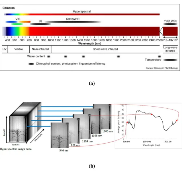
Figure 1.1 (a) The electromagnetic spectrum and imaging modules (Source: Fahlgren, Gehan, & Baxter, 2015) (b) Hyperspectral images shown as a cube of images that are individually processed to extract the spectrum of pixel intensities ... 4 Figure 2.1 The sequential steps in segmentation of plant pixels from the background; the
upper left panel shows the initial RGB image; the upper right panel shows the result after thresholding with the color index; the lower left image results after the
morphological opening, and the lower right image is the final mask after removing the vertical stripe using algorithm based on eccentricity and orientation ... 19 Figure 2.2 Setup of the hyperspectral imaging chamber ... 22 Figure 2.3. Flowchart showing the steps in hyperspectral image segmentation ... 25 Figure 3.1. (a) Boxplots demonstrating the distribution of fresh shoot weights in the
drought stressed group D and control group C (b) Distribution of the average area in square millimeters covered by plant pixels on the RGB images; the areas from five side view images have been averaged ... 27 Figure 3.2. Boxplots demonstrating the distribution of fresh shoot weights in the drought
stressed and control groups for each genotype in the experiment ... 28 Figure 3.3. Correlation between total shoot fresh weight and the sum of area occupied by
plant pixels in the five side view images. ... 29 Figure 3.4. Correlation between total shoot fresh weight and the sum of area occupied by
Figure 3.5. Correlation diagram for plants belonging to the line "E1" The plants in the control group are denoted by "C" whereas the plants in the drought group are
denoted by "D" ... 31 Figure 3.6. Correlation between total shoot fresh weight and the sum of area occupied by
plant pixels for plants with emerged head during sampling ... 32 Figure 3.7. Shoot fresh weight and aggregated area used to fit a quadratic model ... 33 Figure 3.8. Shoot dry weight and aggregated area used to fit a quadratic model ... 34 Figure 3.9 Relative growth rates for the control and drought groups from DAP 58 to DAP 68. "C" stands for the control group and "D" stands for the drought group; error bars show a 95% confidence interval for the mean ... 37 Figure 3.10. Changes in greenhouse environmental factors during the analysis period. .. 38 Figure 3.11. Boxplots showing the distribution of WUE values in the control and drought groups for day 58. ... 39 Figure 3.12. Boxplots showing the difference in WUE values by treatment and variety for DAP 58... 41 Figure 3.13. Barplots showing the ratio of RGR and WUE values for different genotypes;
the values for drought plants are divided by the values for control plants to derive the ratios ... 42 Figure 3.14 Barplot showing the average biomass yield by genotype ... 43 Figure 3.15. Boxplots showing the distribution of chemical properties in different plant
sections. Plots marked with different alphabet labels are significantly different according to Tukey Honest Significant Difference test at significance level 0.05. .. 45
Figure 3.16. Score plots of the first three principal components. The samples from different sections (leaf, bottom, mid, and top) of the plants are shown with different legends. ... 46 Figure 3.17. Regression coefficients of the PLSR models built for prediction of chemical
concentrations using the spectral data from the ASD spectrometer. ... 48 Figure 3.18. Plots showing the predicted chemical concentration against lab measured
values for N, P, K, NDF, and ADF. ... 51 Figure 3.19. Score plots of the first two principal components of the combined spectral
data from the spectrometer scans and hyperspectral image processing. ... 54 Figure 3.20. Plots showing the predicted chemical concentration against lab measured
values for N, P, K, and NDF using the PLSR models built from image data ... 56 Figure 3.21. Plots of chemical concentrations predicted by PLSR models built with
LIST OF TABLES
Table 2.1. Line names, types, and aliases of the sorghum lines used in the study. ... 14 Table 3.1 Results of the factorial ANOVA for RGR values for control and
drought-stressed groups, from DAP 58 to 68 ... 35 Table 3.2. Cross validation results for N, P, K, NDF, and ADF with PLSR modeling
using spectra from the ASD spectrometer. ... 47 Table 3.3 Summary of studies on Vis-NIR calibration for the estimation of nutrient
concentrations using dried and ground biomass. ... 50 Table 3.4 Cross validation results for N, P, K, and NDF models built separately for leaf
and stem samples. ... 52 Table 3.5 Cross validation results for N, P, K, and NDF models built using the image
data. ... 55 Table 3.6 Cross validation results for N, P, K, and NDF models built separately for leaf
and stem samples using image data. ... 57 Table 3.7 Cross validation results for N, P, K, and NDF models built using the resampled
spectrometer data. ... 58 Table 3.8 Cross validation results for N, P, K, and NDF models built separately for leaf
CHAPTER 1 INTRODUCTION
1.1 PHENOTYPING FOR PLANT BREEDING
Since the first domestication of plants in around 8500 BC (Diamond & Bellwood, 2003), human beings have continuously selected crops for superior traits. These selections can be aimed at increasing the utility of the species or at ensuring better survival of crops in a modified environment. The process of selection does not always have to be a conscious endeavor (Meyer, DuVal, & Jensen, 2012). When conscious, the acts of selection involve factors such as visible improvement in quality, alteration of chemical composition, and better adaptation to new growth environments or farming practices (Bradshaw, 2016).
Modern plant breeding based on genetics originated with the rediscovery of Gregor Mendel’s work in 1900 AD. Mendel had worked on the garden pea and had described his observations on the transmission of traits from parents to offspring. Further work based on his theories enabled discoveries that led to the establishment of the field of genetics. Genetics refers to the study of “genes”, which are small sections of
Deoxyribonucleic acid (DNA) present in the nucleus of a cell.
The gene gives rise to some specific trait in an organism, and this is termed as the “expression” of the gene. The expression of a gene depends not only on the gene itself, but also on the environment that the organism is subjected to. This interaction between the gene and the environment, termed as the GxE interaction, leads to the expression of the traits which collectively comprise the “phenotype”. The quantitative assessment of
these morphological and physiological characteristics of the organism is termed as phenotyping. Phenotyping is thus essential in understanding how a gene is expressed under a certain environment (Pieruschka & Poorter, 2012).
The successful use of Mendelian and quantitative genetics in plant breeding is one of the forces behind the increase in crop yield that was observed in the twentieth century. This success in increasing food production was crucial for the survival of the quickly growing world population (Prohens, 2011). However, the world population continues to increase and it is projected to reach 9.8 billion in 2050 and 11.2 billion in 2100 (United Nations, 2017). Rapid increase in yield is required to fulfill the demands of this
increasing population for food, fiber, and fuel. There is also the need to select varieties that are efficient in resource use and stress tolerant (Tester & Langridge, 2010). Although the genetic aspects of the breeding process have become increasingly rapid and
inexpensive (Shendure & Ji, 2008), plant phenotyping has been recognized as the bottleneck in the selection process (Furbank & Tester, 2011).
Traditional phenotyping is slow, laborious, and expensive, and it involves careful cultivation of multiple crops over time and space. The measurement and storage of data is manual, which can lead to errors lowering the quality of data. The amount of variability in phenotypes and the sheer amount of information that can be obtained while
phenotyping a single organism suggests that the complete phenotype of an organism may be impossible to characterize with the technological capabilities of the present (Houle, Govindaraju, & Omholt, 2010). Because of this technological limitation, a great deal of attention has been focused on the exploration of phenotyping technologies in recent
years, and high throughput phenotyping has been proposed to be the solution in dealing with this complexity in phenotyping.
1.2 HIGH THROUGHPUT PLANT PHENOTYPING
High throughput phenotyping of plants refers to phenotyping performed through the acquisition and analysis of digital images. This non-destructive approach to phenotyping has the capability of rapidly acquiring data on the morphological as well as the
physiological and chemical properties of a plant. The collection of plant images provides us with the ability to access data at a high spatial resolution, which means that the traits can be analyzed at the plant tissue level (Ge, Bai, Stoerger, & Schnable, 2016). The platforms for the collection of high throughput image data have sophisticated imaging and watering systems, which are often automated. As a result, data on a plant’s phenotype can be acquired many times throughout the plant’s life cycle. In fact, many phenotyping systems, or “phenotyping machines”, acquire plant images at a daily frequency. The rapid imaging technology, along with efficient data storage and image analysis techniques has led to increased speed and precision in plant phenotyping (Pieruschka & Poorter, 2012).
1.3 DIGITAL IMAGING MODULES
A digital image of an object is a two dimensional, numeric record of the electromagnetic radiation that is reflected or emitted by the object. The variety in imaging modules is the result of selectively acquiring this data at different wavelength bands of the
electromagnetic spectrum. The different imaging modules are used for the
(a)
(b)
Figure 1.1 (a) The electromagnetic spectrum and imaging modules (Source: Fahlgren, Gehan, & Baxter, 2015) (b) Hyperspectral images shown as a cube of images that are individually processed to extract the spectrum of pixel intensities
radiation and the corresponding imaging module that is obtained at a given range. Figure 1.1(b) illustrates the concept of hyperspectral images represented as an “image cube” and shows how spectral data is derived from this cube.
Conventional color images (also called RGB images) have their use in the study of morphology and color-based traits such as chlorophyll concentration. Images that record chlorophyll fluorescence are useful in characterization of chlorophyll content and in the study of photosynthetic activity. Near-infrared images that integrate the reflectance in wavelengths sensitive to the presence of water are useful for the characterization of plant water content. Hyperspectral images have been used for the analysis of water content as well as chemical content. As this study is based on the use of RGB images for the analysis of plant growth rate and water use efficiency and on the use of hyperspectral images for chemical analysis, the application of these imaging modules is discussed in detail.
1.3.1 Phenotyping using RGB images
RGB images are the most widely studied among all the imaging modules. These images are acquired at the range of the electromagnetic spectrum between 400 and 700 nm, which is the range visible to the human eye. Since the visible image is a representation of the actual perception of the human eye, it can be used to infer the morphology and color of a plant. Morphology includes traits such as height, number of leaves, number of tillers (shoots that grow after the initial parent shoot), leaf area, and the total size of the plant represented by the number of plant pixels in the image. The number of plant pixels can be used to create models for the estimation of shoot biomass. This has been widely and successfully applied for a number of crops, sometimes with treatments such as drought and salinity (Golzarian et al., 2011; Humplík, Lazár, Husičková, & Spíchal, 2015; Neilson et al., 2015). The time series data obtained through the estimation of shoot fresh weights and dry weights along with the watering data available from phenotyping
systems have been used to analyze complex traits such as differential growth rate and water use efficiency (Ge, Bai, Stoerger, & Schnable, 2016). The non-destructive estimation of these complex parameters is a useful result for comparing resource use efficiency and stress tolerance of multiple plant genotypes.
The accuracy of the estimation of biomass and morphological parameters can be affected by occlusion, plant movement, and variable pixel size. These problems can be largely removed by acquiring images from multiple views, and by keeping the distance between the plant and the camera constant. The color information contained in RGB images is also indicative of the plant chlorophyll content. This has been used for the estimation of nutrients that affect the color of the plant, for example through chlorosis in case of deficiency (Wang, Wang, Shi, & Omasa, 2014).
1.3.2 Phenotyping using hyperspectral images
Hyperspectral imaging captures the interaction of a plant with the electromagnetic spectrum over a wide range of wavelengths. The images are acquired at an interval of a few nanometers, with the overall spectral range between 300 nm and 2500 nm, as seen in Figure 1.1.
The amount of light reflected, absorbed, or transmitted by an object at a certain wavelength is the function of the interaction between light and the molecules that form the object. Thus, it can be concluded that the reflected light contains information about the chemical composition of the object.
The non-uniform pattern of reflectance values can be used to calculate “spectral indices”, which are the ratios, or differences, or the results of more complicated
operations on reflectance values at two different wavelengths. These indices are found to be indicative of different physiological traits of the plant. For example, the Normalized Difference Vegetation Index (NDVI) is calculated by taking the normalized ratio of reflectance values at a red and a near infrared band. This ratio has been widely used in phenotyping, and among several applications, it has been found useful in predicting biomass, nitrogen content, growth rate, and yield of wheat (Cabrera-Bosquet et al., 2011; Marti, Bort, Slafer, & Araus, 2007) as well as yield and composition of grapes
(González-Flor, Serrano, Gorchs, & Pons, 2014). In addition to NDVI, other vegetation indices have been developed and used to predict a wide range of characteristics such as leaf chlorophyll concentration (Daughtry, 2000), leaf nitrogen content (Cammarano et al., 2011), and leaf water content (Seelig et al., 2008).
When the reflectance values over a wide range of wavelengths are obtained, the chemical composition of the object gives rise to a spectra containing certain patterns or “signatures” associated with the specific chemical composition. This is the basis for the use of spectroscopy in chemical analysis. In case of plants, the strong absorption of radiation in the mid infrared region and the resulting overtones in the short wave infrared (SWIR) region form the basis for quantification of chemical composition using spectral data (Batten, 1998). According to this principle, non-imaging spectroscopy of fresh leaves has been successfully used with multivariate modeling techniques such as Partial Least Squares Regression (PLSR) for rapid, non-destructive analysis of leaf chemical properties including nitrogen, chlorophyll, and sucrose content as well as specific leaf
Compared to non-imaging spectroscopy, hyperspectral imaging has the advantage of containing information about the spatial distribution in addition to the spectral reflectance data. A spectrum is obtained for every pixel in the image, which allows for a more
sophisticated approach in which pixel-level information can be derived. The pixel-level information can be useful in studying the variation in chemical composition within the plant, and also in studying the translocation of nutrients.
Hyperspectral imaging has previously been used for the detection of drought stress in plants at the canopy level in the field (Römer et al., 2012), and at the single plant level in the greenhouse (Behmann, Steinrücken, & Plümer, 2014). It has also been used for biotic stress detection in several species (Bauriegel & Herppich, 2014; Mahlein, Oerke, Steiner, & Dehne, 2012). Its use in the assessment of chemical traits at the single plant level has been limited, even though it has been shown that hyperspectral image data can be used for the successful prediction of leaf water content in maize (Ge et al., 2016), and for the prediction of water content, micro-nutrients, and macro-nutrients in maize and soybean (Pandey, Ge, Stoerger, & Schnable, 2017).
In this study, hyperspectral images of sorghum plants are used for the analysis of cell wall composition as well as three macronutrients: nitrogen (N), phosphorus (P), and potassium (K).
1.4 HIGH THROUGHPUT CHEMICAL PHENOTYPING OF SORGHUM
Sorghum is the fifth most important cereal crop in the world, and the third most important cereal crop in the United States in terms of production amount. It is a dietary staple of millions of people, and is also used as feed grain (Kumar et al., 2011). Biomass sorghum
is also an increasingly important feedstock for the biofuel industry in the United States. It is considered to be a drought tolerant crop that has the advantage of being able to grow in marginal lands and has a high biomass potential (Rooney, Blumenthal, Bean, & Mullet, 2007).
1.4.1 Cell wall characterization
High throughput phenotyping of sorghum as a feedstock for the biomass industry leads to an interest in the biomass accumulation, water use efficiency, and cell wall composition. Previous work with high throughput imaging has been focused on stem thickness and plant height as measures of biomass production (Batz, Méndez-Dorado, & Thomasson, 2016; Watanabe et al., 2017), and on nodal root angle as a measure of drought adaptation (Manschadi et al., 2006).
Cell wall characterization is an important research objective in case of sorghum because the composition of the cell wall affects the amount of biomass converted to fuel, and has an important effect on the digestibility of the biomass. The sorghum cell wall is mainly composed of cellulose, hemicellulose, and lignin. Lignin present in the cell wall is the most recalcitrant part during the conversion of cellulose to glucose, and several studies have focused on lignin modification in order to increase digestibility (Yuan, Tiller, Al-Ahmad, Stewart, & Stewart, 2008). Lignin modification also has to take into consideration the problem of lodging that occurs with extreme reduction in lignin
content. Thus, the breeding efforts for energy sorghum are aimed at obtaining predictable cell wall compositions.
Traditional chemical methods for compositional analysis are destructive, expensive and slow, and they cannot meet the requirements of high throughput measurements (Park, Liu, Philip Ye, Jeong, & Jeong, 2012). Near infrared spectroscopy using dried and ground biomass has been previously used successfully to predict cell wall composition of several plants including bamboo (Li, Sun, Zhou, & He, 2015), rice straw (Jin, Chen, Jin, & Chen, 2007), cornstover (Philip Ye et al., 2008), and sorghum material (Wolfrum et al., 2013). However, reports on the in-vivo analysis of sorghum cell wall composition cannot be found in the literature.
1.4.2 Nutrient analysis
Plant nutrients are the chemical elements that plants require for their growth and survival. The elements that plants need to assimilate from the soil are termed as “mineral
nutrients”, and they are further grouped into “macronutrients” (N, P, K, Ca, S, Mg, Na) and “micronutrients” (B, Cl, Mn, Fe, Zn, Cu, Mo, Ni, Co) (Barker & Pilbeam, 2015; Mengel and Kirkby, 2004). These mineral nutrients are active in vital metabolic processes in the organism and determine the health and yield of crops.
Quantitative assessment of nutrients in plant tissues is a common procedure that is used for the diagnosis of nutrient deficiency. This process can also help to increase the efficiency of fertilizer application; increasing this efficiency can reduce the costs of production and protect the environment. For example, fertilizers are commonly used as nitrogen supplements. However, these fertilizers are expensive, and their over-application has led to problems of pollution in water and soil. In case of over-application, we have the economic loss associated with buying excess fertilizer which also diminishes the marginal returns.
It has been known that the nutrient use efficiency of plants is determined not only by the growth environment but also by genetic factors (Baligar & Fageria, 2015). This implies that the selection of plants with better nutrient use efficiency will provide us with crops that will grow well and have better yields without requiring additional fertilizers. Nutrient analysis is also useful to identify plants that produce adequate nutrients useful for human beings at the top of the food chain. This would help to alleviate the problem of
malnutrition prevalent in many parts of the world (Bouis, 2000).
Conventional methods of nutrient assessment are destructive, and they require tissue sample preparation and processing followed by laboratory analysis, which includes acid digestion for residue analysis (Kalra, 1998). Non imaging spectroscopy has been successful in the field of chemical assessment of plant tissues (van Maarschalkerweerd & Husted, 2015). Reflectance values in the visible and near infrared range are collected for dried and ground biomass (Card, Peterson, Matson, & Aber, 1988; González-Martín, Hernández-Hierro, & González-Cabrera, 2007), or for fresh plant material (Menesatti et al., 2010; Yendrek et al., 2017), and chemometric methods are then used to calibrate prediction models for the plant minerals after acquiring reference values from wet chemistry in the laboratory.
As an extension of the idea of non-imaging spectroscopy, hyperspectral imaging has previously been used at the leaf level to predict chemical content, followed by the creation of a distribution map for the chemical content within the leaf. The prediction models have been formed by using multivariate modeling techniques (Zhang, Liu, He, & Gong, 2013) as well as by using spectral indices for each pixel (Xiaobo et al., 2011). In vivo characterization of leaf chemical properties at the plant level has also been reported
for maize and soybean (Pandey, Ge, Stoerger, & Schnable, 2017). The use of the imaging techniques in a diverse sorghum population would provide information about the
usefulness of the technology in non-destructive phenotyping, ranking, and selection of plants.
1.5 OBJECTIVES OF THE STUDY
This study was conducted with two distinct objectives in mind. The first objective was to study the possibility of using RGB images for the estimation of plant biomass which could then be used for the calculation of relative growth rate and water use efficiency. The ranking of the different genotypes with respect to their growth rate and water use efficiency would be the outcome of this analysis.
The second objective was to study the use of hyperspectral images to build
prediction models for chemical analysis at the plant tissue level. Included in this aspect of the study was the study of prediction models built by using spectral data acquired with a visible-near infrared spectrometer.
CHAPTER 2
MATERIALS AND METHODS
2.1 EXPERIMENT DESIGN
Three hundred sorghum (Sorghum bicolor L.) plants were grown in the Greenhouse
Innovation Center at the University of Nebraska-Lincoln. Seeds belonging to 30 different sorghum lines were selected to obtain a genetically diverse population. Two seeds were planted per pot in order to ensure successful germination. Ten of these sorghum lines were sweet sorghum, 18 were energy sorghum, and two were grain sorghum. Table 2.1
shows the line namesas well as the aliases for the lines used in the experiment and the
analysis.
The seeds were sown on 3rd January, 2017 in 9-L pots having a diameter of 24.13
cm and a height of 25.91 cm. The base media used was Sunshine Germination mix (Sun Gro Horticulture, MA), and fertilization was done by using 4.7 gram per cubic meter of Osmocote plus fertilizers (with micronutrients), of which half was the 3-4 month release 15-9-12 fertilizer and the other half was the 5-6 month release 15-9-12 fertilizer.
These plants were grown in a greenhouse room maintained at temperatures between 23°C and 26°C during daytime and between 22.5 and 24.5°C during nighttime. Relative humidity was maintained at around 30%. The total photosynthetically active radiation (PAR) including the supplemental LED lighting was maintained below 230
Table 2.1. Line names, types, and aliases of the sorghum lines used in the study. Line name Type Experiment designation
PI_329311 Energy E1 PI_213900 Energy E2 PI_505735 Energy E3 PI_329632 Energy E4 PI_35038 Energy E5 PI_585954 Energy E6 NTJ2 Energy E7 M81e Energy E8 PI_229841 Energy E9
PI_297155 Energy E10
PI_506069 Energy E11
PI_508366 Energy E12
PI_297130 Energy E13
Grassl Energy E14
PI_152730 Energy E15
PI_195754 Energy E16
PI_655972 Energy E17
PI_510757 Energy E18
BTx623 Grain G1
CK60B Grain G2
B.Az9504 Sweet S1
San Chi San Semi-sweet S2
ICSV700 Sweet S3
Atlas Sweet S4
Leoti Sweet S5
Chinese Amber Sweet S6
Della Sweet S7
Rio Sweet S8
PI_642998 Energy S9
On 21st February, 2017, the plants were transferred to the Lemnatec Scanalyzer3D system and placed on the conveyer belt. The allocation of plants in two greenhouse rooms was randomized to minimize the spatial variation that could be a result of the microclimatic variation in the greenhouse.
Once the plants were moved to the Scanalyzer3D system, they were divided into two treatment groups: drought and control. Plants in each genetic line were divided equally between the control and the drought groups. The number of plants that failed to
germinate or died during the experiment was taken into account while assigning treatments.
The plants were watered daily using the automated watering system. The control plants were watered to 80% of field capacity whereas the drought plants were watered to 40% of field capacity. Although the watering was done daily for all the plants, imaging was limited to every other day owing to logistical reasons. Imaging of all the plants in the greenhouse on a single day was not possible because of time constraints, especially because the images were taken only during daylight hours. This was done to capture the physiological activity of the plants during the day, and to avoid disruption to the
circadian rhythm of the plants by subjecting them to bright lights of the imaging system after sunset.
2.2 DATA COLLECTION
Destructive sampling was conducted between 97 and 105days after planting (DAP). This
was done immediately after the plants were imaged in all of the chambers. As an additional measurement, a visible and near infrared spectrometer (Labspec, formerly
Analytical Spectral Devices, Boulder, Colorado, USA, now part of PANalytical) was used to collect the reflectance spectrum of the youngest mature leaf. The plant material above soil was cut and fractionated into stem and leaves. The fresh biomass weights of grain head (panicle at the tip of the plant which has a cluster of seeds), leaf and stem were then recorded, as well as total fresh weight. The stem was further fractionated into the top 1/3, middle 1/3, and bottom 1/3 sections. The harvested plant tissue was dried at 50°C for 72 hours in a walk-in oven, followed by the measurement of dry weight. The dry material was ground and passed through a 1-mm sieve, followed by the collection of another set of spectral data using the ASD Labspec spectrometer.
2.3 CHEMICAL DATA
Samples were selected for chemical analysis, and the dry tissue was ground and passed through a 1 mm sieve. The samples were sent to a commercial lab (Midwest
Laboratories, Omaha, NE) for nutrient analysis. N was analyzed by Dumas method with a LECO FP428 nitrogen analyzer (AOAC method 968.06). Microwave nitric acid digestion followed by inductively coupled plasma spectroscopy was used for the other nutrients (AOAC method 985.01).
In order to obtain the cell wall composition, van Soest method was followed to determine Neutral Detergent Fiber (NDF) and Acid Detergent Fiber (ADF) values (Van Soest & Wine, 1967). This is a traditional wet chemistry method that involves the digestion of plant tissue in neutral and acid reagents, followed by combustion for the determination of ash content. NDF is the residue after digestion in a neutral detergent solution, and it is composed of hemicellulose, cellulose, and lignin. ADF, which is
obtained after digestion in an acid solution gives the amount of cellulose and lignin present in the biomass.
2.4 RGB IMAGE PROCESSING
2.4.1 Image segmentation
Image processing of both the RGB and the hyperspectral images was done by using Matlab R2017a (MATLAB and Image Processing and Computer Vision Toolbox Release 2017a, The MathWorks, Inc., Natick, Massachusetts, United States).
The RGB images were 8-bit images with a spatial resolution of 2454 rows and 2056 columns. Side view images were taken from five different angles. Segmentation of these images was done by calculating a color index for each pixel and then using a threshold to derive a segmented image. The color index 2*G/(R+B) (where R, G, and B denote the intensity values in the red, green, and blue bands) was found to be effective in segmenting plant pixels from the background. A universal threshold of 1.1 was used. The resulting binary image was found to contain noise in the form of isolated noise as well as vertical stripes near the edge of the image.
In order to remove the isolated noise, all connected components composed of less than 200 pixels were removed by using the function “bwareaopen.” The default
connectivity used for the operation was 8, which means that two pixels are considered to be connected if they share an edge or if they share a corner. Thus, one pixel can be connected to at most 8 other pixels.
Next, in order to remove the vertical stripes, an algorithm was developed to identify connected components with pixels that comprised less than 40% of the total pixel
count of the image. This step was put in place such that large chunks of connected pixels would be removed, but the plant pixels would remain intact. The proportion (40%) was obtained by repeated trials which showed that the number of plant pixels was consistently greater than 40% of the total number of pixels. In spite of these precautions, connected components that are parts of a plant may also get classified as error. To solve this problem, the eccentricity and orientation of these connected components were obtained. Any component with an eccentricity greater than 0.98 and orientation of the main axis below 10° or above 85° were removed. This effectively removed the vertical stripes, as well as horizontal stripes that were also present in a small portion of the plant images. In order to avoid removing plant pixels during this process, the algorithm deleted the connected component only if the centroid of the component was in the outermost 20% of the rows or columns in any direction. Figure 2.1 shows the steps in segmentation of an RGB image with this process.
The camera zoom setting for the RGB images was changed after 6th March 2017
in order to avoid loss of data caused by leaves extending beyond the field of view.
Because of this, one pixel represented an area of 2.41 mm2 after 6th March whereas it had
represented 0.42 mm2 before the change in settings. Since the plant images acquired with
the new settings occupied a smaller central area in the image, using a rectangular region of interest excluding the noise at the edges was not found to cause significant loss of data. Thus, a region of interest was used for these images instead of the algorithm described above.
The pixel count of the segmented plant is simply the number of pixels that have been identified as plant pixels. This leads to a problem if we want to compare two images
that do not have the same levels of zoom. To avoid this problem, pixel count was converted into units of surface area by using the mm per pixel value available for each image from the imaging system. The mm per pixel values are available for the distance of
the pot from the camera. These values were then used to calculate mm2 per pixel for each
image.
Figure 2.1 The sequential steps in segmentation of plant pixels from the
background; the upper left panel shows the initial RGB image; the upper right panel shows the result after thresholding with the color index; the lower left image results after the morphological opening, and the lower right image is the final mask after removing the vertical stripe using algorithm based on eccentricity and
The natural movement of the leaves as well as the rotation of the plant caused by the vibration of the pots was a possible cause of errors while comparing pixel counts or surface areas between two images of the same plant taken on different days. In order to alleviate this problem, the areas were calculated for images taken from all five side views for each plant and the areas were summed to get a grand total for each plant.
This average area was used to create regression models for the prediction of fresh weight and dry weight. Linear and polynomial models were evaluated and the quadratic model was used because it was found to have the lowest RMSE value and the highest coefficient of determination value. The selected model was then used to predict the shoot
fresh weight and dry weight for the series of image data available between 23rd February
and 16th March. The prediction could not be done for images collected after 16th March
because the tillers of the plants were removed to prevent disturbance to the movement of the conveyer belts.
2.4.2 Relative growth rate and water use efficiency
Relative growth rate (RGR) was calculated based on the shoot fresh weights estimated from the projected area of plants in the RGB images. The relative growth rate values
were calculated by using the formula RGR = ln(W2)−ln (W1)t2−t1 where W1 and W2 are the
estimated shoot fresh weight for the two days and t1 and t2 are the number of DAP for the respective days (Hoffmann & Poorter, 2002). In order to be able to compare the data for all the samples, the DAP values for the two greenhouse rooms were consolidated into one value. For example, DAP = 48 (from one greenhouse) and DAP = 49 (from the other greenhouse) would both be represented by one value.
For the determination of water use efficiency, a prediction model was created for the shoot dry weights, and the model was then used to predict the dry weights using the
images before 16th March. The calculation of WUE was done as described by Ge et al
(2016). The daily water consumption, or evapotranspiration (ET), was estimated as the total amount of water supplied and lost from the pot. This was calculated as the
difference in pot weight by excluding the shoot fresh weight, i.e. ET = (W1after− FW1+ Wi) − (W2before− FW2)
Here, W1after is the total weight of the pot after watering has been done on day 1, and
W2before is the weight of the pot before watering has been done for day 2. FW1 and FW2
are the shoot fresh weights estimated for day 1 and day 2. Wi is the weight of water
supplied during the intermediate days, i.e. days on which imaging was not done but watering was done. The physiological water use efficiency was calculated on the basis of the amount of biomass accumulated per unit water supplied. The dry weight accumulated
between days 1 and 2 was used as the measure of biomass accumulation. If DW1 and
DW2 are the estimated shoot dry weights for days 1 and 2, WUE can be defined as
WUE = DW2 − DW1 ET
Analysis of variance was conducted to see the effect of drought stress and sorghum variety on relative growth rate and water use efficiency of the plants. A factorial design was used with the drought level and sorghum variety as the two factors. In order to rank the genotypes by RGR values, a ratio of average RGR for drought plants to the average RGR for control plants was calculated for each genotype. The same process was followed for WUE values. The genotypes were also ranked by the fresh weights recorded during
the time of harvest. A ratio of fresh weights for plants subjected to droughts to fresh weights for control plants was also calculated.
All statistical analyses were done using the R statistical computing environment.
2.5 HYPERSPECTRAL IMAGES
2.5.1 Image acquisition
Hyperspectral images collected immediately before the terminal sampling of the plants were used for the chemical analysis.
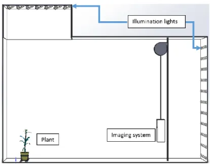
Figure 2.2 Setup of the hyperspectral imaging chamber
The imaging system consists of a push-broom type VNIR (visible and near infrared) scanner that collects images at wavelength bands between 546 nm and 1700 nm (Headwall Photonics, Fitchburg, MA, USA). One hyperspectral image cube consists of a total of 243 image bands, with a spectral sampling resolution of 4.7 nm per band. The scanning is done by a rotating mirror which sequentially exposes the
horizontal lines in an image from the top to the bottom. The resulting images have a spatial resolution of 420 rows by 320 columns. The images are taken against a white background, with lighting on the ceiling and on the wall behind the camera.
Figure 2.2 shows the setup of the hyperspectral imaging chamber. As shown in the figure, the chamber is illuminated by two banks of halogen lamps (35W, color temperature 2600 K), located on the ceiling above the plant and on the wall behind the imaging system.
2.5.2 Segmentation
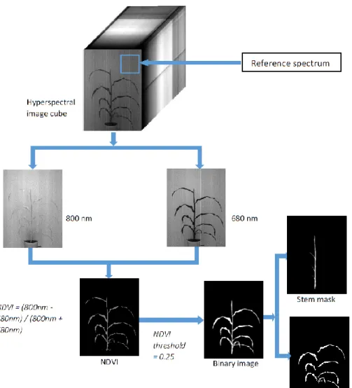
The segmentation of plant pixels in the hyperspectral images was achieved by making use of the rapid increase in reflectance of vegetation at the “red edge” of the electromagnetic spectrum. Red edge NDVI values are calculated by taking a
normalized difference between the reflectance at a near infrared band and a red band. Here, the NDVI values calculated for 680 nm (red band) and 800 nm (near infrared band) were found to separate the plant pixels well from the non-plant pixels in the hyperspectral images. A global threshold of 0.25 was used to get a binary mask from this image, where the higher values belonged to the plant pixels. This binary mask was then used for segmentation of each image bands in the
hyperspectral cube.
Stem and leaves were fractionated in the image by using the reflectance values at 1056 nm and 1146 nm. The ratio of pixel intensities at 1056 nm to the intensities at 1146 nm produced an image with the leaves and stem well separated. Using a global threshold value of 1.1, a binary mask to segment the stem was
obtained. This binary image was used with the mask for the whole plant to get the mask for the leaves. The stem section was manually divided into the top 1/3, the middle 1/3, and the bottom 1/3 of the length in order to have spectral data
corresponding to the samples collected from different plant sections. For images of plants that had a grain head on the day of sampling, the pixel intensities for the grain head were not included in the top section of the stem. The complete segmentation process is shown in Figure 2.3.
Since the spectral information extracted from the images was in the form of 8-bit pixel intensity values, noise present in the images was directly observable in the extracted spectra. Moreover, the spectra did not represent true reflectance values. In order to
convert to reflectance, the intensity values were divided by reference values extracted from the images. This was done by selecting a rectangular region in the image
background that did not contain the plant, and extracting “reference” spectra from the selected pixels. Once the reflectance spectra were obtained in the form of ratios, noise reduction was done by a moving average. This resulted in a dataset that contained a unique spectrum for each section of a plant.
2.5.3 Chemometric models
Partial least squares regression (PLSR) was the statistical technique used for developing models for the estimation of plant chemical properties from spectral data. PLSR is a generalized technique of multiple regression which is suited for spectral data because of its ability to perform well with data that contains highly correlated variables, and its robustness in the presence of noise. It is regarded as a standard in the field of chemometrics, and in case of vegetation, PLSR models built
with hyperspectral data outperform regression models based on traditional spectral indices (Atzberger, Guérif, Baret, & Werner, 2010; Wold, Sjöström, & Eriksson, 2001).
PLSR models were built using the spectral data collected from two methods: the spectral data collected from dried and ground biomass, and the spectral data extracted from the images. The spectral data from both sources were used to build models for all of the chemical properties: macronutrients (N, P, and K), NDF, and ADF. Since the data extracted from hyperspectral images had a smaller range of wavelengths and a lower spectral resolution, the spectral data of the dried biomass (obtained using a spectrometer) were resampled so that the model performance could be compared.
The scheme of leave one out cross validation was used for the determination of the optimum number of variables used in the PLSR models. The smallest RMSE value was taken as the criterion for the selection of this number. As measures of the
performance for the different models, RMSE values of cross validation, R2 values,
and ratio of performance to deviation (RPD) values were calculated. Leave-one-out scheme of cross validation was used since the number of samples was not large enough for separation into calibration and validation sets.
Pairwise score plots for the first three principal components were created for the spectral data to identify outliers and to observe underlying patterns in the data. No spectral outliers were observed.
CHAPTER 3
RESULTS AND DISCUSSION
3.1 SHOOT FRESH WEIGHT
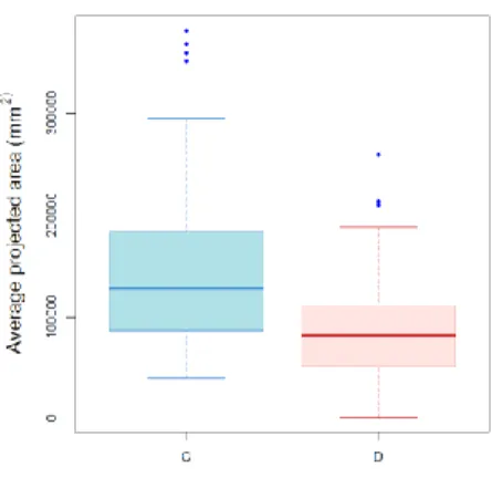
The values of the shoot fresh weight in gram are presented in the boxplots in Figure 3.1
(a).The separation is shown between the group subjected to drought stress (M = 106.91,
SD = 62.11), and the control group (M = 220.36, SD = 126.60). The difference in the mean fresh weights, displayed in figure 3.1 (a), was found to be significant according to
Welch’s two sample t-test (t(187.27) = 9.45, p < 2.2 x 10⁻⁶). Figure 3.1(b) shows the
boxplots for the area of plant pixels in the RGB images, averaged for the five side views. An analysis of variance indicates significant main effects of both the water treatment (F(1, 206) = 274.94, p < 0.0001), and the genotype (F(30,206) = 17.86, p < 0.0001). It also shows significant interaction effects, (F(29,206) = 5.36, p < 0.0001).
Figure 3.1. (a) Boxplots demonstrating the distribution of fresh shoot weights in the drought stressed group D and control group C (b) Distribution of the average area in square millimeters covered by plant pixels on the RGB images; the areas from five side view images have been averaged
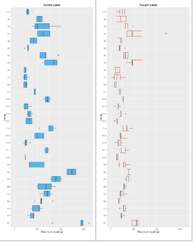
Figure 3.2. Boxplots demonstrating the distribution of fresh shoot weights in the drought stressed and control groups for each genotype in the experiment
In order to investigate the simple effects of the drought stress and genotype, boxplots showing distribution of data for different genotypes in both the control and drought groups are shown in Figure 3.2. The weights for plants from all of the sorghum lines are lower for the drought stressed plants, but variations can be observed in the effect of this treatment.
3.2 ESTIMATION OF FRESH SHOOT WEIGHT FROM RGB IMAGES
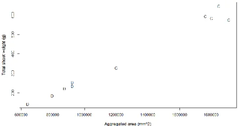
Figure 3.3 shows the correlation between aggregated area from plant images and the shoot fresh weight, r(276) = 0.91, p<0.0001. The plants that had a head at the time of imaging and sampling and the plants that did not have a head are represented by different symbols.
Figure 3.3. Correlation between total shoot fresh weight and the sum of area occupied by plant pixels in the five side view images.
The linear regression model has an R2 value of 0.83, and an RMSE value of 45.55. The distribution of points in the graph clearly indicates that the plants with a head and those without a head have different distributions. This can be attributed to the higher density of the grain heads, which means that the heads occupy a relatively smaller area in the image but constitute a disproportionately large fraction of the total shoot weight. The two groups can be seen separating to a greater extent as the weights increase, because the weights for the heavier plants with the grain head tend to be concentrated in the grain heads. As the heads increase in size, the weight per pixel ratio keeps increasing. For a sample of 65 plants, the gram per pixel values for head pixels had a mean and standard deviation of 0.0072 and 0.0031, respectively; whereas the gram per pixel values for non-head pixels had a mean and standard deviation of 0.0034 and 0.0008 respectively.
Figure 3.4. Correlation between total shoot fresh weight and the sum of area occupied by plant pixels for plants before head emergence
Figure 3.4shows the correlation between shoot fresh weight and total area for the plants
harvested before emergence of a head. The R2 value increases to 0.902, and the RMSE
value decreases to 37.36 g. The four isolated points on the upper right were investigated to detect the cause of their extreme values. All four points were found to be from the line E1, and all four plants were control plants. The correlation diagram was drawn only for E1 plants to see if there were anomalies to be detected. Figure 3.5 shows the points for the plants from the line E1. The images for these specific plants were also reviewed, and no special difference was observed except for the fact that these were relatively bigger plants. Figure 3.6 also shows the correlation for plants with a grain head present at the time of harvest.
Figure 3.5. Correlation diagram for plants belonging to the line "E1" The plants in the control group are denoted by "C" whereas the plants in the drought group are denoted by "D"
Figure 3.6. Correlation between total shoot fresh weight and the sum of area occupied by plant pixels for plants with emerged head during sampling
In Figure 3.4, the points appear to follow a polynomial trend rather than a linear one. A quadratic model was built to observe if it would fit better with the data. The resulting quadratic model is displayed in Figure 3.7. As expected, the quadratic model appears to
fit the data better. It also has a higher R2 value, and RMSE is reduced. This also removes
the concern of the negative intercept present in the linear model. This model was selected for the estimation of shoot fresh weight in analyzing the time series data. The total
Figure 3.7. Shoot fresh weight and aggregated area used to fit a quadratic model
3.3 ESTIMATION OF SHOOT DRY WEIGHT
A quadratic model was similarly found to fit satisfactorily with the dry shoot weights. Figure 3.8 shows the quadratic model for the estimation of dry weights. Again, the images of plants before the emergence of grain head were used.
3.4 RELATIVE GROWTH RATE ANALYSIS
For the available relative growth rates between DAP 49 and 70, analysis of variance was done for each day with the treatment and variety as the independent variables. The DAPs used for the analysis were 53, 55, 58, 60, 62, 64, 66, and 68. The data for day 51 was available, but the factorial ANOVA could not be carried out because the drought treatment was started on 53 DAP. On DAP 51, one-way ANOVA was conducted and RGR was found to be significantly different among varieties, F(29,186) = 1.63, p = 0.03.
Figure 3.8. Shoot dry weight and aggregated area used to fit a quadratic model
On 53 DAP, the treatment effect is still insignificant, F(1,166) = 0.02, p = 0.88. This was to be expected because the effect of the drought stress was not yet apparent. A study of the watering data confirms the fact that pot weights for plants under drought treatment was not noticeably lowered until at least two watering cycles. Variety was found to have
a significant effect for DAP 53, F(29,166) = 4.24, p = 1.4x10⁻⁹).
Significant effect of treatment is seen on RGR starting on 55 DAP, F(1,178) = 7.02, p = 0.008. This is the point at which the pots with plants subjected to drought would have lost enough water through evapotranspiration such that the plants were under stress. This is further supported by the fact that the treatment effect becomes highly significant with time. The F statistics and the p values yielded for DAP 58 to 68 are shown in Table 3.1.
Table 3.1 Results of the factorial ANOVA for RGR values for control and drought-stressed groups, from DAP 58 to 68
DAP Treatment Variety 58 F(1,177) = 18.16, p =3.3x10⁻⁵ F(29,177) = 1.56, p = 0.04 60 F(1,180) = 79.71, p = 4.9x10⁻¹⁶ F(29,180) = 4.23, p = 9.1x10⁻¹⁰ 62 F(1,169) = 135.32, p < 2.2x10⁻¹⁶ F(29,169) = 5.16, p = 3.1x10⁻¹² 64 F(1,164) = 191.12, p < 2.2x10⁻¹⁶ F(29,164) = 4.09, p = 3.7x10⁻⁹ 66 F(1,172) = 175.92, p < 2.2x10⁻¹⁶ F(29,172) = 3.75, p = 3.1x10⁻⁸ 68 F(1,163) = 110.92, p < 2.2x10⁻¹⁶ F(29,163) = 2.09, p = 0.002
Figure 3.9 shows the plots for relative growth rates of plants subjected to drought treatment and the control between DAP 51 to DAP 68. The plot marked “C” represents the average of values in the control group whereas the plot marked “D” represents the average in the drought group.
The plots show a gradual change in the relationship between the growth rates for the two groups. The difference between the two groups increases as the effect of drought becomes more pronounced with time. This information can also be derived from table 3.1 where the p-value rapidly decreases implying an increasing difference between the mean of two groups.
The fluctuating values of RGR can also be observed in Figure 3.9, for plants under drought stress as well as for the control group. For instance, the RGR values for 62 DAP noticeably increase to higher values before they decrease again on subsequent days. Since the fluctuation occurs for all of the plants on a particular day, it can be concluded that this change in RGR values is driven by environmental conditions.
The effect of genotype is found to be significant on all of the days included in the analysis. This trend was also verified by the growth rate of the different genotypes observed in the greenhouse as well as in the collected images. The biomass accumulation rate, as well as the final weight of the plants during harvest varied greatly across different genotypes.
3.5 CLIMATE DATA
The data on temperature, relative humidity, and radiation intensity recorded in the greenhouse during the days of growth were plotted to see if extreme changes in environmental conditions had occurred. Figure 3.10 shows the change in these values with time. The values for daytime temperature and relative humidity approach a peak between DAP 58 and DAP 64. During this period, the growth rates for plants under drought stress as well as for the plants in the control group are noticeably in an increasing trend as seen in Figure 3.9.
Figure 3.9 Relative growth rates for the control and drought groups from DAP 58 to DAP 68. "C" stands for the control group and "D" stands for the drought group; error bars show a 95% confidence interval for the mean
Figure 3.10. Changes in greenhouse environmental factors during the analysis period.
3.6 WATER USE EFFICIENCY
Water use efficiency (WUE) was calculated for the days between DAP 51 and 68. The WUE values were found to be greatly fluctuating not only with changes in genotype or presence of drought, but also with time, possibly due to the environmental effects.
In order to investigate whether a pattern in WUE values could be detected with respect to genotype, 58 DAP was chosen. The plant genotype had a significant effect on WUE value on this day, ((F(29,178) = 2.1044, p = 0.0017), whereas the effect of drought stress
was not found to be significant, (F(1,178) = 1.1554, p = 0.2838). Figure 3.11shows the
boxplots of WUE values for the plants under drought stress and control groups for 58 DAP.
Figure 3.11. Boxplots showing the distribution of WUE values in the control and drought groups for day 58.
Figure 3.12 shows the boxplots of the WUE values separated by drought and control, and also by the genotype. A few preliminary observations are possible if we look at the differences existing in the distributions of WUE values for the plants from the same line. For example, the line E3 appears to have higher values of WUE for plants subjected to drought compared to the values for plants in the control group. The results of a Welch’s two sample t-test shows marginally significant effect of the drought stress (t(3.91) = 2.62, p = 0.060). The line E8 has distributions tending towards higher values for plants in the control group compared to the plants under drought stress. The results of the t-test show an insignificant difference between the two groups, (t(3.68) = 1.36, p = 0.251). The variation in WUE values is clearly affected by both the genotype and the presence of drought stress.
Figure 3.12. Boxplots showing the difference in WUE values by treatment and variety for DAP 58
3.7 RANKING OF GENOTYPES
Figure 3.13 shows barplots of RGR and WUE ratios for the different genotypes. The RGR ratio is calculated by dividing the RGR values for drought stressed plants by the RGR values for plants in the control group. The same procedure is followed for calculating the WUE ratio.
Figure 3.13. Barplots showing the ratio of RGR and WUE values for different genotypes; the values for drought plants are divided by the values for control plants to derive the ratios
Since the principal trait of interest is the biomass yield of the sorghum plants, similar ranking was done for the total fresh weight of the plants at the time of harvest. Figure 3.14 shows the barplots for the average fresh weights by genotype.
Figure 3.14 Barplot showing the average biomass yield by genotype
We do not see a direct correlation in the values of RGR and WUE ratios and the total biomass yield. This is to be expected since the ratios can be high for genotypes that are better at adapting to drought, but may still be unproductive in terms of biomass.
3.8 CHEMICAL ANALYSIS
The concentrations of macronutrients (N, P, and K), and the NDF and ADF values obtained from different plant sections are shown in Figure 3.15. N, P, and K are in percentage units, whereas NDF and ADF values are the ratios of the NDF and ADF weight to the total dried biomass weight. The difference in the nutrient concentration among different plant tissues as well as the difference in cell wall composition can be clearly observed in the boxplots. Groups labeled with different alphabets are significantly different according to the Tukey Honest Significant Difference test (at significance level 0.05).
The plots for all the chemical properties show the leaf samples are different from the stem samples. Variation among the different stem sections can also be seen in some chemical properties such as potassium. This variation in chemical concentration among plant sections is one of the rationales for the use of two dimensional plant images in chemical phenotyping.
3.9 PLSR MODELING WITH SPECTROMETER DATA
The pairwise score plots of the first three principal components of the spectra obtained by scanning the dried and ground samples with the ASD spectrometer are shown in Figure 3.16. The plots show that the leaf spectra are well separated from the stem spectra in plots of PC1 vs. PC2 and PC1 vs. PC3.
The stem sections, however, do not seem to have obvious separation in these PC spaces. This is largely in agreement with the observation of chemical data, where the
difference between the leaves and the stem sections was found to be more prominent than that among different stem sections.
Figure 3.15. Boxplots showing the distribution of chemical properties in different plant sections. Plots marked with different alphabet labels are significantly different according to Tukey Honest Significant Difference test at significance level 0.05.
The results of the PLSR modeling using the spectrometer data are shown in Figure 3.17 and Table 3.2. The modeling was done after removing the spectral bands corresponding to the first 100 wavelength bands, where the signal was found to be noisy. Thus, the effective spectral range for these models was from 450 to 2500 nm. Figure 3.17 shows the coefficients of the regression models built for each chemical properties.
The four plots (corresponding to N, P, K, and NDF) show a distribution of heavily weighed variables throughout the wavelength range, whereas the plot of the coefficients for the ADF model peaks near the lower end and tends to zero for most of the wavelength range. Since this implies that most of the variables in the ADF model are weighed
extremely low, we can assume that the model built for ADF will possibly be less robust. This is verified later by the results presented in Table 3.2.
Figure 3.16. Score plots of the first three principal components. The samples from different sections (leaf, bottom, mid, and top) of the plants are shown with different legends.
Table 3.2. Cross validation results for N, P, K, NDF, and ADF with PLSR modeling using spectra from the ASD spectrometer.
Chemical properties No. of samples Model size R2 RMSEP RPD Nitrogen 116 116 0.89 0.28 2.98 Phosphorus 115 13 0.49 0.09 1.53 Potassium 116 13 0.61 0.70 1.60 NDF 126 11 0.62 0.05 1.62 ADF 52 1 0.13 0.09 1.08
From Table 3.2, we can see that the model for nitrogen performed the best with the R2
value of 0.89. Potassium, NDF, and phosphorus models were found to be fairly accurate. The RPD value is commonly used as a criterion for model performance. RPD values between 1.5 and 2 are considered to be of fair quality for quantitative prediction. The
model with the RPD value below 1.4 (or a corresponding R2 value less than 0.5) is not
suitable for quantitative prediction. Here, the model for ADF is found to be inadequate according to this criterion. However, models unsuitable for quantitative prediction can still be useful for qualitative screening, and their performance can be improved if potential areas of improvement are identified.
Figure 3.17. Regression coefficients of the PLSR models built for prediction of chemical concentrations using the spectral data from the ASD spectrometer.
A review of recent development in NIR spectroscopy for plant mineral characterization was presented by van Maarschalkerweerd & Husted ( 2015). They presented a summary of the results from various studies involving Vis-NIR spectroscopy of plant material. Table 3.3 is a condensed form of this table where the studies involved have all used dried, ground material. The wavelength range used in the study, the plant material, and the RPD values of the models formed by using RMSEP (or RMSECV) are shown in the table.
Across the studies, the models for nitrogen are found to be the most accurate, although the accuracy greatly varies among the different studies. This is in agreement with our results. The variation of the model accuracy among different species is to be expected because the response of the plant material to the electromagnetic spectrum depends on a large number of factors that may not be directly related to the concentration of a particular nutrient. An element may be present in a compound that does not respond vibrationally to the incoming radiation; but since the element will still be detected in the laboratory analysis, this can decrease the accuracy of the model. The presence of biotic or abiotic stress can also affect the interaction of molecules with the incoming light. The presence of a large number of sorghum genotypes in this study led to a great variation in the concentration of the nutrients, but the underlying changes in the plant physiology and structure could act against the effectiveness of the models. The prediction plots of the
Table 3.3 Summary of studies on Vis-NIR calibration for the estimation of nutrient concentrations using dried and ground biomass.
Author Wavelength range
Plant material RPD N P K Agnew, Park, Mayne,
& Laidlaw, 2004
400–2500 Dry, ground
ryegrass
6.5
Chen et al., 2002 400-2500 Dry, ground
sugarcane leaves
1.7 Cozzolino & Moron,
2004
400-2500 Dry, ground
Lucerne, and clover de Aldana, Criado,
Ciudad, & Corona, 1995
1100-2500 Dry, ground grasses 3.9 1.5 1.8
Huang, Han, Yang, & Liu, 2009
400-2500 Dry, ground or cut
wheat and rice straw
1.7 (cut) 2.6 (milled) Liao, Wu, Chen, Guo,
& Shi, 2012
1100-2500 Dry, ground tree
leaves
2.5 1.4 1.2
Petisco et al., 2005 1100-2500 Dry, ground tree
leaves
4.3 2.3
Petisco et al., 2008 1100-2500 Dry, ground tree
leaves
2.4 Ward, Nielsen, &
Møller, 2011
Figure 3.18. Plots showing the predicted chemical concentration against lab measured values for N, P, K, NDF, and ADF.