Two fast integrators for the Galactic tide effects in the Oort Cloud
S. Breiter,
1M. Fouchard,
2,3R. Ratajczak
1and W. Borczyk
11Astronomical Observatory of A. Mickiewicz University, Stoneczna 36, Pozna´n 60-286, Poland 2INAF–IASF Roma, Via del Fosso del Cavaliere 100, 00133 Roma, Italy
3IMCCE/SYRTE, Observatoire de Paris, 77 av. Denfer-Rochereau, 75014 Paris, France
Accepted 2007 February 21. Received 2007 February 15; in original form 2006 July 10
A B S T R A C T
Two fast and reliable numerical integrators for the motion of the Oort Cloud comets in the Galactic tidal potential are presented. Both integrators are constructed as Hamiltonian splitting methods. The first integrator is based upon the canonical Hamiltonian equations split into the Keplerian part and a time-dependent perturbation. The system is regularized by the application of the Kuustanheimo–Stiefel variables. The composition rule of Laskar and Robutel with a symplectic corrector is applied. The second integrator is based on the approximate, averaged Hamiltonian. Non-canonical Lie–Poisson bracket is applied allowing the use of non-singular vectorial elements. Both methods prove superior when compared to their previously published counterparts.
Key words: methods: analytical – methods: numerical – celestial mechanics – comets: general – Oort Cloud.
1 I N T R O D U C T I O N
Galactic tides are one of the essential factors determining the evo-lution of cometary orbits in the Oort Cloud. In the absence of an analytical solution describing the motion of comets under the ac-tion of the complete Galactic tide potential, numerical integraac-tion remains the main path to the understanding of the Oort Cloud dy-namics between sporadic events like stellar encounters. Gaining knowledge of a dynamical system through numerical integration is a fairly time-consuming process: huge samples of orbits spanning the whole phase space have to be simulated. In recent years, a num-ber of papers were published proposing new tools that may replace a slow, general purpose integrator of high order. Brasser (2001) vaguely reported the application of a presumably fast symplectic integrator of Mikkola. Fast mappings were proposed in Fouchard (2004); Fouchard et al. (2005, 2006), where a detailed accuracy and performance tests can also be found. Another line of improve-ment was proposed by Breiter & Ratajczak (2005) (see also Breiter & Ratajczak 2006) who suggested the use of non-canonical Hamiltonian formalism. Their Lie–Poisson integrator was designed for axially symmetric Galactic disc perturbations.
In the present paper, we report two complementary integrators that extend and improve the methods presented in Fouchard (2004); Fouchard et al. (2005, 2006) and Breiter & Ratajczak (2005). Both methods belong to a class of Hamiltonian splitting methods: one of them integrates the exact equations of motion, and the other one handles a first-order normalized (averaged) system.
E-mail: [email protected] (SB); [email protected] (MF); astromek @amu.edu.pl (RR); [email protected] (WB)
Using the terminology of McLachlan & Quispel (2002), a split-ting method consists of three elements: partitioning the right-hand sides into a sum few vector fields, solving the equations of motion induced by each vector field,1and combining these solutions to yield an integrator. The last element (to a large extent independent of the first two) is usually referred to as ‘composition’. Thus a splitting method for a particular system necessarily involves some compo-sition method responsible for its local truncation error, but it is the partitioning that determines additional properties of the integrator. Namely, if the system is Hamiltonian and each vector field remains Hamiltonian, the integrator will conserve the symplectic or Poisson structure of the flow regardless of the composition method applied. As a side effect, the Hamiltonian function has no secular error apart from round-off effects.
Sometimes a splitting method can be improved by adding an extra stage known as a corrector. Derived from some combination of the partitioned right-hand side terms, it does not increase the power of step size in the local truncation error estimate, yet it may effectively decrease the local error by introducing an extra factor independent of the step size. For example, the symplectic correctors may diminish the error of a Hamiltonian function in the situation when one of the terms in a partitioned Hamiltonian is much smaller than the other (Wisdom, Holman & Touma 1996; Laskar & Robutel 2001; McLachlan & Quispel 2002). Our first integrator (LARKS – after the names of Laskar, Robutel, Kuustanheimo and Stiefel), described in Section 2, employs the composition method and the symplectic corrector of Laskar & Robutel (2001) in the framework
1The solutions can be either exact or approximate, but we assume only the former case in the present paper.
of the Kuustanheimo–Stiefel (KS) variables. To a large extent, it can be considered as a direct descendant of the T-REX method of Breiter (1998).
The second method, presented in Section 3, integrates first-order normalized equations of motion that no longer depend on the mean anomaly. They are derived from a Hamiltonian function with a non-canonical Lie–Poisson bracket. Thanks to the use of ‘vectorial ele-ments’ (dimensionless Laplace vector and angular momentum vec-tor), no singularities are met regardless of orbital eccentricity and inclination. This approach already proved fruitful for the Galactic disc problem (Breiter & Ratajczak 2005, 2006). The method will be referred to as Lie-Poisson with Vectorial elements (LPV). Unlike LARKS, the integrator is based on the partition of the Hamiltonian into three terms of similar magnitude, thus the application of a cor-rector is neither easy nor advantageous, so only usual symmetric composition methods are applied.
Both integrators are also supplied with algorithms that allow the propagation of the associated variational equations. This feature is of great importance for distinguishing regular and chaotic orbits, be-cause many of the chaos detectors rely on checking the exponential growth of the variations vector.
Section 4 presents performance tests and resolves some technical questions related to the step size choice.
2 R E G U L A R I Z E D S Y M P L E C T I C I N T E G R AT O R
2.1 Equations of motion
2.1.1 Hamiltonian in Cartesian variables
Let us consider the motion of a comet in a right-handed heliocen-tric reference frameOxyz. The fundamental planeOxyis parallel to the Galactic disc and the axisOzpoints towards the North Galactic Pole. If we fix the orientation of theOxaxis such that at the initial epoch t= 0 it is directed to the Galactic Centre, we will obtain an explicitly time-dependent problem of the heliocentric Keplerian motion perturbed by the tidal force of the Galaxy. The time depen-dence comes from the orbital motion of the Sun around the Galactic Centre. Assuming the circular orbit of the Sun, we can represent the heliocentric motion of the Galactic Centre as a uniform rotation with the angular rate0<0. Thus, similar to Fouchard (2004), we can assume the Hamiltonian function
H=H0+H1 (1) H0= 1 2 X2+Y2+Z2−μ r, (2) H1= 1 2 G1x2 1+G2y21+G3z2 , (3)
wherex1andy1 are the projections of a comet radius vectorr = (x,y, z)T on to the direction towards the Galactic Centre and its perpendicular
x1=xcos0t+ysin0t,
y1= −xsin0t+ycos0t. (4) The uppercaseX,YandZstand for the momenta canonically con-jugate to the respective lowercase coordinates.
The physical constants appearing in the Hamiltonian involve the heliocentric gravitational parameterμ=GMand parametersGi
related to the Oort constants of our Galaxy. Following Levison,
Dones & Duncan (2001), we adopt G2= −G1=7.0706×10⁻¹⁶yr−2, G3=5.6530×10⁻¹⁵yr−2, 0= − √ G2. (5)
Introducing the first of equations (5) explicitly, we can rewriteH1 as H1(x,y,z,t)= 1 2G2 (y2−x2)C−2x y S+1 2G3z 2, (6) where C=cos (20t), S=sin (20t). (7) It is well known that in cometary problems one cannot expect to meet moderate eccentricities of orbits; some kind of regularization will become unavoidable if a fixed step integrator is to be applied. One of the standard regularizing tools, successfully tested in celes-tial mechanics over decades, is the application of the so-called KS transformation that turns a Kepler problem into a harmonic oscilla-tor at the expense of increasing the number of degrees of freedom (Stiefel & Scheifele 1971). Out of numerous ways of settling the KS variables in the canonical formalism, we choose the approach of Deprit, Elipe & Ferrer (1994), warning readers that the labelling of variables may differ from the one commonly repeated after the Stiefel and Scheifele textbook.
2.1.2 KS variables
Leaving apart the in-depth quaternion interpretation of the KS trans-formation given by Deprit et al. (1994), we restrict ourselves to pro-viding the basic set of transformation formulae, treating the KS vari-ables as a formal column vector. In the phase space of the KS coordi-nates,u=(u0,u1,u2,u3)Tand KS momentaU=(U0,U1,U2,U3)T, the former are defined by means of the inverse transformation x =u2 0+u21−u22−u23 /α, y=2 (u1u2+u0u3)/α, z =2 (u1u3−u0u2)/α, (8)
whereαis an arbitrary parameter with a dimension of length. A dimension raising transformation cannot be bijective, so the inverse of (8) is to some extent arbitrary. Following Deprit et al. (1994), we adopt u= α 2 (r+x) (0,r+x, y,z) T, (9) forx0, and u= α 2 (r−x) (−z, y,r−x,0) T, (10)
otherwise. A remarkable property of this transformation is that the distancerbecomes a quadratic function ofui, namely
r=x2+y2+z2= u 2 0+u21+u22+u23 α = u2 α. (11)
The momenta conjugate touare defined as
U= α2 ⎛ ⎜ ⎜ ⎜ ⎝ u0X+u3Y−u2Z u1X+u2Y+u3Z −u2X+u1Y−u0Z −u3X+u0Y+u1Z ⎞ ⎟ ⎟ ⎟ ⎠. (12) 377,
The inverse transformation, allowing the computation of R= (X,Y,Z)T, R= 1 2r ⎛ ⎜ ⎝ u0U0+u1U1−u2U2−u3U3 u3U0+u2U1+u1U2+u0U3
−u2U0+u3U1−u0U2+u1U3
⎞ ⎟
⎠, (13)
can be supplemented with the identity
u1U0−u0U1−u3U2+u2U3=0, (14) that may serve as one of the accuracy tests during numerical integration.
In order to achieve the regularization without leaving the canon-ical formalism, we have to change the independent variable fromt to a fictitious timesand consider the extended phase space of di-mension 10, with a new pair of conjugate variables (u∗,U∗). Thus in the extended set of canonical KS variables, the motion of a comet is governed by the Hamiltonian function
M= 4αu22 K0+U∗+K1=0, (15) whereK0andK1stand forH0andH1, respectively, expressed in terms of the extended KS variables set. The presented transformation is univalent, hence the respective Hamiltonians will have different functional forms, but equal values:H0=K0,H1=K1. Restricting the motion to the manifold ofM=0 is of fundamental importance to the canonical change of independent variable; in practical terms we achieve it by setting
U∗= −K0−K1, (16)
at the beginning of the numerical integration.2
Splitting the Hamiltonian functionMinto a sum of the principal termM0and a perturbationM1, we have
M0= 1
2U
2+(4U∗/α2)u2, (17) M1= 4αu22H1(x,y,z,t). (18) We find it convenient to maintain H1 as a function of Carte-sian coordinates and time, because the values ofx, y, z can be quickly computed from equations (8) and partial derivatives re-quired in next sections are simple enough to provide compact expressions: ∂r ∂u T = α2 ⎛ ⎜ ⎜ ⎝ u0 u3 −u2 u1 u2 u3 −u2 u1 −u0 −u3 u0 u1 ⎞ ⎟ ⎟ ⎠. (19)
Although nothing prohibitsu∗andtto differ by an additive constant, we do not profit from this freedom and so we will use the symbolt in most of instances instead of the formalu∗. In the next section, we provide equations of motion generated byM0andM1alone; the complete equations of motion can quickly be obtained by adding the respective right-hand sides.
2More details concerning this kind of Hamiltonian regularization can be found in Szebehely (1967), Stiefel & Scheifele (1971) and Mikkola & Wiegert (2002).
2.2 Canonical splitting method 2.2.1 Keplerian motion
The principal virtue of the KS variables consists in their ability of transforming the Kepler problem into a harmonic oscillator. Indeed, M0leads to the equations of motion
du ds = ∂M0 ∂U =U, (20) dU ds = − ∂M0 ∂u = −(8U ∗/α2)u, (21) dt ds = ∂M0 ∂U∗ =4u 2/α2, (22) dU∗ ds = − ∂M0 ∂t =0. (23)
Equations (20) and (21) define a four-dimensional oscillator with a frequency
ω=2
√
2U∗
α , (24)
and equation (23) indicates that the frequency is constant. Equa-tion (22) explains the meaning of the fictitious times: we can rewrite it as
ds dt =
α
4r. (25)
Thus, supposing that we study Keplerian motion on an ellipse with a semi-axisa, ds/dt equals to (α/4a) dE/d, where Eand are the eccentric and the mean anomaly, respectively. It means that apart from a multiplier, the fictitious time s behaves like eccentric anomaly, albeit the former is not an angle and can-not be treated ‘modulo period’. Thanks to the introduction of α, the fictitious time s has the dimension of time and if we assume
α= |2μ
U∗|, (26)
orbital periods in s and t will be equal in the elliptic motion. It should be noted, however, that the oscillator defined by M0 has the frequency ω = n/2 (where nis the mean motion), i.e. the Keplerian ellipse period in Cartesian coordinates is two times shorter than the KS oscillator’s period in t. This fact is a direct consequence of equations (8); by a simple analogy, the square of a 2π periodic sine function is only π periodic. Thus, select-ing the integration step, one has to bear in mind that one cy-cle of the KS oscillator maps on two revolutions in the Cartesian space.
ForU∗>0, the map0representing the solution of equations (20)–(23) can be directly quoted from Breiter (1998). Ifis the fictitious time-step, then
0,: ⎛ ⎜ ⎝ u U U∗ ⎞ ⎟ ⎠→ ⎛ ⎜ ⎝ ucosω+Uω−1sinω −uωsinω+Ucosω U∗ ⎞ ⎟ ⎠. (27) Additionally, ifv=0,uandV=0,Uare the final values of
variables, 0,: t→t+2α2 u2+U2 ω2 +2u TU−vTV α2ω2 . (28)
One may easily check that the sumu2+U2ω−2is invariant under 0and it can be replaced byv2+V2ω−2in practical computations of the Kepler equation (28).
It may happen, however, thatU∗<0 and the motion is (at least temporarily) hyperbolic. A simple modification of0in that case amounts to taking
ω=2
√ −2U∗
α , (29)
and replacing equations (27) and (28) by
0,: ⎛ ⎜ ⎝ u U U∗ ⎞ ⎟ ⎠→ ⎛ ⎜ ⎝ ucoshω+Uω−1sinhω uωsinhω+Ucoshω U∗ ⎞ ⎟ ⎠, (30) and 0,: t→t+ 2α2 u2−U 2 ω2 −2u TU−vTV α2ω2 . (31)
Similarly to the elliptic case,u2−U2/ω2is invariant under 0. We do not provide the complete formulation forU∗ = 0, be-cause the probability of meeting this case is practically negligible. Actually, using the SBAB or SBABC composition methods (see Section 2.4), it is even not easy to create this case intentionally. We only observe that for a parabolic motion the selection rule ofα obviously cannot be based onU∗and then any choice, likeαequal to the osculating perihelion distance, is acceptable. The parabolic solution is easily derivable from equations (20)–(23) that lead to constantU,linear functions ofsforuand the quadratic function of sfort, whenU∗=0.
2.2.2 Galactic tide
HamiltonianM1has a nice property of being independent on mo-menta. Thus a half of the equations of motion have right-hand sides equal to zero, and the remaining right-hand sides are constant:
du ds = ∂M1 ∂U =0, (32) dt ds = ∂M1 ∂U∗ =0, (33) dU ds = − ∂M1 ∂u = −F(u,t), (34) dU∗ ds = − ∂M1 ∂t = − 4u2 α2 ∂H1 ∂t = −F ∗(u,t). (35)
Accordingly, all KS coordinates are constant, the physical timet does not flow, and the momenta are subjected to a linear ‘kick’
1,: ⎛ ⎜ ⎜ ⎜ ⎝ u t U U∗ ⎞ ⎟ ⎟ ⎟ ⎠→ ⎛ ⎜ ⎜ ⎜ ⎝ u t U−F(u,t) U∗−F∗(u,t) ⎞ ⎟ ⎟ ⎟ ⎠. (36)
Mixing Cartesian ad KS variables for the sake of brevity, we can representFandF∗as F= 8H1 α2 u+ 4u2 α2 ∂H1 ∂u (37) F∗= 4u 2 α2 0G2ξ3, (38) where ∂H1 ∂u = −G2ξ2 ∂x ∂u+G2ξ1 ∂y ∂u+G3z ∂z ∂u ξ1 = yC−x S, (39) ξ2= xC+y S, ξ3=(x2−y2)S−2x y C, (40)
∂x/∂uis the first column of the Jacobian matrix (19), and so on.
2.2.3 Symplectic corrector
One of the advantages offered by Laskar & Robutel (2001) inte-grators is a simple definition of a symplectic corrector – an extra stage that improves the accuracy in perturbed motion problems. The symplectic corrector is defined as a solution of equations of motion generated by
Mc= {{M0,M1},M1}, (41) where{,}is the canonical (or ‘symplectic’) Poisson bracket in the phase space spanned byu,t,U,U∗. Observing thatM0is quadratic inUand linear inU∗, we easily obtain
Mc(u,t)= 3 i=0 ∂M1 ∂ui 2 =F2. (42)
The general form of equations of motion derived fromMcis simple du ds = ∂Mc ∂U =0, (43) dt ds = ∂Mc ∂U∗ =0, (44) dUj ds = − ∂Mc ∂uj = −2 ∂F ∂uj ·F(u,t), (45) dU∗ ds = − ∂Mc ∂t = −2 ∂F ∂t ·F(u,t), (46) and their solution is elementary, resulting in
c,: ⎛ ⎜ ⎜ ⎜ ⎝ u t Uj U∗ ⎞ ⎟ ⎟ ⎟ ⎠→ ⎛ ⎜ ⎜ ⎜ ⎜ ⎝ u t Uj−2 ∂F ∂uj ·F U∗−2∂∂tF·F ⎞ ⎟ ⎟ ⎟ ⎟ ⎠. (47)
In spite of a formally simple form, equations (47) involve rather complicated expressions for the second derivatives ofM1, because
∂F ∂uj ·F(u,t)= 3 i=0 ∂2M1 ∂ui∂uj ∂M1 ∂ui , (48) ∂F ∂t ·F(u,t)= 3 i=0 ∂2M1 ∂ui∂t ∂M1 ∂ui . (49) 377,
The Hessian matrix ofM1can be represented as a sum ∂2M1 ∂u2 = 8 α2 H1I4+u ∂H1 ∂u T +∂H1 ∂u u T + u2 2 ∂2H1 ∂u2 , (50)
whereI4is a 4×4 unit matrix, andxyTstands for the tensor product with components [xyT]
i j =xiyj. The Hessian ofH1is composed
of two matrices ∂2H1 ∂u2 = 2 α (G+A). (51) The matrixGis G= ⎛ ⎜ ⎜ ⎜ ⎜ ⎝ −G2ξ2 0 −G3z G2ξ1 0 −G2ξ2 G2ξ1 G3z −G3z G2ξ1 G2ξ2 0 G2ξ1 G3z 0 G2ξ2 ⎞ ⎟ ⎟ ⎟ ⎟ ⎠. (52)
The matrixAis symmetric, so only 10 of its elements have to be specified; using explicitly the KS coordinates, we obtain
a11 =G3u2 2−G2 u2 0−u23 C+2u0u3S, a22 =G3u2 3−G2 u2 1−u22 C+2u1u2S, a33 =G3u20+G2 u2 1−u22 C+2u1u2S , a44 =G3u21+G2 u2 0−u23 C+2u0u3S , a12 = −G3u2u3 −G2[(u0u1−u2u3)C+(u0u2+u1u3)S], a13 =G3u0u2
+G2[(u0u2+u1u3)C−(u0u1−u2u3)S], a14 = −G3u1u2+ G2 2u0u3C− u2 0−u23 S, a23 = −G3u0u3+ G22u1u2C−u2
1−u22 S, a24 =G3u1u3 +G2[(u0u2+u1u3)C−(u0u1−u2u3)S], a34 = −G3u0u1 +G2[(u0u1−u2u3)C+(u0u2+u1u3)S]. (53)
Partial derivatives required in (49) are simpler:
∂2M1 ∂u∂t = 80G2 α2 ξ3u−u2H , (54) where H= ⎛ ⎜ ⎜ ⎜ ⎝ (u3x+u0y)C+(u3y−u0x)S (u2x+u1y)C+(u2y−u1x)S (u1x−u2y)C+(u1y+u2x)S (u0x−u3y)C+(u0y+u3x)S ⎞ ⎟ ⎟ ⎟ ⎠. (55)
At the first glimpse, one may hesitate if the cost of computing the corrector is worth the gain in accuracy from the point of view of the computation time. The doubts, however, will be quickly dismissed when the tangent map is to be attached to the integrator. The next section shows that the second derivatives presented above are also required for the tangent map, hence in that case the corrector is actually evaluated almost at no cost.
2.3 Tangent maps
Considering the sensitivity of motion to the initial conditions, either for the chaos test or for the differential correction of orbits, one has to know the evolution of the tangent vectorδdescribing an in-finitesimal displacement with respect to the fiducial trajectory in the phase space. Althoughδis formally infinitesimal, it obeys homo-geneous linear equations of motion (variational equations), which means that we can multiply it by an arbitrary constant and use the initial value ofδnormalized toδ=1. From the formal point of view, we should integrate the linear system of variational equations derived from the equations of motion generated byM; but this is by no means a simple way – far more complicated than taking the shortcut indicated by Mikkola & Innanen (1999) that amounts to linearizing the maps0and1. Thus we provide expressions of ‘tangent maps’D0 andD1that serve to propagate the tangent vectorδsimultaneously with the integration ofu,U,tandU∗. As a matter of fact, we should also provide a tangent mapDc, but computing third derivatives ofMdoes not seem attractive and we cut the Gordian knot by neglecting the corrector’s influence onδ.
2.3.1 Keplerian tangent map
Differentiating equations (27), (28) and their hyperbolic counter-parts, we obtain the tangent mapD0as the propagation rules for the tangent vectorδ. The initial values ofδwill be labelledδu, δU, δt andδU∗; the values after the fictitious time-stepwill be referred to asδv, δV, δtandδV∗. ThusδV∗=δU∗, and
δv=(δu)c+(δU)sω +(δωω) V−Us ω , (56) δV= ∓(δu)ωs+(δU)c∓(δω) (ωv+us), (57) δt=(δt)+ 4α2 u·(δu)±U·(δU) ω2 ∓ (δω) ω3 U 2 ±α22ω2[(δu)·U+u·(δU)−(δv)·V−v·(δV)] ∓4(α2δωω3)(u·U−v·V), (58) δω= ±4 (δU∗) α2ω . (59)
IfU∗>0, the upper signs should be taken in the above equations ands=sinω ,c=cosω . In the opposite case,s=sinhω
,c=coshω , and the lower signs are to be adopted.
2.3.2 Tidal tangent map
Differentiating the galactic tide map (36), we obtain formally simple expressions of the tangent mapD1
D1,: ⎛ ⎜ ⎜ ⎜ ⎝ δu δt δU δU∗ ⎞ ⎟ ⎟ ⎟ ⎠→ ⎛ ⎜ ⎜ ⎜ ⎝ δu δt δU−P δU∗−P∗ ⎞ ⎟ ⎟ ⎟ ⎠, (60)
where P= ∂F ∂u (δu)+(δt)∂F ∂t = ∂2M1 ∂u2 (δu)+(δt) ∂2M1 ∂u∂t , (61) P∗= ∂F∗ ∂u (δu)+(δt)∂F ∗ ∂t = ∂2M1 ∂u∂t (δu)+(δt) ∂2M1 ∂t2 . (62)
Most of the derivatives required for this tangent map can be found in Section 2.2.3, except for
∂2M1 ∂t2 = 8r α G220 (x2−y2)C+2x y S. (63)
2.3.3 Initial conditions for the tangent map
Choosing an appropriate initial direction of the variation vector is important; most of all, one should avoid the direction ofδparallel to the right-hand sides of equations of motion, because it leads to underestimated values of the maximum Lyapunov exponent and related chaos indicators (Barrio 2005). An optimum choice of initial δ is orthogonal to the flow. For the LARKS integrator, we have adopted a simplified approach, setting the variations orthogonal to the Keplerian flow, i.e.
δu= −U=8α−2U∗u, δU=u=U, δt= −(U∗)=0, δU∗=t=4α−2u2. (64) 2.4 Laskar–Robutel integrators
The composition methods of Laskar & Robutel (2001) differ from usual recipes, because regardless of the number of ‘stages’ involved in one step, they all remain second-order integrators according to the formal estimates (in this context the term ‘high order’ used by Laskar and Robutel is a bit misleading). However, if the Hamiltonian has been split into a leading term and a perturbation having a small parameter ε as a factor, the truncation error of the integrator is max (ε2h3,εhm) wheremis the number of stages involved in one
step. The second term of this sum is similar to classical composition methods errors, and the first can be quite small for weakly perturbed problems. At the expense of theε2h3term in the error estimate, the authors were able to avoid backward stages that degrade numerical properties of usual composition methods. The use of a corrector improves the integrator by reducing the truncation error: its first term drops toε2h5. Following the recommendation of Laskar & Robutel (2001), we have adopted their SBABC3 method as the optimum choice. In this case a single step of LARKS with the step sizehcan be written as h =c,q◦1,d1◦0,c2◦1,d2◦0,c3◦ ◦1,d2◦0,c2◦1,d1◦c,q, (65) where d1=h/12, d2=(5/12)h, c2=(1/2−√5/10)h, c3=h/√5, q= −h3(13−5√5)/288. (66)
However, this choice has not been made without numerical tests involving other composition rules with and without correctors. The results of our tests are given in Section 4.
The tangent mapDhis constructed similarly, but we have
de-cided to skip the correction part. There is no need to struggle for a high accuracy of variations vector as far as we are interested only in detecting its exponential growth. Thus
Dh = D1,d1◦D0,c2◦D1,d2◦D0,c3◦
◦D1,d2◦D0,c2◦D1,d1. (67)
3 L I E – P O I S S O N I N T E G R AT O R F O R T H E AV E R AG E D S Y S T E M
3.1 Equations of motion
The integrator presented in the previous section solves the equations of motion in the fixed reference frame, where the radial component of the Galactic tide is explicitly time-dependent. Our second method can be more conveniently discussed in a rotating heliocentric refer-ence frameOx1y1z. TheOx1y1plane remains parallel to the Galactic disc, but this timeOx1axis is directed towards the Galactic Centre hence the frame rotates around theOzaxis with the angular rate0. If we assume the right-handedOx1y1zsystem of axes and the axis Ozremains directed towards the North Galactic Pole, the rotation is clockwise, which implies0<0. The Hamiltonian function for a comet subjected to the Galactic tide in the rotating frame is given by H=H0+H1, (68) H0= 1 2 X2 1+Y12+Z2 − μ x2 1 +y12+z2 1 2 , (69) H1=0(y1X1−x1Y1)+ 1 2 G2y2 1−x12 +G3z2. (70) The first-order normalization ofHwith respect toH0is equivalent to averaging with respect to the mean anomalyand leads to the new Hamiltonian H∗=H∗ 0+H∗1, (71) H∗ 0= − μ 2a, (72) H∗ 1= 1 2π 2π 0 H1d, (73)
where the elliptic Keplerian motion is assumed to evaluate the quadrature in (73). The averaged HamiltonianH∗1attains the sim-plest form if expressed in terms of the Laplace vectoreand a scaled
angular momentum vectorh. Their components are related to the Keplerian orbit elements
e≡ ⎛ ⎜ ⎝ e1 e2 e3 ⎞ ⎟ ⎠=e
cosωcos−csinωsin cosωsin+csinωcos
s sinω , (74) h≡ ⎛ ⎜ ⎝ h1 h2 h3 ⎞ ⎟ ⎠=1−e2 s sin −s cos c , (75)
whereeis the eccentricity,s= sinI,c= cosI are the sine and cosine of the inclination,ωis the argument of perihelion and stands for the longitude of the ascending node with respect to the Galactic Centre. Recalling that in the rotating frame momentaX1 andY1 are not equal to velocities ˙x1 and ˙y1 (the fact that can be immediately deduced from the canonical equations ˙x1 =∂H/∂X1 and ˙y1 =∂H/∂Y1), we assume that the usual transformation rules between Keplerian elements and position/velocity are used with the velocities directly substituted by the momenta. With this approach the Keplerian motion in the rotating frame is described by means of orbital elements that are all constant except forwhich reflects the frame rotation ( ˙= −0).
Using the ‘vectorial elements’hande, and lettingnto stand for
n=
μ
a3, (76)
we obtain [Correction added after online publication 2007 April 13: in the first line of equation (77), a redundant pair of right square brackets appeared after1
4 and have been removed.] H∗ 1 = −0n a2h3+ 1 4a 2G25e2 2−5e 2 1−h 2 2+h 2 1 + +G31−e2+5e2 3−h23 . (77)
Strictly speaking, the HamiltonianH∗generates the motion of the mean variables in the linear approximation. Thus, using the solution generated byH∗we neglect short-period perturbations depending onthat are proportional to the small parameter≈H1/H0, and we commit an error of the order of2in the evolution of the mean elements. The influence of this approximation will be discussed later; meanwhile we accept the first-order correct, mean elements that liberate us from discussing the mean anomalyand lead to the constant value of the mean semimajor axisa. As a consequence, we can drop constant terms fromH∗and change the independent variable from timettoτ1, such that
dτ1 dt =
G3
n. (78)
Using the usual approximation0= −
√ G2, we introduce a dimen-sionless parameter ν= 20 G3 = G2 G3, (79)
and thus we replaceH∗by [Correction added after online publication 2007 April 13: in the first line of equation (80),h2
1+was omitted after the first 1
4 and an extra+symbol appeared at the end of the line.] H=n a2 5 4e 2 3+ 1 4h 2 1+ 1 4h 2 2 +ν −5 4e 2 1+ 5 4e 2 2+ 1 4h 2 1− 1 4h 2 2−n−01h3 . (80)
The vectorial elements can be used to create a Lie–Poisson bracket (f;g)≡ ∂f ∂v T J(v)∂g ∂v, (81)
with the structure matrix J(v)= ˆ h eˆ ˆ e hˆ . (82)
The ‘hat map’ of any vectorx=(x1,x2,x3)Tis defined as ˆ x= 0 −x3 x2 x3 0 −x1 −x2 x1 0 . (83)
This matrix is known as the vector product matrix, because ˆ
xy=x×y. (84)
Using the Lie–Poisson bracket (81), we can write equations of mo-tion for the vectorial elements
v=(h1,h2,h3,e1,e2,e3)T, (85)
in the non-canonical Hamiltonian form
v=(v;K), (86)
where derivatives with respect toτ1 are marked by the ‘prime’ symbol and the scaled Hamiltonian
K= −H
n a2. (87)
Writing equations (86) explicitly, we obtain h1= −5 2(1−ν)e2e3+ 1−ν 2 h2h3+ nν 0 h2, (88) h2= 5 2(1+ν)e1e3− 1+ν 2 h1h3− nν 0 h1, (89) h3=ν(h1h2−5e1e2), (90) e1= −4+ν 2 h2e3+ 5 2νh3e2+ nν 0 e2, (91) e2= 4−ν 2 h1e3+ 5 2νh3e1− nν 0 e1, (92) e3= 1−4ν 2 h1e2− 1+4ν 2 h2e1. (93) Substitutingν=0, the readers may recover the correct form of the Galactic disc tide equations published in Breiter & Ratajczak (2005, 2006). Equations (88)–(93) admit three integrals of motion: apart from the usual conservation of the time-independent Hamiltonian K=constant, two geometrical constraints
h·e=0, h2+e2=1, (94) are respected thanks to the properties of the Lie–Poisson bracket (81). Indeed, both quadratic forms are the Casimir functions of our bracket, i.e.
(h·e; f)=(h2+e2; f)=0, (95) for any functionf, hence for f =Kin particular.
3.2 Lie–Poisson splitting method
HamiltonianKcan be split into a sum of three non-commuting terms
K=K1+K2+K3, (96) K1= 5 4νe 2 1− 1+ν 4 h 2 1, (97) K2= −5 4νe 2 2− 1−ν 4 h 2 2, (98) K3= −5 4e 2 3+ nν 0 h3. (99)
Each of the termsKiis in turn a sum of two components that
com-mute, because it can be easily verified that (ej;hj)=0 for allj∈{1,
2, 3}. In these circumstances, we can approximate the real solution v(τ)=exp (τL)v(0), (100) whereL f ≡(f;K), using a composition of maps
i,τ : v(0)→v(τ)=exp (τLi)v(0), (101)
whereLi f ≡(f;Ki), fori=1, 2, 3. Eachi,τis in turn a
com-position of two maps
i,τ =Ei,τ◦Hi,τ=Hi,τ◦Ei,τ, (102)
generated by theeiandhirelated terms ofKi.
3.2.1 The contribution ofK1
The two terms ofK1generate equations of motion v= v; 5 4νe 2 1 = 5 2e1ν 0 Y1 Y1 0 v, (103) and v= v;−1 4(1+ν)h 2 1 = −1 2h1(1+ν) Y1 0 0 Y1 v, (104) where Y1= ⎛ ⎜ ⎝ 0 0 0 0 0 1 0 −1 0 ⎞ ⎟ ⎠. (105) Introducing ci j =cosψi j, si j=sinψi j, (106)
we can write their solutions as
E1,τ: v→ ⎛ ⎜ ⎜ ⎜ ⎜ ⎜ ⎜ ⎜ ⎜ ⎝ h1 h2c11+e3s11 h3c11−e2s11 e1 e2c11+h3s11 e3c11−h2s11 ⎞ ⎟ ⎟ ⎟ ⎟ ⎟ ⎟ ⎟ ⎟ ⎠ , (107) with ψ11= 5 2e1ν τ, (108) and H1,τ: v→ ⎛ ⎜ ⎜ ⎜ ⎜ ⎜ ⎜ ⎜ ⎜ ⎝ h1 h2c12−h3s12 h3c12+h2s12 e1 e2c12−e3s12 e3c12+e2s12 ⎞ ⎟ ⎟ ⎟ ⎟ ⎟ ⎟ ⎟ ⎟ ⎠ , (109) where ψ12= 1 2(1+ν)h1τ. (110) The composition of these two maps results in
1,τ: v→ M 1 N1 N1 M1 v, (111) where M1= ⎛ ⎜ ⎝ 1 0 0 0 c11c12 −c11s12 0 c11s12 c11c12 ⎞ ⎟ ⎠, (112) N1= ⎛ ⎜ ⎝ 0 0 0 0 s11s12 s11c12 0 −s11c12 s11s12 ⎞ ⎟ ⎠. (113) 3.2.2 The contribution ofK2
The equations of motion derived from the two terms ofK2are v= v;−5 4νe 2 2 = 5 2νe2 0 Y2 Y2 0 v, (114) and v= v;−1 4(1−ν)h 2 2 = 1 2(1−ν)h2 Y2 0 0 Y2 v, (115) where Y2= ⎛ ⎜ ⎝ 0 0 1 0 0 0 −1 0 0 ⎞ ⎟ ⎠. (116)
Their solutions are
E2,τ : v→ ⎛ ⎜ ⎜ ⎜ ⎜ ⎜ ⎜ ⎜ ⎜ ⎝ h1c21+e3s21 h2 h3c21−e1s21 e1c21+h3s21 e2 e3c21−h1s21 ⎞ ⎟ ⎟ ⎟ ⎟ ⎟ ⎟ ⎟ ⎟ ⎠ , (117) where ψ21 = 5 2νe2τ, (118) 377,
and H2,τ: v→ ⎛ ⎜ ⎜ ⎜ ⎜ ⎜ ⎜ ⎜ ⎜ ⎝ h1c22−h3s22 h2 h3c22+h1s22 e1c22−e3s22 e2 e3c22+e1s22 ⎞ ⎟ ⎟ ⎟ ⎟ ⎟ ⎟ ⎟ ⎟ ⎠ , (119) where ψ22= − h2(1−ν) 2 τ. (120)
Composing the two maps, we obtain 2,τ: v→ M 2 N2 N2 M2 v, (121) where M2= ⎛ ⎜ ⎝ c21c22 0 −c21s22 0 1 0 c21s22 0 c21c22 ⎞ ⎟ ⎠, (122) N2= ⎛ ⎜ ⎝ s21s22 0 c22s21 0 0 0 −c22s21 0 s21s22 ⎞ ⎟ ⎠. (123) 3.2.3 The contribution ofK3
The equations of motion derived from the two terms ofK3are v= v;−5 4e 2 3 = 5 2e3 0 Y 3 Y3 0 v, (124) and v=v;h3nν −1 0 = −nν 0 Y3 0 0 Y3 v, (125) where Y3= ⎛ ⎜ ⎝ 0 −1 0 1 0 0 0 0 0 ⎞ ⎟ ⎠. (126)
Their solutions are
E3,τ: v→ ⎛ ⎜ ⎜ ⎜ ⎜ ⎜ ⎜ ⎜ ⎜ ⎝ h1c31−e2s31 h2c31+e1s31 h3 e1c31−h2s31 e2c31+h1s31 e3 ⎞ ⎟ ⎟ ⎟ ⎟ ⎟ ⎟ ⎟ ⎟ ⎠ , (127) where ψ31= 5 2e3τ, (128) and H3,τ : v→ ⎛ ⎜ ⎜ ⎜ ⎜ ⎜ ⎜ ⎜ ⎜ ⎝ h1c32+h2s32 h2c32−h1s32 h3 e1c32+e2s32 e2c32−e1s32 e3 ⎞ ⎟ ⎟ ⎟ ⎟ ⎟ ⎟ ⎟ ⎟ ⎠ , (129) where ψ32= nν 0 τ. (130)
Composing the two maps, we obtain 3,τ: v→ M3 N3 N3 M3 v, (131) where M3= ⎛ ⎜ ⎝ c31c32 c31s32 0 −c31s32 c31c32 0 0 0 1 ⎞ ⎟ ⎠, (132) N3= ⎛ ⎜ ⎝ s31s32 −c32s31 0 c32s31 s31s32 0 0 0 0 ⎞ ⎟ ⎠. (133) 3.3 Tangent map
In order to follow the evolution of a tangent vectorδ, we linearize the mapsi,τ, obtaining
Di,τ : δ→ Mi Ni Ni Mi δ+(δi+3Qi,1+δiQi,2)v, (134) where Qi,1= ∂ψi1 ∂ei ∂ ∂ψi1 Mi Ni Ni Mi , (135) and Qi,2= ∂ψi2 ∂hi ∂ ∂ψi2 Mi Ni Ni Mi . (136)
The resulting expressions are easy to derive (even by hand), so we do not quote them explicitly.
Choosing the initial value of the tangent vectorδis a more subtle task for the Lie–Poisson system than it was for the canonical KS integrator. Not only we want to set upδorthogonal to the flow, i.e. δ·(v;K)=0, (137) but we also aim at respecting the properties (94), which means
δ·v=0, (138) δ1e1+δ2e2+δ3e3 = −δ4h1−δ5h2−δ6h3. (139) Let us select δ= h× (h;K)+e×(e;K) h×(e;K)+e×(h;K) . (140)
Recalling the definition of the Lie–Poisson bracket (81), one can easily verify that regardless of the form ofKthis choice satisfies all three requests: (137), (138) and (139).
3.4 Higher order methods. General properties
The composition methods of Laskar & Robutel (2001) cannot be used for our Lie–Poisson splitting method, because the Hamilto-nian function has been partitioned into three terms. Moreover, none of the terms can be qualified as a small perturbation. In these circum-stances, the principal building block can be a ‘generalized leapfrog’ =1,/2◦2,/2◦3,◦2,/2◦1,/2. (141) This LPV2 method is a second-order method with a local truncation error proportional to the cube of the step size3. A similar com-position method can be applied to the tangent map, with all in (141) replaced byD. Although we use LPV2 as a final product in this paper, it can be used as a building block for higher order meth-ods. A collection of appropriate composition rules can be found in McLachlan & Quispel (2002).
4 N U M E R I C A L T E S T S
4.1 Laskar–Robutel composition methods
Our final choice of BABC3 method of Laskar & Robutel (2001) in LARKS has been the result of a series of accuracy tests involving various BABN (without corrector) and BABCN (with corrector) composition rules forN=1, 2, 3, 4. As the accuracy measure, we used the conservation of the time-independent Hamiltonian function (68), reflected in the relative error parameter, i.e. the maximal error along the trajectories given by
E(t)= max 0τt H(τ)−H(t0) H(t0) . (142)
Figure 1. Relative errorEof the Hamiltonian over 500 orbital periods versus the number of steps per period (left) and the computational time (right) for a 30 000 au comet (top) and a 50 000 au comet (bottom). Black curves correspond to integrators without corrector, grey curves – integrators with corrector.
In principle, the truncation error of the Hamiltonian function in splitting methods should be proportional to the local truncation error of variables divided by the first power of step size.
Two fictitious comets were studied: one witha0=30 000 au, and one with the initial semi-axisa0=50 000 au. The remaining orbital elements weree0=0.1,i0=80◦andω0=110◦; both the ascending node longitude and the mean anomaly were set to 0. The motion of the test bodies was integrated over 500 orbital periods, with the time-steps corresponding approximately toP0/k, whereP0is the initial orbital period of the comet and for 2k1000. Orbital evolution of the two test bodies is different: the one with a smaller semi-axis reached the maximum eccentricitye≈0.22, whereas the osculating eccentricity of the second body was periodically reachinge≈0.98. Using the maximum values of the ratio|H1/H0|to estimateε, we foundε≈0.01 andε≈0.04 for the two comets, respectively. The ratio of these values is 0.25, in a good agreement with the rule of thumbε∝a3that leads to the ratio (3×10⁴/5×104)3≈0.22.
The error values of different composition methods versus the number of time-step per orbital period, and those versus the com-putational time needed for each integration are shown in Fig. 1. Inspecting the step size dependence of various methods, we find three characteristic slopes present to the left of Fig. 1; they refer to the errors of the Hamiltonian proportional toN−2(all BABs and BABC1), orN−4 (BABC2, BABC3 and BABC4) for both orbits. These features indicate that all uncorrected integrators are indeed second-order methods, although BAB1 has the error of the Hamilto-nian proportional to2, whereas remaining methods have the error term in the formε2, whereis the time-step andεthe ratio of the perturbing term to the Keplerian Hamiltonian. Obviously, adding corrector to BAB1 is useless, because suppressing theε2 term
has no influence on the results. Other integrators are successfully upgraded by corrector, attaining theε24error in good agreement with the formal estimates of Laskar & Robutel (2001).
Considering only the models with corrector, we note in Fig. 1 that BABC3 and BABC4 have almost the same accuracy and computa-tion time. In these circumstances, we choose BABC3 as the method with less intermediate stages.
4.2 Hamiltonian mapping versus new integrators
Let us compare the efficiency of the regularized symplectic integra-tors with the Hamiltonian mappings introduced in Fouchard (2004) and developed in Fouchard et al. (2005, 2006). The latter are built as the Taylor series solution of the canonical equations of motion averaged with respect to the comet’s mean anomaly. The final model which is described in Fouchard et al. (2006) will be referred to as the MAPP model.
We have also programmed a symplectic integrator using a similar fictitious time as LARKS, but working in Cartesian coordinates and momenta. This MIKLAR (Mikkola–Laskar–Robutel) code uses the recipes compiled from Mikkola (1997), Preto & Tremaine (1999), Mikkola & Wiegert (2002) and Mikkola, Palmer & Hashida (2002). It is based on the Hamiltonian function
N =r H(x,y,z,t,X,Y,Z)+X∗=0, (143) whereH is given by equations (1)–(7), split into the Keplerian part and the perturbation. The extended phase space has a lower dimension than in KS variables (8 as compared to 10), but the ‘exact leapfrog’ (Preto & Tremaine 1999; Mikkola & Wiegert 2002) used in the Keplerian map is computationally more costly than in the KS case. The repetition of the tests for various Laskar–Robutel composition methods that are discussed in Section 4.1 resulted in the results very similar to LARKS. The accuracy curves for MIKLAR occurred to be very close to their LARKS counterparts shown in Fig. 1, with the agreement on the level of few percents. One may conclude that, at least in the problem discussed here, it is the time regularization that plays a fundamental role; using the KS variables or the Cartesian coordinates is merely a question of an arbitrary choice. In these circumstances, we choose the LARKS integrator.
4.2.1 Test problem
In order to compare the reliability and speed of the integrators, we performed the following experiment. 400 000 of initial orbital elements were randomly chosen in a specified range, under the con-dition that their respective distribution is uniform, i.e.:
(i) the initial semimajor axes are in the range 3000 a0 105au, such as their distribution is uniform in log
10a0;
(ii) the initial eccentricity is in the range 0e00.9999, with a uniform distribution;
(iii) the initial inclinationi0is such that−1cosi01, with a uniform distribution;
(iv) the initial argument of the perihelion, the longitude of the ascending node, and the initial mean anomaly (where needed) in the range from 0 to 2π, with a uniform distribution.
Using this set of elements, we integrated the equations over one cometary period using LARKS, MIKLAR, LPV2, MAPP and con-fronting the results with the ones obtained by the Radau–Everhart RA15 integrator of the order of 15 (Everhart 1985) with the auto-matic step size choice imposed by LL=12. The relative error in
comet’s positionEpwas defined as
Ep=qmod−qR q0
, (144)
whereqmod, andqR denote the value of the perihelion distance at the end of the integration of one period computed by the tested integrator and by the RA15, respectively, andq0is the initial value of the perihelion distance.
Then, thee0–log10a0plane is divided into 60×70 cells. In each cell, we record the maximum valueEmaxreached by the errorEpfor the initial conditions belonging to the cell.
4.2.2 LARKS step size choice
As we know from Fig. 1, the Hamiltonian error of LARKS, based on the BABC3 composition, is proportional toε24. Observing that ε∝a3, whereais the semimajor axis of a comet, we look for the step size selection rule that renders a similar precision for a wide range of initial conditions. This can be achieved if the product
K =ε24, (145)
has similar values for all comets to be studied. Thus, finding some optimum step sizeofor a given semi-axisao, and then launching the integration for a different semi-axisa1, we adjust the step size and use
1=o( ao a1)
3/2. (146)
In the test described in this section, we seto as 1/20 of the Keplerian period implied byao =50 000 au and adjusted the step according to (146) for other orbits. However, in order to avoid nu-merical resonance between the step size and orbital period (Wisdom & Holman 1992), we do not use the step size larger than 1/20 of the Keplerian period, even if it might result from equation (146).
4.2.3 Stop time for LARKS
Fictitious timeτas the independent variable is an inevitable point of the KS variables regularization. However, what if we aim to obtain the state of a comet at some particular final epoch of the physical timet? This problem appeared in our tests, because we wanted to stop the integration as close as possible to the real orbital period of the cometTf. Let (up,Up) andtpbe the KS variables and physical time before some step, and (ua,Ua) andta – after this step. We
stopped the integration as soon asta Tf. Then, we performed an
additional step from the closest position to final one using a fictitious time-step equal to(Tf−tc)/(ta−ti), whereis the previous step
size andtc=tporta, depending on which epoch was closer to the
final one. After this stage, we used the approximate rule ≈ α2
4u2(Tf−t),
iterated until|Tf−t|<1 yr. Such precision is generally obtained within two iterations; consequently the computational cost needed to reach to correct final position was negligible.
4.2.4 Final results
The results obtained for the three models are shown in Fig. 2. The MAPP and the LPV2 models, both used with a step size equal to the unperturbed Keplerian period, are equivalent as the accuracy is
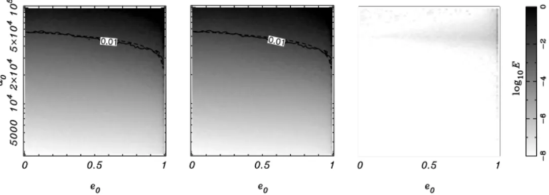
Figure 2. Maximum errorEp(see equation 144) in each cell of thee0–a0plane for the models MAPP (left), LPV2 (middle) and LARKS (right). The solid line curves correspond toEp=0.01 and the dotted curves are the best fits of the level curves.
concerned. Indeed, the best analytical fit of the level curveEp = 0.01 is given by
ac=104.748±0.004(1−e)0.182±0.006, (147)
for the MAPP model and,
ac=104.751±0.003(1−e)0.185±0.005, (148)
for the LPV2 model. These two equations may be considered as identical within the error bounds of the exponents.
For both models the error is essentially due to the averaging of the equations of motion with respect to the mean anomaly. Conversely, the LARKS method is highly reliable in the whole phase-space domain under study, since the error never exceeds 0.01. The effect of the time-step selection rule (146) is clearly visible abovea0 = 50 000 au; the reliability of LARKS is almost conserved whena0 increases.
Speaking about the computation times required to perform all the integrations, the MAPP, LPV2 and LARKS needed 5.5, 1.8 and 75 s, whereas the RA15 integration took 1820 s. Consequently, LPV2 is three times faster than MAPP, and almost 40 times faster than LARKS. All the timing tests were performed without the propaga-tion of the variapropaga-tions vector. Including the tangent maps doubles the computation time for LARKS and MIKLAR with SBABC3 (factors of 2.4 and 2.2, respectively), due to the computation of the tangent Kepler maps (four times per step) and of the tangent perturbation maps (five times per step instead of two usually required for the corrector). The difference in computation time with and without the propagation of variations for LPV2 is smaller (factor of 1.7), thanks to the simplicity of the tangent maps expressions. The difference is even smaller for MAPP (about 1.01) because, based on the Taylor series, it evaluates the Jacobian of the right-hand sides anyway. 5 C O N C L U S I O N S
The two integrators presented in this paper are fast and reliable. Their application range is complementary in two aspects. First, according to the results of Section 4.2.4, we can use LPV2 be-low theEp=0.01 level curve (or its analytical fit given by equa-tion 148), and LARKS above this level curve. This aggregate allows a fast simulation of numerous cometary samples within the assumed 1 per cent accuracy bound. The integrators are also complementary, because if we generate two maps of a chaos indicator values (one with LARKS, and one with LPV), their comparison will immedi-ately show which chaotic zones are due to secular resonances and
which come from the mean motion resonance. The results of such studies will be published in a separate paper. We can already an-nounce that the results of our simulations using the new tools are coherent with that of Brasser (2001).
AC K N OW L E D G M E N T S
The authors appreciate helpful suggestions of Prof. Jacques Laskar concerning the idea and details of using symplectic integrators in the present framework. An anonymous reviewer helped us considerably to improve the paper. MF is grateful to ESA for financial support at INAF–IASF.
R E F E R E N C E S
Barrio R., 2005, Chaos Solitons Fractals, 25, 711 Brasser R., 2001, MNRAS, 324, 1109
Breiter S., 1998, Celest. Mech. Dyn. Astron., 71, 229 Breiter S., Ratajczak R., 2005, MNRAS, 364, 1222 Breiter S., Ratajczak R., 2006, MNRAS, 367, 1808
Deprit A., Elipe A., Ferrer S., 1994, Celest. Mech. Dyn. Astron., 58, 151 Everhart E., 1985, in Carusi A., Valsecchi G. B., eds, ASSL Vol. 115, IAU
Colloq. 83, Dynamics of Comets: Their Origin and Evolution. p. 185 Fouchard M., 2004, MNRAS, 349, 347
Fouchard M., Froeschl´e C., Matese J. J., Valsecchi G., 2005, Celest. Mech. Dyn. Astron., 93, 229
Fouchard M., Froeschl´e C., Valsecchi G., Rickman H. 2006, Celest. Mech. Dyn. Astron., 95, 299
Laskar J., Robutel P., 2001, Celest. Mech. Dyn. Astron., 80, 39 Levison H. F., Dones L., Duncan M. J., 2001, AJ, 121, 2253 McLachlan R. I., Quispel G. R. W., 2002, Acta Numer., 11, 341 Mikkola S., 1997, Celest. Mech. Dyn. Astron., 67, 145
Mikkola S., Innanen K., 1999, Celest. Mech. Dyn. Astron., 74, 59 Mikkola S., Wiegert P., 2002, Celest. Mech. Dyn. Astron., 82, 375 Mikkola S., Palmer P., Hashida Y., 2002, Celest. Mech. Dyn. Astron., 82,
391
Preto M., Tremaine S., 1999, AJ, 118, 2532
Stiefel E. L., Scheifele G., 1971, Linear and Regular Celestial Mechanics. Springer-Verlag, Berlin
Szebehely V., 1967, Theory of Orbits: The Restricted Problem of Three Bodies. Academic Press, New York
Wisdom J., Holman M., 1992, AJ, 104, 2022
Wisdom J., Holman M., Touma J., 1996, Integration Algorithms and Clas-sical Mechanics. AMS, Providence, RI, p. 217
This paper has been typeset from a TEX/LATEX file prepared by the author.