Sequence Learning for Brain Computer Interfaces

(1)

UC San Diego

UC San Diego Electronic Theses and Dissertations

Permalink https://escholarship.org/uc/item/6gn763m3 Author Elango, Venkatesh Publication Date 2017 Peer reviewed|Thesis/dissertation

eScholarship.org Powered by the California Digital Library University of California

(2)

UNIVERSITY OF CALIFORNIA, SAN DIEGO

A Thesis submitted in partial satisfaction of the requirements for the degree

Master of Science in

Electrical Engineering

(Intelligent Systems, Robotics, and Control) by

Venkatesh Elango

Committee in charge:

Professor Vikash Gilja, Chair Professor Bhaskar D. Rao Professor Lawrence K. Saul

(3)

Copyright

(4)

The Thesis of Venkatesh Elango is approved, and it is acceptable in quality and form for publication on microfilm and electronically:

Chair

University of California, San Diego

2017

(5)

TABLE OF CONTENTS

Signature Page . . . iii

Table of Contents . . . iv

List of Figures . . . v

List of Tables . . . vi

Acknowledgements . . . vii

Abstract of the Thesis . . . viii

Chapter 1 Introduction . . . 1

1.1 Background . . . 2

1.2 Related Work and Proposed Solutions . . . 3

1.3 Thesis Structure . . . 4

Chapter 2 Neural Decoding Paradigm . . . 5

2.1 Dataset Description . . . 5

2.2 Decoding Model . . . 6

Chapter 3 Sequence Learning . . . 9

3.1 Hidden Markov Model . . . 9

3.2 Long Short-Term Memory . . . 11

3.2.1 Weight Initialization & Network Architecture . . 12

3.2.2 Curriculum Learning Strategy . . . 13

3.2.3 Hyper-parameter Selection . . . 14

3.3 Results . . . 14

Chapter 4 Sequence Transfer Learning . . . 18

4.1 Transfer Learning Architecture . . . 18

4.2 Results . . . 19

4.3 Visualizing Learned Representation . . . 22

Chapter 5 Conclusions and Future Work . . . 25

Bibliography . . . 29

(6)

LIST OF FIGURES

Figure 3.1: A schematic depicting the Long Short-Term Memory (LSTM) network architecture . . . 11 Figure 3.2: Encoder-decoder architecture for initialization of LSTM

net-work weights. . . 12 Figure 3.3: Unrolled LSTM network with Softmax output at the last time

step for prediction. . . 14 Figure 3.4: Model performance comparison for representative Subject C . . 15 Figure 4.1: A schematic depicting the sequence transfer learning model

ar-chitecture . . . 19 Figure 4.2: Sequence transfer learning model performance comparison for a

representative subject . . . 21 Figure 4.3: Visualizations of learned representation . . . 22

(7)

LIST OF TABLES

Table 3.1: Summary comparing the average accuracy of the LSTM model with existing approaches after 20 random partitions of all the shuffled training data. . . 15 Table 4.1: Summary comparing the average accuracy of transfer learning

with subject specific training, using all training data across 20 random partitions of the shuffled data. . . 21

(8)

ACKNOWLEDGEMENTS

I would like to thank my advisor, Vikash Gilja for welcoming me into the group and giving me the complete flexibility to work on problems that interest me. Your patience, guidance, and sharp insights have helped me a great deal. I am grateful for having the opportunity to work with you.

Aashish Patel, this thesis would not have taken this shape without you. I can not thank you enough for everything that I learned from you. Francis Baek, thanks for your help in getting started with the dataset. Tejaswy Pailla, thank you for all the helpful discussions and feedback over the course of this work. Eugene Arabadzhi and Paolo Gabriel, thank you for your interest in this work and help in presenting it. Janarthanan Rajendran, thank you for listening to my ideas, providing useful suggestions, and reading my thesis and papers at short notices.

I would like to thank all the members of TNEL for creating a wonderful environment and making my stay here fun. I would especially like to thank my parents for their constant support and encouragement.

The chapters in this thesis are adapted from joint work with Aashish Patel, Kai J. Miller, and Vikash Gilja.

(9)

ABSTRACT OF THE THESIS

by

Venkatesh Elango

Master of Science in Electrical Engineering (Intelligent Systems, Robotics, and Control)

University of California, San Diego, 2017

Professor Vikash Gilja, Chair

A fundamental challenge in designing brain-computer interfaces (BCIs) is decoding behavior accurately from time-varying neural oscillations. Studies using BCIs to function as communication prosthesis have demonstrated the plausibility of using these systems for recording neural signals over the long term as well as the ability to decode user intention from these signals. In most scenarios, the decoder used in a BCI is trained specifically for a subject and also has to be trained for every session of use with limited training data. Given these dataset size constraints, the class of decoding algorithms typically explored have restricted

(10)

complexity, often limited to linear models that process neural signals within a fixed duration. However, such constraints can limit the practicality and usability of BCIs.

In this thesis, we investigate the utility of sequential models for decoding behavior from neural signals. To that end, we describe a robust, scalable approach for decoding sequences of neural signals using Long Short-Term Memory (LSTM) networks that work well even when training data is limited. The efficacy of our approach is demonstrated by decoding finger flexion from neural data collected from 4 subjects implanted with electrocorticographic (ECoG) electrode arrays. We also present an architecture for sequence transfer learning, which is able to learn a general representation of the sequential data across subjects, and show that it is able to achieve significant improvements over the state-of-the-models. We believe that these techniques using sequence learning and sequence transfer learning could be applied to the development of many neural systems and may help enable higher performance BCIs.

(11)

Chapter 1 Introduction

A primary goal for brain computer interfaces (BCIs) is to decode intent from neural signals. Neural signals can be collected by placing electrodes on the scalp, the surface of the brain, or intracranially. Neural prosthetic systems can then be designed to predict the intended behavioral actions from these neural signals. Depending on the goal, the decoder in the prosthesis can either have a continuous output (e.g. for use in a motor prosthesis) or a discrete output (e.g for use in a communication prosthesis). Both of these decoders have been implemented for use by people and studies have been performed to test their utility [1, 2]. As quality of life for the patient depends on being able to control the prosthetic naturally and reliably, it is important to be able to decode neural activity accurately. The performance of a decoder is directly related to its ability to overcome noise and account for variability, particularly in situations with constraints on training data availability.

(12)

2

1.1 Background

In the work presented in this thesis, we develop and test decoding algorithms that map Electrocorticography (ECoG) signals to discrete outputs. ECoG signals are measured by implanting ECoG grids subdurally, under the skull and on the surface of the brain. The advantage of ECoG over electroencephalography (EEG), is that it has higher signal-to-noise ratio and has better spatio-temporal resolution. ECoG grids cover different regions of the brain and the placement of the grids differ across subjects. Due to limitations imposed in clinical recording settings, single subject datasets are commonly on the order of minutes to tens of minutes per session and decoders are typically trained for each subject individually, and retrained for each session. Limited by dataset size, existing neural decoders achieve reasonable performance by focusing on constrained decoder designs [2, 3]. As such, the state-of-the art decoders are linear models which only need to learn a small set of parameters [4, 5, 6]. A limitation of these models is that they rely heavily on the quality of the training data, informative features, and often have rigid timing constraints which limit the ability to model neural variability [2]. Furthermore, these specific informative features and timing constraints must be hand-tailored to the associated neural prosthetic task and the corresponding neural activity. On the other hand, deep learning approaches have been applied to similar problems with the goal of learning more robust, distributed representations representations with large amounts of training data [7, 8]. However, only few studies apply these techniques to neural decoding [9, 10].

(13)

3

1.2

1.3 Thesis Structure

This thesis is organized as follows: Chapter 2 describes the existing neu-ral decoding paradigm and the state-of-the-art models. The dataset used in this thesis and the experiment setup are also described in this chapter. Chapter 3 de-scribes the sequence learning problem, existing models, the proposed LSTM based approach. Chapter 4 presents the sequence transfer learning framework and in-vestigates the representations learned by the model. Chapter 5 summarizes the contributions made in the thesis and discusses directions for future work.

(15)

Chapter 2 Neural Decoding Paradigm

Communication prostheses employ discrete decoders to detect the symbol of intent. These decoders typically consider a fixed, finite context [11, 12]. Certain frequency bands, such as 8 - 20 Hz and 70 - 150 Hz, from ECoG signals have been shown to have discriminatory ability from past empirical studies. Signal powers from these bands are extracted and used as features for the discrete decoder. Next, the dataset used for all the analyses done in this thesis is described.

2.1 Dataset Description

Neural signals were recorded from nine patients being treated for medically-refractory epilepsy using standard sub-dural clinical electrocorticography (ECoG) grids. The experiment was a finger flexion task where subjects wearing a data glove were asked to flex a finger for two seconds based on a visual cue [16]. Three subjects were excluded from the analysis due to mismatches in behavioral measurement and cue markers. Rejecting electrodes containing signals that exceed two standard de-viations from the mean signal, two additional subjects are removed from analysis due to insufficient coverage of the sensorimotor region. All subjects participated

(16)

6

in a purely voluntary manner, after providing informed written consent, under ex-perimental protocols approved by the Institutional Review Board of the University of Washington. All patient data was anonymized according to IRB protocol, in accordance with HIPAA mandate. This data has been released publicly [17].

Analyzing the neural data from the four remaining subjects, electrodes are rejected using the same criteria mentioned above. For each subject, 6 - 8 electrodes covering the sensorimotor region are utilized for their importance in motor plan-ning. They are conditioned to eliminate line noise, and then instantaneous spectral power in the high band range (70 - 150 Hz) is extracted for use as the features for the classifier [18]. The data is segmented using only the cue information resulting in 27 - 29 trials per finger (5 classes), with each trial being≈2100ms in length.

2.2 Decoding Model

Since the trials are segmented by cue, a straightforward choice for a finite, fixed context decoder would be one that considers a fixed duration of the neural data after movement onset. The decoder can then be constructed to take in pow-ers, from different frequency bands, over the time period of interest as features. Denoting the feature vector by x and the class label by y, a linear discriminant analysis (LDA) classifier can be used to decode the most likely class label ˆy by

x|y ∼ N(µy,Σy) ˆ

y = arg max

y P(x|y).

The above maximum likelihood formulation can be extended to any generative model by the changing the distribution of P(x|y). While this approach would work well for structured experimental tasks, it cannot be a practical decoder as

(17)

7

the behavior onset is not known in advance. In addition, the rigid timing con-straints imposed by the fixed context decoder limits the usability and flexibility of the prosthesis by the subject. Completely removing these timing constraints would be a free-paced control [19], leading to lower performance and increased decoder complexity. Interaction of the user with decoder can be improved, if these con-straints can be relaxed without degradation of decoder accuracy. For more detailed discussions analysis of this spectrum of user-decoder interaction refer to [20].

Due to the reasons mentioned above, we consider decoders that act on sequential neural data. The signal power for each trial is binned using a non-overlapping window of length 150 ms, yielding an average sequence length of 14 samples. For a typical trial with 2100 ms of data, about 900 ms is prior to the onset of the finger movement and 1200 ms is after the movement onset.

As LDA is commonly used to decode neural signals [6, 12], we use it for making baseline comparisons. For this purpose the signal powers from all the time bins and across the different channels are concatenated into a feature vector. The formulation of LDA using time bins as features has been shown to achieve high accuracies with longer trial lengths [6]. This formulation may be prone to overfit-ting as electrode count and trial duration increase. As such, we emphasize that this formulation results in a strong baseline performance because it can explicitly model the temporal response as a function of neural activity relative to movement onset. This is in contrast to other sequence learning models (HMM and LSTM) for which learned parameters do not change as a function of time relative to move-ment onset and, instead, temporal dynamics are captured by parameters that are constant across time.

(18)

8

Acknowledgement

Chapter 2 is adapted from Venkatesh Elango*, Aashish Patel*, Kai J. Miller, and Vikash Gilja, “Sequence Transfer Learning for Neural Decoding”, Sub-mitted to Neural Information Processing Systems (NIPS), 2017; and Aashish Pa-tel*, Venkatesh Elango*, Kai J. Miller, and Vikash Gilja, “Design considerations for online electrocorticography-based brain-computer interfaces”, in preparation.

(19)

Chapter 3 Sequence Learning

To overcome the limitations in using LDA, we first consider the usage of HMMs for decoding neural signals and then propose an LSTM based decoder. As LDA does not have a representation of time, individual time bins for each electrode were presented as features to the model. Since HMMs and LSTMs do not have that restriction, the sequence data is used as inputs to these models.

3.1 Hidden Markov Model

A hidden Markov model is one of the simplest probabilistic graphical model that can model sequential data. For every time step, in a N-state HMM, the latent state could be one of the N possible states and the observation is obtained from a emission probability distribution conditioned on the latent state. Typically for continuous valued observations, the emission probability is modeled using a Gaussian distribution. The latent state dynamics follow the Markov property where the latent state at the next time step conditioned on the latent state at current time step is independent of the latent state at previous time steps. Thus, the latent state dynamics can be described by a probability transition matrix.

(20)

10

Expectation Maximization (EM) algorithm is used to learn the parameters of the HMM. The EM algorithm is guaranteed to converge, however the non-convexity of the likelihood function implies that there could be multiple possible local optima. To ensure that we converge to a good solution, we initialize the parameters of the emission distributions by learning a Gaussian Mixture Model. As for the transition matrix, we try multiple random initializations and pick the solution that has the maximizes the likelihood of the data.

Since HMMs are generative models to build a decoder, a HMM is learned for each of the classes, and classification decision is done by choosing the class that maximizes the likelihood of the sequence. The HMM baseline decoder is analyzed with 1-state and 2-states using Gaussian emissions to explore if more complex behaviors can be modeled with a more expressive temporal model. While the 2-state HMM is a standard ergodic HMM [21] allowing transitions between both the states, a 1-state HMM is a special case, it does not have any state dynamics and makes an independence assumption for samples across time. Thus, the 1-state HMM is specified by

P({x} |y) = P(x1|y)P(x2|y). . . P(xt|y)

xt|y ∼ N(µy,Σy)

where{x}denotes the sequential data andy denotes the class. We note here that this 1-state HMM is quite similar to the LDA formulation discussed in the previous chapter with notable difference being the assumption of independence across time.

(21)

11

A B

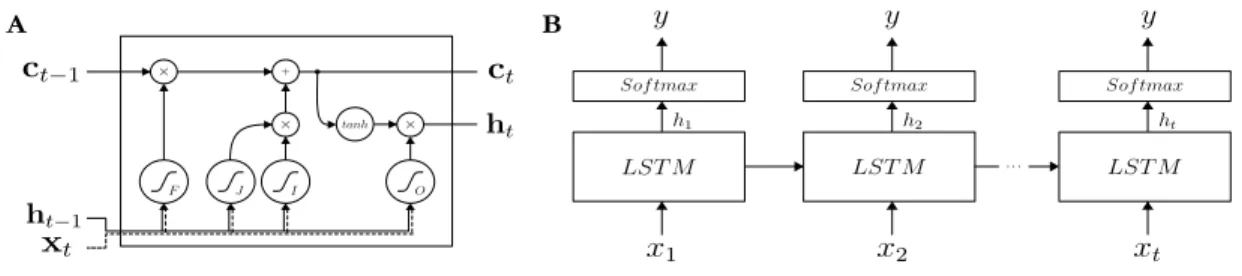
Figure 3.1: A schematic depicting the Long Short-Term Memory (LSTM) network architecture. (A) Gating and activation functions for a single unit. (B) Unrolled LSTM network with Softmax output at every time step during training.

3.2 Long Short-Term Memory

The single recurrent Long Short-Term Memory (LSTM) cell architecture proposed by [22] is utilized and shown in Figure 3.1A. This model is completely specified by ft = σ(Wxfxt+Whfht−1+bf) jt = tanh(Wxjxt+Whjht−1+bj) it = σ(Wxixt+Whiht−1+bi) ot = σ(Wxoxt+Whoht−1+bo) ct = ct−1ft+itjt ht = tanh(ct)ot

whereσ is the sigmoid function, theW terms are weight matrices, thebterms are biases, and represents Hadamard multiplication. To enable gradient flow, the forget gate bias term is initialized to 1 [23, 24]. At every time step during training, the label is provided to allow error propagation during intermediate steps rather than only after the full sequence has been evaluated [25]. This training procedure

(22)

12

x1 x2 xt-1 xt

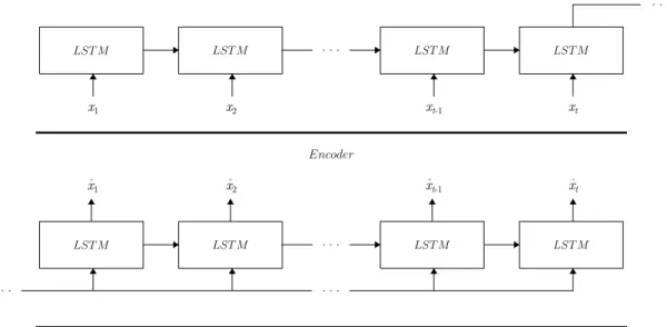
Figure 3.2: Encoder-decoder architecture for initialization of LSTM network weights.

is depicted in Figure 3.1B.

3.2.1 Weight Initialization & Network Architecture

Different weight initialization schemes: random, language model, and se-quence autoencoder [26] were tried. Building on the sese-quence autoencoder, we utilize a modified version where the encoder and decoder weights are not shared, and is similar to the LSTM autoencoder from [27]. This autoencoder architecture is shown in Figure 3.2. Additionally, dropout is utilized in the recurrent states [28] with a probability of 0.3, but is not used on the input layer due to the limited dimensionality of the input. Different model complexities were also explored by varying the number of hidden units as well as by using stacked networks. The model used for all the analyses presented in this thesis was constructed with 100 hidden units, as no performance gain was seen using larger or stacked networks.

(23)

13

While we are able to achieve the same performance using fewer hidden units they take longer to train. Gate recurrent units [15] were also evaluated with no observed improvement in performance.

3.2.2 Curriculum Learning Strategy

Curriculum learning, proposed in [29], shapes the order in which training samples are presented to a neural network in such a way that the difficulty of learning progressively increases. However, it has been shown that in certain task this approach might result in performance that is worse than an approach which does not use curriculum learning [30]. A strategy to overcome this problem is to include training samples of random difficulty with a fixed probability in addition to the samples of increasing difficulty [30]. As this approach presents samples of varying difficult to the network with a certain fixed probability, it is able to generalize better. Defining the difficulty to be directly proportional to the length of the sequence, we use two parameters for shaping the curriculum: r, the rate of increase in difficulty, and p, the probability of selecting a sample of random difficulty. Of the available n training sequences, fraction p of those are selected to be of randoms length drawn from a uniform distribution_U{3, L}, where L is the maximum sequence length. The remaining 1−pfraction of training sequences, are selected to be of a fixed length,l. This length is given by

l = min{r×k+ 3, L}

wherek is the current training epoch, andr, the rate of increase in sequence length per epoch, is between (0,1], ensuring that all training sequences have at least a length of 3. The values for the parameters p and r are chosen to be 1₂ and 1₈

(24)

14

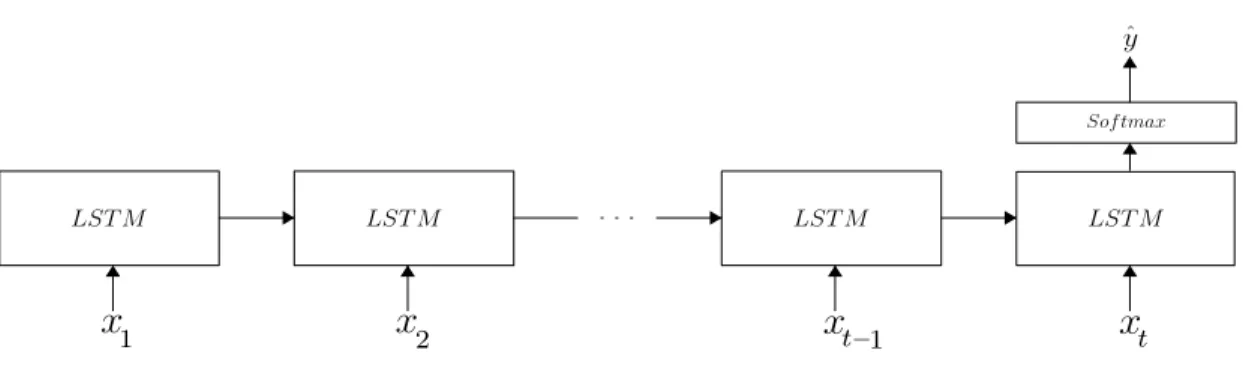
Figure 3.3: Unrolled LSTM network with Softmax output at the last time step for prediction.

respectively. To allow for multiple updates, in every epoch of training the training sequences are split into batches of size 32. If the number of sequences in the entire training set is less than 32, then only one update per epoch is carried out.

3.2.3 Hyper-parameter Selection

The hyper-parameters of the network (number of hidden units, dropout probability) as well as the parameters for curriculum learning (p and r) were selected through optimization on a single patient, Subject B, and used for all sub-jects. To prevent overfitting to the training set, training was stopped at 75 epochs for all evaluations and all subjects. Models were trained through backpropagation using Adam [31] and prediction is performed on the test data with accuracies re-ported using classification at the last time step, except when specified otherwise. This prediction setup is shown in Figure 3.3.

3.3 Results

We found that LSTMs trained on an individual subject perform compara-ble to state-of-the-art models with sufficient training samples. Additionally, using

(25)

15

A B

0 5 10 15 20 25

Training Samples per Class

0 0.1 0.2 0.3 0.4 0.5 0.6 0.7 0.8 0.9 1 Classi fi cation Accura cy LSTM LDA HMM - 1s HMM - 2s -800 -600 -400 -200 0 200 400 600 800 1000 1200

Time Relative to Movement Onset (ms)

0 0.1 0.2 0.3 0.4 0.5 0.6 0.7 0.8 0.9 1 Classi fi cation Accura cy LSTM LDA HMM - 1s HMM - 2s

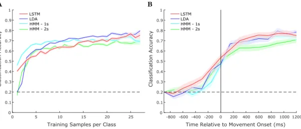
Figure 3.4: Model performance comparison for representative Subject C. (A) Accuracy as a function of the amount of training samples and (B) Accuracy as a function of time with respect to movement onset evaluated for different models and using all available training data. Error bars show standard error of mean using 20 random partitions of the shuffled data.

Table 3.1: Summary comparing the average accuracy of the LSTM model with existing approaches after 20 random partitions of all the shuffled training data.

Model Subject A Subject B Subject C Subject D

LDA 0.50 0.53 0.79 0.64

HMM - 1s 0.51 0.61 0.69 0.65

HMM - 2s 0.53 0.59 0.68 0.60

LSTM 0.51 0.62 0.75 0.69

the proposed transfer learning framework, we note that LSTMs provide a princi-pled, robust, and scalable approach for decoding neural signals that can exceed performance of state-of-the-art models.

When model accuracy is evaluated as a function of the number of training samples, shuffled data is randomly partitioned into train and test sets according to the evaluated training sample count. A validation set is not used due to the limited data size. For all subjects and experiments, the test set comprising of at least 2 samples per class. All experiments report the average of 20 random partitions of the shuffled data.

(26)

16

First we establish the performance of the baseline models (Table 3.1). In-terestingly, we observe that increasing the complexity of the HMM marks little improvement in the classification accuracy and typically results in decreased ac-curacy at low sample counts due to the increased complexity. Additionally, while LDA performs comparably for three subjects, it performs much better than the other models for Subject C due to the increased alignment between cue and ob-served behavior. This is expected because, as noted, the LDA formulation is better suited to take advantage of the time alignment in the experiment.

Examining the performance of the LSTMs (Table 3.1), we demonstrate that the proposed model is better able to extract information from the temporal variability in the signals than HMMs and is able to achieve performance comparable to the best baseline for each of the subjects. Consequently, we observe across most subjects LSTMs are able to exceed performance of both HMM models and LDA. Even for Subject C, the LSTM model is comparable to LDA without making the temporal alignment assumption.

Further investigating model time dependence, accuracy is evaluated using neural activity preceding and following behavioral onset. As LDA explicitly models time, a series of models for each possible sequence length are constructed. Depicted in Figure 3.4B, we observe that the LSTM is slightly better able to predict the behavioral class at earlier times compared to HMMs and is comparable to LDA across all times.

Acknowledgement

Chapter 3 is adapted from Venkatesh Elango*, Aashish Patel*, Kai J. Miller, and Vikash Gilja, “Sequence Transfer Learning for Neural Decoding”, Sub-mitted to Neural Information Processing Systems (NIPS), 2017; and Aashish

(27)

Pa-17

tel*, Venkatesh Elango*, Kai J. Miller, and Vikash Gilja, “Design considerations for online electrocorticography-based brain-computer interfaces”, in preparation.

(28)

Chapter 4 Sequence Transfer Learning

4.1 Transfer Learning Architecture

We next explored the possibility of transferring the representation learned by the LSTM from a subject, S1, onto a new subject, S2. Typical transfer learn-ing approaches keep the lower-level layers fixed, but re-train the higher-level lay-ers [27, 32]. Due to the unique electrode coverage and count as well as physiological variability across subjects, this approach would not work in this problem. Account-ing for these factors, we propose usAccount-ing an affine transformation to project the data from S2 onto the input of an LSTM trained on S1 as we might expect a similar mixture of underlying neural dynamics across subjects. The fully connected affine transformation is specified by

xS 0 2

t = WxxxSt2 +bx

whereWx andbx are the weights and biases of the affine mapping,xSt2 and x S02

t are the original and the transformed sequential data fromS2 respectively.

Using hyper-parameters outlined in the single subject LSTM model, a

(29)

19

A B

Step 1 Step 2 Step 1 Step 2

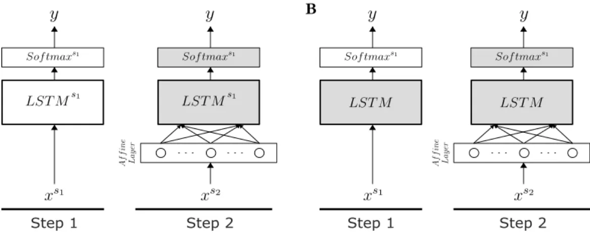
Figure 4.1: A schematic depicting the LSTM transfer learning model archi-tecture. Gray indicates fixed and white indicates learned weights, both (A) and (B) depict a 2-step training process with Subject 1 (S1) training in step 1 and

Subject 2 (S2) training of only the affine layer in step 2. (A) Transfer learning

model (TL) training the LSTM and Softmax layers for S1 in step 1. (B)

Ran-domly initialized LSTM layer and training only the Softmax layer forS1in step

1.

step training process, shown in Figure 4.1A, is utilized. The first step trains the LSTM using all of the data from S1. Upon fixing the learned weights, the fully connected affine layer is attached to the inputs of the LSTM and trained on S2 data. To establish that the affine transformation is only learning an input mapping and not representing the neural dynamics, a baseline comparison is utilized where the Step 1 LSTM is fixed to a random initialization and only the Sof tmaxS1 _is

trained, this is shown in Figure 4.1B.

4.2 Results

Historically, neural prostheses must be tuned frequently for individual sub-jects to account for neural variability [1, 33]. Establishing LSTMs as a suitable model for decoding neural signals, we explored their ability to learn more robust, generalized representations that can be utilized across subjects.

(30)

20

We demonstrate that learning the affine transformation for the input, it is possible to relax the constraint of knowing exactly where the electrodes are located without having to retrain the entire network. First examining the baseline condition in order to assess the ability for the affine layer to learn the underlying neural dynamics, the S1 LSTM weights were randomly initialized and fixed as outlined in Figure 4.1B. Looking at Figure 4.1A, the model performs slightly above chance, but clearly is unable to predict behavior from the data. The TL model where only the affine layer is trained in Step 2 forS2 (Figure 4.1A) performs comparably to the subject specific model for S2. The notable advantage provided by TL is that there is an increase in loss stability over epochs, which indicates a robustness to overfitting. Finally, relaxing the fixed LST MS1 _and _{Sof tmax}S1

constraints, we demonstrate that the TL-Finetuned model achieves significantly better accuracy than both the best linear model and subject specific LSTM.

Detailing the performance for each TL and TL-Finetuned, we evaluate all 3 remaining subjects for each S2. For the TL model, we found that the transfer between subjects is agnostic of S1 specific training and performs similarly across all 3 subjects. The performance of TL-Finetuned is similarly evaluated, but has trends unique to TL. In particular, we observe that transferring from Subject A always provides the best results followed by transferring from Subject B. Accuracies using the maximum permissible training data for all four subjects comparing the two transfer learning approaches and the best linear model as well as the subject specific LSTM are reported in Table 4.1.

(31)

21

0 5 10 15 20 25

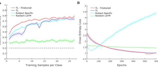
Training Samples per Class 0 0.1 0.2 0.3 0.4 0.5 0.6 0.7 0.8 0.9 1 Classi fi cation Accura cy TL - Finetuned TL Subject Specific Random LSTM 0 100 200 300 400 500 600 Epochs 0.5 1 1.5 2 2.5 3 3.5 4 4.5 5 Cros s-Entr opy Loss TL - Finetuned TL Subject Specific Random LSTM A B

Figure 4.2: Transfer learning LSTM performance comparison for a represen-tative subject. The TL-Finetuned, TL, and random LSTM all utilize Subject B as S1 and Subject C as S2. The subject specific model uses Subject C. (A)

Accuracy as a function of the amount of training samples. (B) Cross-entropy loss across epochs, using 10 training samples per class. Error bars show stan-dard error of mean averaging results from 20 random partitions of the shuffled data.

Table 4.1: Summary comparing the average accuracy of transfer learning with subject specific training, using all training data across 20 random partitions of the shuffled data.

Model Subject A Subject B Subject C Subject D Best Linear Classifier 0.53 0.61 0.79 0.65

Subject Specific 0.51 0.62 0.75 0.69 TL (S1 = Subject A) - 0.66 0.72 0.60 TL (S1 = Subject B) 0.40 - 0.70 0.46 TL (S1 = Subject C) 0.44 0.63 - 0.59 TL (S1 = Subject D) 0.44 0.67 0.73 -TL-Finetuned (S1 = Subject A) - 0.71 0.82 0.70 TL-Finetuned (S1 = Subject B) 0.46 - 0.75 0.62 TL-Finetuned (S1 = Subject C) 0.44 0.63 - 0.66 TL-Finetuned (S1 = Subject D) 0.53 0.71 0.79

(32)

-22 A B Subject 1 Subject 2 RMotor RMotor RSensory ROccipi tal

RMotor RSensory RMotor RSensory

TL TL - Finetuned Subject 1 Subject 2 0 ms 450 ms 900 ms

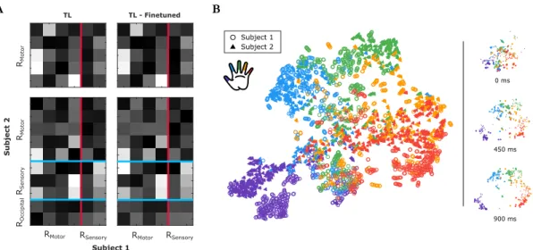
Figure 4.3: Visualizations of learned representation. (A) Weights of the learned affine mapping from Subject 2 (Subject C) to Subject 1 (Subject B). Electrodes mapped from motor to sensorimotor and sensorimotor + occipital to sensorimotor regions of S2 to S1, respectively. Both TL and TL-Finetuned

weights are depicted. (B) Two-dimensional t-SNE embedding of the learned signal representation corresponding to different fingers for both subjects.

4.3 Visualizing Learned Representation

For the transfer learning models, we explored the stability of the affine layer and analyzed the learned LSTM weights between subjects. Examining the learned weights of the affine mapping layer, we can see that the mapping resembles a pro-jection of electrodes to the appropriate brain regions. In Figure 4.3A, we show the learned affine transformations for two cases: a projection from sensorimotor (RM otor, RSensory) between the two subjects, and a projection also adding the oc-cipital lobe electrodes (ROccipital) for S2. As the occipital lobe is involved with integrating visual information, it is not as informative for motor movement tasks. Therefore, we would expect, and in fact observe, there to be an affine transforma-tion with weights for ROccipital closer to zero indicating an absence of electrodes inS1 that contain similar information. Additionally, we can qualitatively observe

(33)

23

the stability of the affine transform after the fixed LST MS1 _and _{Sof tmax}S1 _are

relaxed. It is clear by looking between the left and right columns of Figure 4.3A that the learned weights from TL are a good representation and only require minor modification in TL-Finetuned.

Furthermore, exploring the use of LSTMs for transfer learning, a two-dimensional embedding of the LSTM output using t-SNE [34] on the training data was created. The t-SNE embedding is produced by first converting the pair-wise Euclidean distances, dij, in the high-dimensional space to joint probabilities

pij ∝ exp(−d2ij). In the two-dimensional space, the joint probabilities, qij, is modelled by a heavy tailed distribution qij ∝ (1 +d2ij)

−1_{. The mapping from the} high-dimensional space to the two-dimensional space is obtained by minimizing the Kullback-Leibler divergence between the joint probability distribution in the high-dimensional space and the joint probability distribution in the two-high-dimensional space. This minimization of the Kullback-Leibler divergence is performed by gra-dient descent on the cost function [34].

We use theLST MS1 _{outputs for}_S

1 data andLST MS1 outputs forS2 data after passing it through the learned affine layer onS2. All the data between -300 ms to 900 ms, relative to behavioral onset, is embedded in the two-dimensional space. From the summary image, Figure 4.3B, it is clear that the model is able to separate classes for both subjects well and that the projections for both the subjects are clustered together. To identify the source of the confusion between labels in the two-dimensional embedding, we project the output at different time steps and see that the majority of the confusion occurs at the start of the sequences.

(34)

24

Acknowledgement

Chapter 4 is adapted from Venkatesh Elango*, Aashish Patel*, Kai J. Miller, and Vikash Gilja, “Sequence Transfer Learning for Neural Decoding”, Sub-mitted to Neural Information Processing Systems (NIPS), 2017.

(35)

Chapter 5 Conclusions and Future Work

In this work, we have shown that LSTMs can efficiently model the time-varying dynamics within a neural sequence and are a good alternative to state-of-the-art linear decoders. Even with a low sample count and comparably greater number of parameters, the model is able to extract useful information without overfitting. Moreover, LSTMs provide a robust framework that is capable of scaling with large sample counts as opposed to the the limited scalability provided by linear classifiers.

Establishing the LSTM as a good approach for neural decoding, we pro-posed a sequence transfer learning framework for utilizing the model in transfer learning scenarios. We started by using a constrained model where the weights of LSTM and Softmax are learned on one subject and transferred onto another subject. For the new subject, an affine layer feeding into the input of the LSTM is learned and the rest of the weights are kept fixed. We next considered a less constrained model where the LSTM weights are also allowed to be trained. The performance of this model is shown to exceed that of both the subject specific training and the best linear decoder models across all subjects. This robustness

(36)

26

against subject specific neural dynamics even when only the affine transform is learned indicates that the LSTM is capable of extracting useful information that generalizes to the new patient with limited impact due to the original subject’s relative performance. Looking at the tradeoffs between TL and TL-Finetuned, the latter is able to achieve performance that exceeds the current state-of-the-art models with fewer subject-specific training samples while the former does not nec-essarily provide an accuracy that exceeds the subject specific model. However, because TL only requires training of the affine layer, the training is less compu-tationally expensive than training TL-Finetuned. From Figure 4.2B, it could be seen when learning only the affine transformation the cross-entropy loss is still decreasing after 500 epochs. This suggests that with better optimization methods, the TL model by itself may outperform the subject-specific model. This indicates that the LSTM is capable of extracting a representation of the neural variability between behaviors that generalizes across patients. While this may be specific to the behavior being measured, it posits potential scenarios for using sequence transfer learning.

Exploring the versatility of the affine layer, we consider relaxing the struc-tured mapping of electrodes between the patients and instead, for the transferred subject, allow feeding in electrodes from non-informative region or removal of a subset of electrodes from the informative region. While the structured mapping would intuitively yield good results if electrode placement is the sole factor influ-encing neural variability, we see that it leads to suboptimal performance due to limited alignment capabilities as well as the underlying neural representation be-ing unique. The addition of an affine layer, however, provides sufficient flexibility for the input remapping to account for this variability and matches the new sub-jects input electrodes based on error minimization. Moreover, backpropagation is

(37)

27

able to optimize the weights regardless ofS2 input dimensionality and thus allows for eliminating use of non-informative electrodes. This input transformation layer leads to model training stability and is shown to be a valid mapping due to the min-imal weight update when transitioning from TL to TL-Finetuned. Furthermore, exploring the relationship between subjects 1 and 2, the t-SNE analysis shows that the learned parameters for the affine layer provide a meaningful mapping between the two patients.

Considering the limitations imposed on our model by stopping at a fixed evaluation epoch, it would be possible to further boost performance by utilizing early stopping with a validation set. As a future work, we would like to extend the sequence transfer learning model to learn the representation in the network across multiple subjects by casting this as a multi-task learning problem. While the input features were selected from empirical observations made in previous studies, the results could be improved by extracting the features in an unsupervised manner using autoencoders [35] or by training the decoder end-to-end using convolutional LSTMs [36, 37]. Another possible future direction is to use this framework for decoding a continuous variable such as cursor position or finger flexion trace, as they could be of use in a motor BCI.

We believe that the approaches established in this thesis provide techniques for decoding neural signals that had not yet been explored in detail. Particularly, the insights gained from exploring neural decoding leveraging the expressibility and generalizability of LSTMs yielded techniques that provide more accurate and robust models compared to current state-of-the-art decoders. Consequently, the strategies of applying LSTMs to sequence learning and sequence transfer learning problems will be useful in a variety of neural systems.

(38)

28

Acknowledgement

Chapter 5 is adapted from Venkatesh Elango*, Aashish Patel*, Kai J. Miller, and Vikash Gilja, “Sequence Transfer Learning for Neural Decoding”, Sub-mitted to Neural Information Processing Systems (NIPS), 2017.

(39)

Bibliography

[1] Chethan Pandarinath, Paul Nuyujukian, Christine H Blabe, Brittany L Sorice, Jad Saab, Francis R Willett, Leigh R Hochberg, Krishna V Shenoy, and Jaimie M Henderson. High performance communication by people with paral-ysis using an intracortical brain-computer interface. eLife, 6:e18554, 2017. [2] Mariska J Vansteensel, Elmar GM Pels, Martin G Bleichner, Mariana P

Branco, Timothy Denison, Zachary V Freudenburg, Peter Gosselaar, Sacha Leinders, Thomas H Ottens, Max A Van Den Boom, et al. Fully implanted brain–computer interface in a locked-in patient with als.New England Journal

of Medicine, 375(21):2060–2066, 2016.

[3] Takufumi Yanagisawa, Masayuki Hirata, Youichi Saitoh, Haruhiko Kishima, Kojiro Matsushita, Tetsu Goto, Ryohei Fukuma, Hiroshi Yokoi, Yukiyasu Kamitani, and Toshiki Yoshimine. Electrocorticographic control of a pros-thetic arm in paralyzed patients. Annals of neurology, 71(3):353–361, 2012. [4] Vikash Gilja, Paul Nuyujukian, Cindy A Chestek, John P Cunningham, M Yu

Byron, Joline M Fan, Mark M Churchland, Matthew T Kaufman, Jonathan C Kao, Stephen I Ryu, et al. A high-performance neural prosthesis enabled by control algorithm design. Nature neuroscience, 15(12):1752–1757, 2012. [5] Jennifer L Collinger, Brian Wodlinger, John E Downey, Wei Wang,

Eliza-beth C Tyler-Kabara, Douglas J Weber, Angus JC McMorland, Meel Velliste, Michael L Boninger, and Andrew B Schwartz. High-performance neuropros-thetic control by an individual with tetraplegia. The Lancet, 381(9866):557– 564, 2013.

[6] Guy Hotson, David P McMullen, Matthew S Fifer, Matthew S Johannes, Kapil D Katyal, Matthew P Para, Robert Armiger, William S Anderson, Nitish V Thakor, Brock A Wester, et al. Individual finger control of a modular prosthetic limb using high-density electrocorticography in a human subject.

Journal of neural engineering, 13(2):026017, 2016.

[7] Alex Graves, Abdel-rahman Mohamed, and Geoffrey Hinton. Speech recog-nition with deep recurrent neural networks. In Acoustics, speech and signal

(40)

30

processing (icassp), 2013 ieee international conference on, pages 6645–6649.

IEEE, 2013.

[8] Ilya Sutskever, Oriol Vinyals, and Quoc V Le. Sequence to sequence learning with neural networks. In Advances in neural information processing systems, pages 3104–3112, 2014.

[9] Pouya Bashivan, Irina Rish, Mohammed Yeasin, and Noel Codella. Learning representations from eeg with deep recurrent-convolutional neural networks.

arXiv preprint arXiv:1511.06448, 2015.

[10] David Sussillo, Sergey D Stavisky, Jonathan C Kao, Stephen I Ryu, and Krishna V Shenoy. Making brain–machine interfaces robust to future neural variability. Nature Communications, 7, 2016.

[11] Cynthia A Chestek, Vikash Gilja, Christine H Blabe, Brett L Foster, Kr-ishna V Shenoy, Josef Parvizi, and Jaimie M Henderson. Hand posture clas-sification using electrocorticography signals in the gamma band over human sensorimotor brain areas. Journal of neural engineering, 10(2):026002, 2013. [12] Tejaswy Pailla, Werner Jiang, Benjamin Dichter, Edward F Chang, and

Vikash Gilja. Ecog data analyses to inform closed-loop bci experiments for speech-based prosthetic applications. InEngineering in Medicine and Biology

Society (EMBC), 2016 IEEE 38th Annual International Conference of the,

pages 5713–5716. IEEE, 2016.

[13] Zuoguan Wang, Gerwin Schalk, and Qiang Ji. Anatomically constrained de-coding of finger flexion from electrocorticographic signals. In Advances in

neural information processing systems, pages 2070–2078, 2011.

[14] Tobias Wissel, Tim Pfeiffer, Robert Frysch, Robert T Knight, Edward F Chang, Hermann Hinrichs, Jochem W Rieger, and Georg Rose. Hidden markov model and support vector machine based decoding of finger move-ments using electrocorticography.Journal of neural engineering, 10(5):056020, 2013.

[15] Kyunghyun Cho, Bart Van Merri¨enboer, Dzmitry Bahdanau, and Yoshua Bengio. On the properties of neural machine translation: Encoder-decoder approaches. arXiv preprint arXiv:1409.1259, 2014.

[16] Kai J Miller, Dora Hermes, Christopher J Honey, Adam O Hebb, Nick F Ramsey, Robert T Knight, Jeffrey G Ojemann, and Eberhard E Fetz. Human motor cortical activity is selectively phase-entrained on underlying rhythms.

(41)

31

[17] Kai J Miller and Jeffrey G Ojemann. A library of human electrocorticographic data and analyses. In 2016 Neuroscience Meeting Planner. Society for Neu-roscience, 2016.

[18] Kai J Miller, Eric C Leuthardt, Gerwin Schalk, Rajesh PN Rao, Nicholas R Anderson, Daniel W Moran, John W Miller, and Jeffrey G Ojemann. Spectral changes in cortical surface potentials during motor movement. Journal of

Neuroscience, 27(9):2424–2432, 2007.

[19] Neil Achtman, Afsheen Afshar, Gopal Santhanam, M Yu Byron, Stephen I Ryu, and Krishna V Shenoy. Free-paced high-performance brain–computer interfaces. Journal of neural engineering, 4(3):336, 2007.

[20] Aashish N Patel. Towards Practical Neural Prosthetic Interfaces. M.S. Thesis, University of California, San Diego, 2017.

[21] Lawrence R Rabiner. A tutorial on hidden markov models and selected appli-cations in speech recognition. Proceedings of the IEEE, 77(2):257–286, 1989. [22] Sepp Hochreiter and J¨urgen Schmidhuber. Long short-term memory. Neural

computation, 9(8):1735–1780, 1997.

[23] Felix A Gers, J¨urgen Schmidhuber, and Fred Cummins. Learning to forget: Continual prediction with lstm. Neural computation, 12(10):2451–2471, 2000. [24] Rafal Jozefowicz, Wojciech Zaremba, and Ilya Sutskever. An empirical ex-ploration of recurrent network architectures. In Proceedings of the 32nd

In-ternational Conference on Machine Learning (ICML-15), pages 2342–2350,

2015.

[25] Joe Yue-Hei Ng, Matthew Hausknecht, Sudheendra Vijayanarasimhan, Oriol Vinyals, Rajat Monga, and George Toderici. Beyond short snippets: Deep networks for video classification. In Proceedings of the IEEE conference on

computer vision and pattern recognition, pages 4694–4702, 2015.

[26] Andrew M Dai and Quoc V Le. Semi-supervised sequence learning. In

Ad-vances in Neural Information Processing Systems, pages 3079–3087, 2015.

[27] Nitish Srivastava, Elman Mansimov, and Ruslan Salakhudinov. Unsupervised learning of video representations using lstms. InInternational Conference on

Machine Learning, pages 843–852, 2015.

[28] Yarin Gal and Zoubin Ghahramani. A theoretically grounded application of dropout in recurrent neural networks. In Advances in Neural Information

(42)

32

[29] Yoshua Bengio, J´erˆome Louradour, Ronan Collobert, and Jason Weston. Cur-riculum learning. In Proceedings of the 26th annual international conference

on machine learning, pages 41–48. ACM, 2009.

[30] Wojciech Zaremba and Ilya Sutskever. Learning to execute. arXiv preprint

arXiv:1410.4615, 2014.

[31] Diederik Kingma and Jimmy Ba. Adam: A method for stochastic optimiza-tion. arXiv preprint arXiv:1412.6980, 2014.

[32] Jason Yosinski, Jeff Clune, Yoshua Bengio, and Hod Lipson. How transferable are features in deep neural networks? In Advances in neural information

processing systems, pages 3320–3328, 2014.

[33] JD Simeral, Sung-Phil Kim, MJ Black, JP Donoghue, and LR Hochberg. Neural control of cursor trajectory and click by a human with tetraplegia 1000 days after implant of an intracortical microelectrode array. Journal of

neural engineering, 8(2):025027, 2011.

[34] Laurens van der Maaten and Geoffrey Hinton. Visualizing data using t-sne.

Journal of Machine Learning Research, 9(Nov):2579–2605, 2008.

[35] Quoc V Le, Marc’Aurelio Ranzato, Rajat Monga, Matthieu Devin, Kai Chen, Greg S Corrado, Jeff Dean, and Andrew Y Ng. Building high-level features using large scale unsupervised learning.arXiv preprint arXiv:1112.6209, 2011. [36] Xingjian Shi, Zhourong Chen, Hao Wang, Dit-Yan Yeung, Wai-kin Wong, and Wang-chun Woo. Convolutional lstm network: A machine learning approach for precipitation nowcasting. In Advances in Neural Information Processing

Systems, pages 802–810, 2015.

[37] Yu Zhang, William Chan, and Navdeep Jaitly. Very deep convolutional net-works for end-to-end speech recognition. arXiv preprint arXiv:1610.03022, 2016.