Maximum similarity based feature matching and adaptive multiple kernel learning for object recognition

(1)

MAXIMUM SIMILARITY BASED FEATURE

MATCHING AND ADAPTIVE MULTIPLE KERNEL

LEARNING FOR OBJECT RECOGNITION

by

Ziming Zhang

B.Eng., Northeastern University, 2005

A THESIS SUBMITTED IN PARTIAL FULFILLMENT OF THE REQUIREMENTS FOR THE DEGREE OF

MASTER OFSCIENCE in the School of Computing Science c Ziming Zhang 2010 SIMON FRASER UNIVERSITY

Spring 2010

(2)

Name: Degree: Title of thesis: Examining Committee: Date Approved: Ziming Zhang Master of Science

Maximum Similarity Based Feature Matching and Adap-tive Multiple Kernel Learning for Object Recognition

Dr. Stella Atkins Chair

Dr. Ze-NianLi,Co-Senior Supervisor

Dr. Mark S. Drew, Co-Senior Supervisor

Dr. Greg Mori, SFU Examiner

1../0

---,--b

_r

d

~

I

2-01'0

(3)

Last revision: Spring 09

Declaration of

Partial Copyright Licence

The author, whose copyright is declared on the title page of this work, has granted to Simon Fraser University the right to lend this thesis, project or extended essay to users of the Simon Fraser University Library, and to make partial or single copies only for such users or in response to a request from the library of any other university, or other educational institution, on its own behalf or for one of its users. The author has further granted permission to Simon Fraser University to keep or make a digital copy for use in its circulating collection (currently available to the public at the “Institutional Repository” link of the SFU Library website <www.lib.sfu.ca> at: <http://ir.lib.sfu.ca/handle/1892/112>) and, without changing the content, to translate the thesis/project or extended essays, if technically possible, to any medium or format for the purpose of preservation of the digital work.

The author has further agreed that permission for multiple copying of this work for scholarly purposes may be granted by either the author or the Dean of Graduate Studies.

It is understood that copying or publication of this work for financial gain shall not be allowed without the author’s written permission.

Permission for public performance, or limited permission for private scholarly use, of any multimedia materials forming part of this work, may have been granted by the author. This information may be found on the separately catalogued multimedia material and in the signed Partial Copyright Licence.

While licensing SFU to permit the above uses, the author retains copyright in the thesis, project or extended essays, including the right to change the work for subsequent purposes, including editing and publishing the work in whole or in part, and licensing other parties, as the author may desire.

The original Partial Copyright Licence attesting to these terms, and signed by this author, may be found in the original bound copy of this work, retained in the Simon Fraser University Archive.

Simon Fraser University Library Burnaby, BC, Canada

(4)

In this thesis, we perform object recognition using (i) maximum similarity based feature matching, and (ii) adaptive multiple kernel learning. Images are likely more similar if they contain objects within the same categories, so how to measure image similarities correctly and efficiently is one of the critical issues for object recognition. We first propose to match features between two images so that their similarity is maximized, and employ support vector machines (SVMs) for recognition based on the maximum similarity matrix. Sec-ondly, given several similarity matrices (kernels) created by different visual information in images, we propose a novel adaptive multiple kernel learning technique to generate an opti-mal kernel from all the kernels based on biconvex optimization. These two new approaches are tested on the most recent image benchmark datasets and their results are impressive, equalling or bettering the state-of-the-art results.

Key words:Object recognition; Maximum similarity; Feature matching; Adaptive mul-tiple kernel learning

(5)

for my parents

(6)

I would like to take this opportunity to thank my two supervisors, Professor Ze-Nian Li and Professor Mark Drew, for all their great help and advices during my studies in Simon Fraser University. Meanwhile, I would like to thank Professor Greg Mori to be my Examiner, my colleagues Dr. Yang Wang, Jiawei Huang, Weilong Yang, and many others at Vision and Media Lab, and all my friends for their suggestions and care.

Finally, I would like to thank my family for their understanding and support.

(7)

List of Tables

3.1 Performance comparison betweenw= 0.5and the bestwfor differentkintervals (%). . . 20 3.2 Comparison results between different approaches on Graz-01 (%) . . . 29 3.3 Comparison results between different approaches on Graz-02 (%) . . . 30

4.1 Comparison between the computational time (/s) on training different MKL approaches using Caltech-101 in the form of (mean±standard deviation). . . 45

(10)

1.1 40 samples from the first 40 categories in the Caltech-256, one sample per category. . . . 2

3.1 Illustration of the intuition of the maximum similarity measure. . . 12 3.2 Intuition of multiplication of the feature similarity, the global feature structure similarity,

and the feature correspondence occurrence prior. . . 15 3.3 An example of feature correspondence between setA with 4 points and set B with 6

points. Here, green dots represent the unmatched points in each set, red dots represent the matched point pairs connected by blue dotted lines, and the yellow dotb0is for no match cases which does not belong toB. The constrained global spatial structure for point a1(reps. b2) consists of the normalized distances and the normalized angles betweena1 (reps.b2) and each matched point in the set. . . 16 3.4 Mismatching percentages (%) vs. parameterwusing differentkintervals for (a) “Hotel”

and (b) “House” sequences. . . 20 3.5 Our result for matching the first and last frames (k= 100) of the “hotel” sequence, where

green lines indicate the correct feature correspondences, and the red lines indicate the wrong ones. Left: Ground truth of the feature correspondences predefined in the two images.Right: Our result (accuracy:14/30 = 46.7%) withw= 0.5. . . 21 3.6 Our result for matching the first and last frames (k = 110) of the “house” sequence,

where green and red lines have the same meanings as Fig. 3.5. Left: Ground truth of the feature correspondences predefined in the two images. Right: Our result (accuracy: 12/30 = 40.0%) withw= 0.5. . . 21

(11)

3.7 Illustration of matching two images. Each image is represented as a collection of fea-tures of the patches. Weights (red) on the edges (green) denote the matching probabilities between the feature pairs so that the similarity between the two images is obtained.. . . . 23 3.8 Performance comparison on Graz-01 between different PFM with differentC. . . 29 3.9 Performance comparison on Graz-02 between different PFM with differentC. . . 30

4.1 Comparison between a typical general MKL approach proposed in [37] and B-AdaMKL. . 38 4.2 MKL comparison on Caltech-101 using descriptors of (a) GB, (b) SIFT, and (c) GB+SIFT.

`1and`2in the figures denote`1-norm and`2-norm of kernel coefficients. Clearly, our biconvex optimization based AdaMKL approaches are consistently comparable to SMKL and GMKL, which are both convex optimization based MKL approaches. . . 43 4.3 An example of comparison of the learned kernel coefficients between (a) SMKL, (b)

GMKL, (c)`1-norm B-AdaMKL, (d)`2-norm B-AdaMKL, (e)`1-norm M-AdaMKL, and (f)`2-norm M-AdaMKL after`1 normalization using GB+SIFT and 15 training images per category. In (a), (b), (c), and (d), thex-axis denotes the index of each object category in Caltech-101, and they-axis denotes 10-scale, 20-scale, and 30-scale GB descriptors plus 10-scale, 20-scale, and 30-scale SIFT descriptors in order from top to bottom. In (e) and (f), the figures show the shared kernel coefficients for all the categories. . . 43 4.4 MKL comparison on Average Learning Time (ALT) in seconds on kernel coefficients on

Caltech-101 using descriptors of (a) GB, (b) SIFT, and (c) GB+SIFT. On the curves, the lower parts of standard deviation of GMKL using 15 training images per category in (b) and using 10 training images in (c) are missing, because the values are negative. . . 44 4.5 Our results on Caltech-101 using`1-norm M-AdaMKL. (a) Result comparison based on

different descriptors. (b) Result comparison between ours and some other published ap-proaches. From top to bottom, the corresponding references are [11, 69, 41, 53, 28, 30, 24, 25, 68, 31, 23]. Notice that the approaches with the mark “*” used different training and test methods from ours. Precisely, using all the descriptors,`1-norm M-AdaMKL achieves the mean accuracies of(27.3±4.1)%,(53.6±0.4)%,(63.4±0.2)%,(67.2±1.4)%, (70.1±1.3)%,(72.1±1.7)%, and(74.4±0.5)%, respectively in order. . . 46

(12)

proaches. From top to bottom, the corresponding references are [30, 11, 68, 24, 10, 61, 53]. Precisely, using all the descriptors,`1-norm M-AdaMKL achieves the mean accuracies of (8.8±0.8)%,(21.2±0.3)%,(27.9±0.6)%,(31.4±1.0)%,(33.2±0.8)%,(34.7±1.2)%, (36.4±1.7)%, and(41.5±1.2)%respectively in order. . . 47

(13)

List of Algorithms

3.1 Polynomial-time Approximate Algorithm for Maximization . . . 19 4.1 Alternative Parameter Updating Algorithm for B-AdaMKL . . . 39

(14)

Introduction

Object recognition in computer vision aims to emulate one of the most essential functional-ities of human vision to help machines recognize objects in the environments automatically. According to the data which contain objects, object recognition can be performed in 2D im-ages, 3D videos, 4D medical data, etc. This thesis focuses on recognizing objects in imim-ages, specifically, recognizing the categories of objects rather than recognizing (or detecting) spe-cific objects or identifying objects. For example, as long as there exists an instance of bike with a reasonable scale in an image, no matter where or at what scale the bike instance is, we can still recognize this image as a bike image.

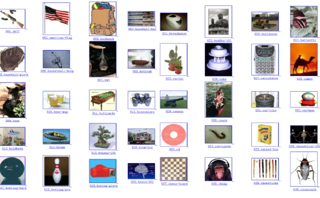
According to the number of nouns in the human languages, there are at least 10,000 to 30,000 object categories in the world [9]. However, at present machines can only recognize a few of them. For instance, to our best knowledge, in the computer vision community, the biggest public dataset for object recognition is Caltech-256 [30], which consists of 256 object categories plus a background category. Fig. 1.11 shows 40 samples from the first 40 categories in Caltech-256, one sample per category. So far the best recognition rate on this dataset is only about 50% [24], whereas for humans these objects can be categorized very easily. Therefore, much more effort is still needed for object recognition, and its breakthroughs will bring great benefit to other relative research such as video surveillance, navigation, etc.

1_{These images are extracted from}

http://www.vision.caltech.edu/Image_Datasets/ Caltech256/images/, where the samples of all the categories are shown.

(15)

CHAPTER 1. INTRODUCTION 2

Figure 1.1:40 samples from the first 40 categories in the Caltech-256, one sample per category.

Image similarityin this thesis is defined as an object based measure to show how likely two images contain the instances within the same object category, and a higher image sim-ilarity indicates a higher probability. Based on this measure, a perfect recognition can be made if the similarities of images which contain the same-category objects are higher than those of images which contain objects in different categories.

Considering that each object can be decomposed into smaller pieces, and each smaller piece gives an evidence that this object probably appears, we propose to match the same-typefeatures in images so that the image similarities are maximized. Here, “same-type” means that the visual information in the features should be the same. For instance, all fea-tures come from Scale Invariant Feature Transform (SIFT) [45] descriptors. We believe that the maximization criterion is suitable to reflect the image similarities properly, because two

(16)

more-similar images are inclined to have a higher maximization value. Specifically, with or without consideration for the spatial configurations of features, we further propose con-strained global feature correspondence[70] andprobabilistic feature matchingapproaches, respectively, for matching purpose.

With the increase of the number of visual sources from images, we face another prob-lem, that is, how to combine these different visual information for object recognition. Given a set of pre-calculated kernels, each of which is generated by the same-type features, we propose another approach, calledAdaptive Multiple Kernel Learning, to learn an optimal kernel using the max-margin criterion. Unlike other multiple kernel learning (MKL) ap-proaches, our approach is based on a biconvex optimization technique involved with an arbitrary norm of kernel coefficients to search for local optima as the solutions, and its pa-rameters can be learned for all the object categories either separately or jointly. Therefore, the efficiency of our approach is much higher than the traditional convex optimization based MKL approaches, especially with many object categories.

The rest of the thesis is organized as follows. Chapter 2 gives some background for object recognition in computer vision. Chapter 3 presents our maximum similarity based feature matching approaches. Chapter 4 explains our adaptive multiple kernel learning approach for information combination. Finally, we conclude the thesis in Chapter 5.

(17)

Chapter 2 Background

Again, the purpose of this thesis is only recognizing the object categories in images with-out localization or detection. In general, the object categorization process can be simply summarized as follows:

I Representing objects. Anobject representationis a type of organization of low level features in images, which are extracted from the image information of texture, color, shape, etc., to represent objects. Usually, different algorithms have their own object representations.

II Learning object category models. Based on the object representations in the training images, the model learning algorithms can generate a visual model for each object category. A visual model (model for short) of an object category can reflect some characteristics of the category defined by the model learning algorithms.

III Recognizing object categories. After learning the visual models, corresponding recog-nition algorithms are employed to calculate the similarities between the objects and the categories. A higher value means more likely the image contains the objects within the categories.

In the rest of this chapter, we will review some background information in each step. Specifically, Section 2.1 reviews some widely used low level features, Section 2.2 presents

(18)

some image patch sampling techniques, Section 2.3 introduces some object representations, and Section 2.4 explains support vector machines (SVMs) for learning and recognition.

2.1 Low Level Features

Low level features (descriptorsfor short) are usually vectors describing the visual infor-mation (e.g. texture, color, edge, etc.) in images or smaller image parts (patches for short). A simple example of low level features is a vector of RGB pixel values, which describes the color information of the pixel. So far, many sophisticated local descriptors have been proposed, for instance, Scale Invariant Feature Transform (SIFT) [45], PCA-SIFT [34], Gradient Location-Orientation Histogram (GLOH) [48], Speeded Up Robust Features (SURF) [2], Shape Context (SC) [3] and Geometric Blur (GB) [6]. Since in our experiments, only SIFT, SC and GB are employed, we just introduce these three descriptors. SIFT descriptors are highly distinctive, and its basic idea is to describe the patches in a high dimensional vector using gradient orientation histogram. Empirically in [45], to generate a SIFT descriptor for a patch, first this patch is resized to 16*16 pixels, then divided into 4*4 cells where in each cell there are 4*4 pixels. After this, a gradient orientation histogram with 8 bins is generated for each cell. Finally, an 8*4*4=128 dimensional feature vector is created for each SIFT descriptor.

Shape Context descriptors aim to locate the distribution of other shape points over relative positions in a region around a pre-defined reference point (center for short) by spatial quantization. When generating an SC descriptor for each point, a polar coordinate system is employed where one dimension is log-distance, and the other is relative angle.

Geometric Blur descriptors are highly dependent on the extracted edges in images, and the basic idea is to capture the relationship of oriented edges in a region around a pre-defined reference point (center for short) using a polar coordinate system, similar to SC descriptors. The difference is that a weighting distribution (usually a Gaussian distribution) is applied to the sample points so that each sample point has its own weight for counting purpose. The closer the sample point to the center is, the higher its weight is.

Additional properties (e.g. scale-invariance and rotation-invariance) of a descriptor are decided by how the patch is detected and how the descriptor is calculated. For example,

(19)

CHAPTER 2. BACKGROUND 6

SIFT descriptors are born to be scale-invariant and rotation-invariant, because (i) the interest point for each SIFT descriptor is located as a local optimum on multiple scales of an image using Difference-of-Gaussian (DoG) by comparing each sample point to its eight neighbors in the current DoG image (spatial space) and nine neighbors in the scale above and below (scale space), and then the whole patch is re-scaled to16×16pixels, which results in scale-invariance; (ii) to guarantee its rotation-invariance, the orientations of a SIFT descriptor are assigned relative to the interest point orientations.Interest point orientationsare calculated based on the image gradient magnitudes and orientations at all the pixels, and assigned as the highest peak and the local peaks that are within 80% of the highest peak in a 36-bin weighted orientation histogram. For SC and GB descriptors, after locating the interest points and their orientations in images, the polar coordinate systems in both SC and GB descriptors can be centered at the interest points and aligned relative to the interest point orientations like SIFT descriptors so that both SC and GB descriptors can be scale-invariant and rotation-invariant.

2.2 Image Patch Sampling

Animage patch samplingtechnique is an image patch extraction strategy before generat-ing descriptors. In general, there exist several samplgenerat-ing techniques for object recognition, for example, dense sampling (e.g. [41]), random sampling (e.g. [43]), segment sampling (e.g.[31]), interest point sampling (e.g.[45]), etc.

Dense Samplingusually divides images into many same-size cells with specific struc-tures. Its advantages are that it can control the total number, centers and scales of the patches, and it can utilize the information of each image sufficiently by covering it using the patches. The major drawback of this strategy is that the extracted patches may not be distinctive enough for object recognition.

Random Samplingdecides the centers and scales of the patches randomly. Like dense sampling, it can control the total number of the patches. However, it cannot control the centers and scales of the patches, and it may not extract distinctive patches for objects.

Segment Sampling utilizes some segmentation techniques (e.g. normalized cut [57]) to extract patches. Its advantages are that it can control the total number of the patches to

(20)

a certain degree, probably locate some distinctive patches for objects, and probably utilize the image information sufficiently. However, it cannot control the positions and scales of the patches.

Interest Point Sampling employs some interest point (or region) detectors to locate the centers and scales of the patches. An interest point is a pixel location around which a patch with a specific scale is extracted. Its advantage is that it can locate the distinctive object patches in the images as many as possible. However, it cannot extract an arbitrary number of patches like dense sampling or random sampling (e.g. no interest points at all in images), cannot control the centers and scales of the patches, and cannot utilize the image information sufficiently.

In [50], the authors did some research on the effect of different sampling strategies for image classification. It is found that the single most important factor governing perfor-mance is the number of patches sampled from the test image and ultimately interesting point detectors cannot provide enough patches to compete, so random sampling gives equal or better classifiers than interest point sampling. And in [43], the authors compared the dense, random, and interest point sampling strategies in their experiments, and addressed that dense sampling, which yields the most number of patches, is the best. So in our exper-iments, we only adopt dense sampling for patch extraction regardless of scale-invariance.

2.3 Object Representations

Using different algorithms, objects can be represented in different ways, for instance, Set-of-Features models (SoFfor short,e.g.[10]), Bag-of-Words models (BoWfor short,e.g.[15]), part based models (e.g.[20]), hierarchical models (e.g.[19]), etc.

Set-of-Featuresmodels represent each image as a set of same-type feature vectors, and assume that these features are independent and at least one feature comes from the target objects. Notice that features here could be either low level descriptors (e.g. SIFT) or high level vector representations (e.g. BoW). SoF is quite flexible, no limits on the number or dimensionality of features, and thus it is quite suitable for the feature matching purpose.

Bag-of-Wordsmodels represent each image as a histogram of occurrences of the code-words in a pre-defined codebook to capture their distribution. A codebook is generated

(21)

from a collection of clusters of training descriptors, and acodewordis the center of a clus-ter. BoW maps each descriptor to an index in the codebook by searching for its nearest codeword, considers this codeword to appear once, and finally creates a histogram. Still, BoW assumes that the descriptors in each image are independent and at least one comes from the target objects. Impressively, the performances of this simple representation on many datasets for object recognition are very good (e.g.[60, 41, 44]).

Part basedmodels take the spatial relationship of the patches in images into account, and represent objects in a structured way. Usually, descriptors are still quantized using a codebook like BoW, and based on this representation the learning algorithms can learn distinctive object part structures, which makes this representation quite successful in object recognition and detection. However, the number of learned object parts is restricted to a very small number, otherwise the computational time is very high.

Hierarchical models represent objects by organizing their information into tree-like trackable structures. Notice that the information here is not limited to the descriptors ex-tracted directly from images, but it could be any high level information among the objects (e.g. semantics). Theoretically, more similar the images are, more likely they share more information in the hierarchy.

Due to the characteristics of our algorithms, in our experiments we employ SoF for maximum similarity based feature matching and BoW for adaptive multiple kernel learning.

2.4 Support Vector Machines

Support vector machines(SVMs) are a set of supervised learning algorithms for classifi-cation and regression based on the max-margin criterion. Supervised learningis used for generating mapping functions between inputs and their labels. Originally, an SVM is de-signed for binary-class cases, and its basic idea is to find a separating hyperplane which maximizes the scaled distance between its two parallel hyperplanes, that is, the margin. Notice that in an SVM, there is an assumption that the larger the margin is, the smaller the generalization error of the classifier will be.

Specifically, inbinary-classcases where only two classes exist, one positive one nega-tive, suppose the training data is{(x1, y1),(x2, y2),· · · ,(xn, yn)}wherexi(i= 1,2,· · · , n)

(22)

denotes an input vector and its correspondingyi (i = 1,2,· · · , n) denotes the class label

(“1” if positive, otherwise “-1”). Then in an SVM the separating hyperplane is defined as

hw, φ(x)i+b = 0and the two corresponding parallel hyperplanes arehw, φ(x)i+b = 1 for the positive class andhw, φ(x)i+b = −1for the negative class, wherew is the vec-tor perpendicular to the separating hyperplane,b is a scalar,φ(x)denotes the pre-defined input vector mapping function of the SVM, and h·,·i denotes the inner product operator. For classification, if a test vectorxt satisfies hw, φ(xt)i+b > 0, it will be classified as

a positive instance; otherwise, if it satisfies hw, φ(xt)i+b < 0, it will be classified as a

negative instance. An SVM tries to find the optimalwandbto maximize the margin. Since the margin in an SVM is always equal to _||w||2

2 no matter what input vectors are,

maximizing the margin is equivalent to minimizing||w||2, further, equivalent to

minimiz-ing||w||2

2. Therefore, an SVM primal formulation in the hard margin cases is defined in

Eqn. 2.1. Here,hard marginmeans that the training data can be classified perfectly without any classification error.

min w,b 1 2 kwk 2 2 (2.1) s.t. ∀i, yi hw, φ(xi)i+b ≥1

In practice, training data is hardly ever classified properly without any error. To allow the classification errors by relaxing the margin condition from hard margin tosoft margin, slack variablesξare introduced into the SVM formulation above and a soft margin SVM is defined in Eqn. 2.2, whereCis a pre-defined non-negative constant to control the trade-off between the margin and the classification errors.

min w,b,ξ 1 2 kwk 2 2 +C X i ξi (2.2) s.t. ∀i, yi hw, φ(xi)i+b ≥1−ξi ξi ≥0, C ≥0

Based on the Lagrange multipliers α, Eqn. 2.2 can be rewritten as a dual formulation as shown in Eqn. 2.3, andwandbcan be calculated using Eqn. 2.4 and 2.5, whereNS is

(23)

Notice thatk(xi,xj) = hφ(xi), φ(xj)iis an element of akernel, which is a definite

semi-positive matrix. Eqn. 2.3 can be solved using quadratic programming (QP).

max α X i αi− 1 2 X i,j αiαjyiyjhφ(xi), φ(xj)i (2.3) s.t. ∀i, 0≤αi ≤C, X i αiyi = 0 w=X i αiyiφ(xi) (2.4) b = 1 NS X i∈S yi− hw, φ(xi)i = 1 NS X i∈S " yi− X j∈S αjyjhφ(xi), φ(xj)i # (2.5)

In the multi-class cases, where more than two classes exist, in general there are two strategies to train an SVM based on the binary cases, that is, one-vs-one and one-vs-rest. GivenN classes, the one-vs-one strategy trains N(N₂−1) binary SVMs to distinguish any pair of classes, whereas the one-vs-rest strategy trainsN binary SVMs, one for each class. For classification, different criteria can be used, e.g. max-voting [33], max-margin [15], etc. Also, multi-class SVMs can be trained for all the class models simultaneously (all-in-one for short). For instance, Weston and Watkins [67] proposed a multi-class SVM as defined in Eqn. 2.6, whereyi = 1,2,· · · , N denotes the true class label forxi. Its basic idea is that

the decision margin between an input and its true class should be bigger than that between it and any false class.

min w,b,ξ 1 2 N X c=1 kwc k22 +C X i,c6=yi ξi,c (2.6) s.t. ∀i, c 6=yi, hwyi, φ(xi)i+byi − hwc, φ(xi)i+bc ≥1−ξi,c ξi,c ≥0, C ≥0

Hsu and Lin [33] compared the one-vs-one and one-vs-rest strategies, and addressed that their performances are highly dependent on the classification problem at hand, and in their experiments, one-vs-one is slightly better in most cases. Further, Demirkesen and Cherifi [17] compared the three strategies above for scene image classification, and drew a conclusion that the all-in-one strategy outperforms the other binary class based strategies based on their experiments.

(24)

Maximum Similarity Based Feature

Matching

In this chapter, we propose two feature matching approaches to maximize the similarities between images. We believe that the maximum image similarity is a good measure for ob-ject recognition because two images with similar obob-jects in the same categories are incline to have a higher maximum similarity than two images with objects in different categories. Fig. 3.1 gives an example to explain the basic idea of our maximum similarity based fea-ture matching approaches. By matching the patches in images, intuitively the maximum similarity between the two bike images should be higher than that between the upper bike image and the car image, because the two bike images contain similar bike instances, while the upper bike image and the car image do not. In this way, it can be inferred which images more likely contain the same-category objects by calculating pair-wise maximum image similarity, and object recognition can be carried out using some classifiers like K-nearest neighbors (KNN), support vector machines (SVMs), etc.

Accordingly we propose the following two feature matching criteria for maximizing im-age similarities: Section 3.1 explains a constrained global feature correspondence approach, Section 3.2 addresses a probabilistic feature matching approach. Finally Section 3.3 sum-marizes the chapter.

(25)

CHAPTER 3. MAXIMUM SIMILARITY BASED FEATURE MATCHING 12

Figure 3.1:Illustration of the intuition of the maximum similarity measure.

3.1 Constrained Global Feature Correspondence

In this section, we consider the feature correspondence task as a graph matching problem. Our approach tries to maximize a similarity objective function, consisting of not only the feature vectors but also the constrained global spatial structures of two sets of feature points, by a new polynomial-time approximate optimization algorithm. This algorithm allows ev-ery node in a smaller graph to potentially be linked with any node in a larger graph, and thus it can handle one-to-one, many-to-one, and no match cases. We test this approach on the “hotel” and “house” video sequences for feature matching, and our results are quite impressive.

3.1.1 Introduction

Feature correspondence aims to find a sequence of feature matching pairs between two feature sets to satisfy certain conditions. Finding a correct feature correspondence is dif-ficult, because in two sets of feature points (i) the descriptor for each point may be quite different, even for pairs of ground truth matching points; (ii) the locations of the points may be changed by translation, rotation, scaling, etc.; (iii) some points may appear in a set but disappear in the other set. In general, the computational complexity of the feature correspondence problem is NP-hard [26].

(26)

employed affine features to estimate the parameters for conjugate rotation. Dellaert et al. [16] applied a Markov Chain Monte Carlo approach to estimate the posterior distribution over all possible feature correspondences instead of best-one matching scheme. Torresani et al. [59] formulated the feature correspondence task as a graph matching problem by min-imizing an energy objective function based on the feature vectors andlocalspatial struc-tures. Similarly, Caetano et al. [13] utilized graph learning algorithms to improve feature correspondence accuracy based on local structures of the graphs.

We also consider the feature correspondence task as a graph matching problem. Specifi-cally, in order to maximize the number of the feature matching pairs, in this paper we define the feature correspondence task as follows:

Definition 1(Maximum Similarity Based Feature Correspondence). Given two sets of featuresA={a1,a2,· · ·,a|A|}with|A|features, andB={b1,b2,· · ·,b|B|}with|B|features

(|A| ≤ |B|), a maximum similarity based feature correspondence is defined as an asym-metric matching process from the smaller setAto the bigger setB so that (i) each feature inAappears at most once in the matching pairs to allow one-to-one, many-to-one, and no match cases, and (ii) the similarity betweenAandB is maximized.

Naturally, minimizing an energy function is equivalent to maximizing a similarity func-tion, and here we adopt similarity maximizafunc-tion, which involves not only the feature vectors but also their constrained global spatial structures (CGSS), to find the feature correspon-dence. For many feature correspondence cases, the object instances in images have their specific global spatial configurations, e.g. the configurations of their parts or the relative locations between them. In these cases, CGSS will be quite helpful because it is designed based on this type of global spatial structure information. Because of computational com-plexity, we propose a polynomial-time approximate algorithm using a greedy strategy to search for the maximum iteratively as well as handling the different matching situations.

3.1.2 Similarity Objective Function

Many research works suggest that for feature correspondence problems the best approach is to combine the feature vectors with structure information. However, most of them focus on

(27)

thelocalstructures of feature points (e.g.[59, 13]). Here, we introduce a new feature struc-ture calledconstrained global spatial structure(CGSS). For each feature point, a CGSS is constructed by the normalized distances and the normalized angles between all the matched features in the matching sequence, and thus the CGSS is less sensitive to geometric trans-formations,i.e.translation, rotation and scaling. Further, we take the similarities between CGSS as a part of our similarity measure defined in Eqn. 3.1 for matching feature points between setAand setB, and the optimal feature correspondence is the one that maximizes the similarity betweenAandB, as defined in Eqn. 3.2.

S(A, B) = |A| X i=1 Si = |A| X i=1 k(vi|f)wk(si|f)1−wp(f) (3.1) F(A, B) = arg max f S (A, B) (3.2)

Here, _S(A, B) ∈ [0,1]and_F(A, B)respectively denote the similarity and the optimal feature correspondence between setAand set B (|A| ≤ |B|),f denotes any possible fea-ture correspondence,v denotes a feature vector, sdenotes a CGSS determined byf, p(f) denotes the prior knowledge of occurrence off modeled as a uniform distribution,k(vi|f)

andk(si|f)denote the feature similarity and structure similarity of theithmatching pair in

f, whose multiplication is proportional to the similarity score of the matching pair,Si, and

w(0≤ w≤ 1) is a parameter controlling the trade-off between the two similarities forSi.

In general, structurescan be designed based on different purposes, and in our algorithm we design it as the normalized distances and the normalized angles between the feature points, as illustrated in Fig. 3.3 fora1 andb2.

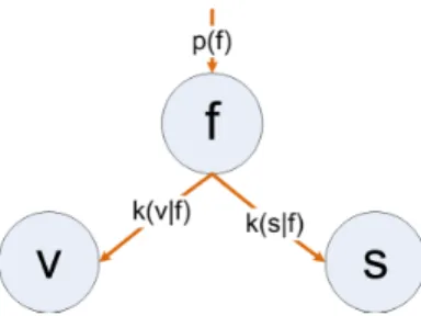
The intuition of multiplication of the feature similarity, the CGSS similarity, and the fea-ture correspondence occurrence prior is inspired by the graphical model shown in Fig. 3.2, where the feature matching pairvand their corresponding CGSSscan be considered as two attributes off, and the probability of co-occurrence of f, s andv is the multiplication of

p(f),k(v|f)andk(s|f). Since in our formulation the values of the feature similarities and the structure similarities are between 0 and 1, we simply take similarity as the equivalence of probability.

In [5], Berg et al. proposed a similar formulation to ours for finding feature correspon-dence. However, the major difference between these two formulations is that in [5] the

(28)

Figure 3.2: Intuition of multiplication of the feature similarity, the global feature structure similarity, and the feature correspondence occurrence prior.

feature structure cost is pair-wise, two features per set, and the mapping between these fea-tures from one set to the other defines the structure cost; whereas in our approach, the CGSS is defined based on all the previous matched features in a set, not limited to pair-wise. In other words, the definitions of feature structures in these two formulations are quite differ-ent, and to our best knowledge, introducing theconstrained global spatial structure (CGSS) similarityinto the matching process is novel.

3.1.3 Approximate Algorithm for Maximization

Notice that our similarity function is convex, and therefore its maximization is unique given set A and set B. However, this function is difficult to maximize because the CGSS s is related to all the matched feature points in the feature set. One way forward is to apply an exhaustive search to all possible feature correspondences, but its computational complexity is too high, given byO(₍_|_B_|−||B_A|!_|_+1)!).

Inspired by the Markov Chain Monte Carlo (MCMC) technique, we propose a polynomial-time approximate algorithm to increase the similarity score monotonically and iteratively. Basically, there are two steps in our algorithm: initialization and re-matching.

Initialization

The goal of the initialization is to select a good candidate forf from all possible candidates available for searching for the maximum so that the computational time is reduced. In this

(29)

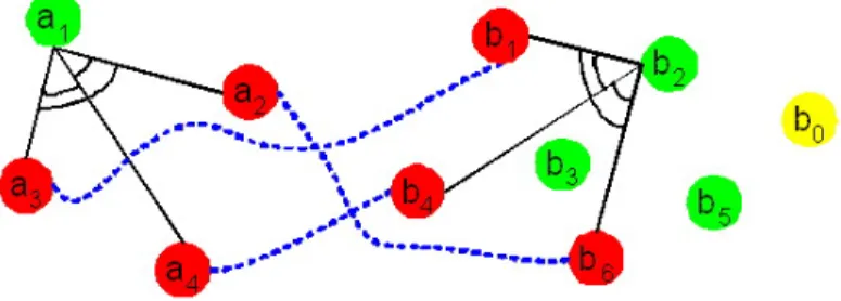
Figure 3.3: An example of feature correspondence between setAwith 4 points and setB with 6 points. Here, green dots represent the unmatched points in each set, red dots represent the matched point pairs con-nected by blue dotted lines, and the yellow dotb0is for no match cases which does not belong toB. The constrained global spatial structure for pointa1(reps. b2) consists of the normalized distances and the nor-malized angles betweena1(reps.b2) and each matched point in the set.

step, we tentatively match the feature points inA and B such that each point in A has a match inB, since|A| ≤ |B|. Here, we utilize the Iterated Conditional Modes (ICM) [7] criterion for initialization.

Specifically, ICM allows a point pair, which has the maximum similarity scoreSbased on the matched pairs before, to be added into the current matching sequence in each itera-tion. We describe each selection process as follows:

fi = arg max

ˆ

fi

k(vi|fˆ)wk(si|fˆ)1−wp( ˆf) (3.3)

where fi (i = 2,3,· · · ,|A|) denotes the ith point pair which is added into the current

matching sequence fˆconsisting of i− 1 point pairs, and fˆi denotes any possible point

pair candidate. Other variables have the same meanings as those in Eqn. 3.1. For the first matching pair infˆ, we simply add the one with the maximum feature similarity intofˆ.

Example 1 (Initialization). In Fig. 3.3, suppose we have matched 3 point pairs (red dots) be-tweenAandB, and would like to find a match fora1 amongst b2, b3, and b5 (green dots). Now

we calculate the similarity score betweena1 andb2. Their feature similarityp(vi|fˆ)is calculated

directly based on their feature vectors. Theconstrained global spatial structure(CGSS) ofa1is (1)

the normalized distances, which are the normalization of the distances betweena1 anda2,a3,a4;

and (2) the normalized angles, which are the normalization of the angles betweena1and any pair of

(30)

k(si|fˆ)can also be calculated directly. Notice that for each point, the CGSS has its own order, and

these orders must be consistent with each other. For instance, if the order of the normalized distances fora1 isha1, a2i, ha1, a3iandha1, a4i, then forb2 the calculation order must behb2, b6i,hb2, b1i

andhb2, b4i. It is similar for calculating the normalized angles. Thus, using Eqn. 3.3 the similarity

score for the paira1andb2can be calculated easily. After finishing the calculation of the similarity

score for each candidate pair, we select the pair with the maximum asfi. In sum, our approximate

matching optimization allows including a measure of global spatial information without the penalty of an exhaustive or another slow search.

Re-matching

After initialization, we re-match each point inAwith the points in B iteratively, using the exhaustive search while keeping the other pairs in the current feature correspondence f

unchanged, so that the similarity defined by Eqn. 3.1 will increase. We maintain the current global structure by re-mapping a single node in turn whilst keeping the graph unchanged, and thus impose severe consistency constraints. The purpose of this step is to correct any “wrong” matching pair. In this process, we add a new point b0 (yellow dot) into B for

handling the no match cases, as illustrated in Fig. 3.3. When a point inAmatchesb0, the

similarity score of this pair is equal to 0, and if in this case the similarity of the matching sequence increases, then that point should have no matching point inB currently. In other cases, we calculate the similarity score for each pair of the point candidates, and when we find a new point correspondence which increases the similarity of the matching sequence, we update the matching sequence and its similarity score. In this way, our re-matching process can handle the one-to-one, many-to-one and no match cases.

Example 2 (Re-matching). In Fig. 3.3, suppose after initialization the feature correspondence isha1, b5i,ha2, b6i,ha3, b1iandha4, b4i, and the corresponding similarity of this feature

correspon-dence iss0. Now we would like to re-matcha1with any point inBplusb0so thats0can increase.

Suppose we try to matcha1 withb2; then to calculate the similarity betweena1 andb2, we keep

the other matched pairsha2, b6i,ha3, b1iandha4, b4iunchanged, and calculate the normalized

dis-tances and the normalized angles betweena1 anda2,a3,a4 fora1, and betweenb2 andb1,b4, b6

forb2. This calculation is repeated forha2, b6i,ha3, b1iandha4, b4irespectively, and using Eqn. 3.1

(31)

ha4, b4i, denoted ass1. Ifs1 > s0, then we update the feature correspondence to be the current one

along with its similarity, and otherwise keep searching. Overall, this is a highly constrained and fast method.

As an approximation algorithm, we also enforce each increase amount to be no less than

( >0), with our algorithm terminating if there is no such increase amount in|A|(|B|+ 1)

searches. Since our global feature structure similarities are highly dependent on the previ-ous matched feature pairs, our approximation algorithm may be stuck in local solutions due to the greedy strategy. Therefore, a good feature correspondence candidate in the initializa-tion stage will be quite useful, not only for avoiding local soluinitializa-tions but also for reducing computational time. Below is a proposition which proves that our approximate algorithm is polynomial-time.

Proposition 1. The computational complexity of our approximate optimization algorithm isO(|A|2_|_B_|₎₍_|_A_{| ≤ |}_B_|_).

Proof. LetSmaxandSinitdenote the maximum ofS(A, B)and its value after initialization,

and suppose that inT searches the maximum increase amount∆Sis found. Then because

Smax ≤ |A|, Sinit ≥0,T ≤ |A|(|B|+ 1), and∆S ≥, we can estimate the computational

complexity of our approximate algorithm as follows.

O (Smax−Sinit)T ∆S ≤O |A| · |A|(|B|+ 1) =O(|A|2_|_B_|₎

Thus, our approximate algorithm is polynomial-time.

To summarize our algorithm, we show the pseudo code of our algorithm in Alg. 3.1.

3.1.4 Experiments

We tested our approach on the “hotel” video sequence1 used in [59, 13] consisting of 101 frames of a toy hotel, and the “house” video sequence2used in [13] consisting of 111 frames

1_{This sequence is downloaded from} _{http://vasc.ri.cmu.edu/idb/html/motion/hotel/}

index.html.

2_{This sequence is downloaded from} _{http://vasc.ri.cmu.edu/idb/html/motion/house/}

(32)

Algorithm 3.1: Polynomial-time Approximate Algorithm for Maximization Input: setA, setB

Output: feature correspondence_F

Initialize_Fbased on Iterated Conditional Modes (ICM) using Eqn. 3.3 so that each feature inAappears once in the matching pairs;

repeat

Calculate the similarityS for a possible matching pair using Eqn. 3.1; if_S(A, B)increasedthenUpdate_F;

elseContinue to search exhaustively; untilNo increase of_S(A, B)exists; return_F

of a toy house. We employed the Shape Context3[4] descriptor to generate a feature vector for each point. To measure the similarity of two feature vectors or their corresponding CGSS, we used the RBF-kernel with theχ2distance. For instance, given two feature vectors

v1 andv2withddimensions, their feature similarityk(v1, v2)is defined in Eqn. 3.4.

k(v1, v2) = exp ( − d X i=1 (v1,i−v2,i)2 v1,i+v2,i ) (3.4)

In our experiments, for each sequence we take as ground truth4_{the same 30 point-pairs}

as in [59, 13]. Our goal is to find the feature correspondence between two frames with frame intervalk, wherek ∈ {25,15,10,5,3,2}. That is, the frame-order distance between two frames in the sequence is equal tok. For example, if k = 2, we will find the feature correspondence for the frame pairs with order(1,3),(2,4),· · ·,(N−3, N−1),(N−2, N), whereN is the total number of the frames in the sequence.

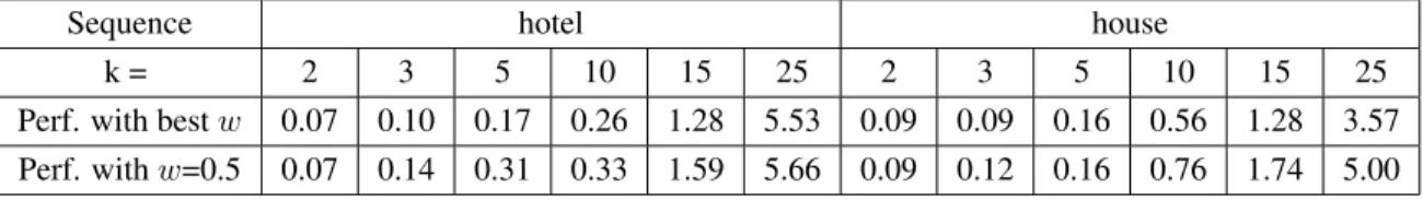
We fixed the parameter to 0.02 during all the experiments, and tested our approach using different values of w from 0 to 1 step by 0.1 on the two sequences, as shown in Fig. 3.4 for “hotel” (left) and “house” (right). Clearly (and unsurprisingly) our approach works better with smallerk: whenk = 2our best results are 0.07% for “hotel” and 0.09% for “house”, truly excellent results. Whenk = 25 our best results are 5.53% and 3.57%,

3_{Since in [59, 13] Shape Context is employed, we also use it. Other descriptors can be also utilized here.} 4_{We appreciate help from Drs. Lorenzo Torresani and Vladimir Kolmogorov in providing us with}

(33)

(a) Hotel (b) House

Figure 3.4: Mismatching percentages (%) vs. parameterwusing differentkintervals for (a) “Hotel” and (b) “House” sequences.

Table 3.1: Performance comparison betweenw= 0.5and the bestwfor differentkintervals (%).

Sequence hotel house

k = 2 3 5 10 15 25 2 3 5 10 15 25

Perf. with bestw 0.07 0.10 0.17 0.26 1.28 5.53 0.09 0.09 0.16 0.56 1.28 3.57 Perf. withw=0.5 0.07 0.14 0.31 0.33 1.59 5.66 0.09 0.12 0.16 0.76 1.74 5.00

respectively, as listed in Table 3.1. This is quite reasonable, because whenk is small, the relative positions of the points are little changed, leading to a better description of Shape Context and more similarity of the CGSS of points, compared to largerk. Even fork = 25, a very wide gap in time, the results are quite respectable.

Also we make another two observations: (i) The errors first decrease fromw = 0and then increase when wis close to 1, with the best results forw around 0.5. This indicates that both feature vectors and their corresponding CGSS contribute to finding the optimal feature correspondence; (ii) Aroundw = 0.5, all the lines are relatively flat, which means in that range the performance of our approach is less sensitive to the changes inw. There-fore, inferred from these two sequences, our approach needs no training data in order to select optimal value forw, and we can simply fixw= 0.5when we do not have any prior knowledge about the data, since fixingwis the only learning aspect to the algorithm. For these two sequences, we compare performance withw = 0.5to the best performance, in Table 3.1. From the table, we see that the differences are quite small between a fixed w

(34)

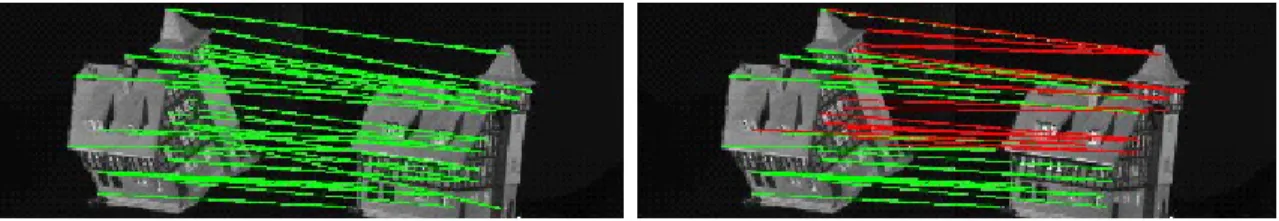
Figure 3.5: Our result for matching the first and last frames (k = 100) of the “hotel” sequence, where green lines indicate the correct feature correspondences, and the red lines indicate the wrong ones. Left: Ground truth of the feature correspondences predefined in the two images. Right: Our result (accuracy: 14/30 = 46.7%) withw= 0.5.

Figure 3.6: Our result for matching the first and last frames (k = 110) of the “house” sequence, where green and red lines have the same meanings as Fig. 3.5. Left: Ground truth of the feature correspondences predefined in the two images.Right: Our result (accuracy:12/30 = 40.0%) withw= 0.5.

and the bestw. Also, these results are comparable to those in [59, 13], although we cannot directly compare since the values ofk for frame pairs are not stated there. Comparing the computational time, on average for matching a frame pair based on our Matlab implemen-tation without any optimization, it takes 1.24 and 1.22 seconds on “hotel” and “house”, respectively, on a 2.33GHz Core 2 Duo CPU, while in [59] their “DD” approach needs nearly 30 seconds.

We also tested our approach to find the feature correspondence between the first and lastframes in each sequence — a very challenging test. Here we used a constantw = 0.5. The results are shown in Fig. 3.5 for “hotel” (k = 100) and Fig. 3.6 for “house” (k= 110), where the correspondence accuracies are 14/30 = 46.7% and 12/30 = 40.0% for “ho-tel” and “house”, respectively. This is because the changes of the relative positions of the points make it difficult for the Shape Context descriptor to identify the same points. How-ever, compared with the result of the linear assignment without learning in [13] for “house” (7/30), we have achieved significant improvement. Although the matching accuracy of the

(35)

constrained global feature correspondence approach is respectable, some issues make it dif-ficult to apply this approach to object recognition on large-size datasets,e.g. its asymmetric matching and scalability, and we do not perform any experiment on object recognition using this approach.

3.2 Probabilistic Feature Matching

In this section we propose another novel feature matching approach called Probabilistic Feature Matching(PFM). We consider the matching process as the bipartite graph match-ing problem, and define the image similarity as the inner product of the feature similari-ties and their corresponding matching probabilisimilari-ties, which are calculated by optimizing a quadratic formulation. Further, we prove that the image similarity and the sparsity of the feature matching probability distribution will decrease monotonically with the increase of parameter C in the quadratic formulation where C ≥ 0 is a pre-defined data-dependent constant. Essentially, our approach is the generalization of a family of similarity measure-ment approaches. We test our approach on Graz datasets for object recognition, and achieve 89.4% on Graz-01 and 87.4% on Graz-02, respectively on average.

3.2.1 Introduction

We consider each image as an undirected graph and take the feature matching process as the bipartite graph matching problem as illustrated in Fig. 3.7, where any pair of features from two images could be possibly matched.

Different strategies can be utilized in the feature matching process. Lyu [46] introduced the Summation Kernel (SK) to measure the image similarities as follows:

Ksum(V1, V2) = X vi∈V1 X vj∈V2 k(vi, vj) (3.5)

whereV1 (resp. V2) denotes a feature set,vi ∈ V1 (resp. vj ∈ V2) denotes a feature vector

(36)

Figure 3.7: Illustration of matching two images. Each image is represented as a collection of features of the patches. Weights (red) on the edges (green) denote the matching probabilities between the feature pairs so that the similarity between the two images is obtained.

sections, we denote k(vi, vj) as kij for short. Wallraven et al. [65] proposed the

Max-selection Kernel (MK) as shown below:

Kmax(V1, V2) = 1 2    X vi∈V1 max vj∈V2 kij + X vj∈V2 max vi∈V1 kji    (3.6)

Fr¨ohlichet al.[22] proposed the Optimal Assignment Kernel (OAK) to maximize the simi-larity score between two structured objects by finding exactly one-to-one matches between the parts of these objects, defined as follows:

KOA(x, y) = ( maxπ P|x| i=1k(xi, yπ(i)) if|y|>|x| maxπP |y| j=1k(xπ(j), yj) otherwise (3.7)

wherex(resp.y) denotes an object,xi(resp. yj) denotes a part ofx(resp. y),|x|(resp. |y|)

denotes the total number of the parts ofx(resp. y), andπdenotes a permutation of parts. In contrast, the novel contribution of this approach is that we introduce a probabilistic matching strategy into the matching process as illustrated in Fig. 3.7, and we show that our approach can be considered as the generalization of a family of similarity measurement

(37)

approaches, including SK, MK, and OAK, so that the similarity can be decided adaptive to the data. In our approach, the similarity between two images is defined as the inner product of their feature similarities and the corresponding feature matching probabilities, which are calculated by optimizing a quadratic formulation.

3.2.2 Image Similarity Function

Given two images X = {x1,· · · , x|X|} and Y = {y1,· · · , y|Y|}, where xi ∈ X (resp.

yj ∈ Y) denotes a feature inX (resp. Y) and |X|(resp. |Y|) denotes the total number of

features inX (resp.Y), according to the bipartite graph matching problem, their similarity can be defined as follows:

S(X, Y;α,k) = |X| X i=1 |Y| X j=1 αijkij (3.8)

whereαij denotes thefeature matching probability(FMP) between featuresxi andyj, kij

denotes their similarity, andS(X, Y;α,k)denotes the similarity between X andY given the feature matching probability functionα(see Section 3.2.3 for details) and their feature similarity matrixk.

3.2.3 Feature Matching Probability Function

Intuitively, an FMPαij can be utilized to describe how likely featurexiandyj are matched.

As illustrated in Fig. 3.7, the axle with black circle on the left has 0.8 FMP with the axle with black circle on the right, while it has 0.2 FMP with the background feature, which is quite reasonable. Therefore, by considering the matching process as a function, we propose a very useful concept, called feature matching probability function, and give its definition as follows:

Definition 2(Feature Matching Probability Function). Given two imagesX={x1,· · · , x|X|}

and Y={y1,· · · , y|Y|}, a feature matching probability function (FMPF) α is defined as

α : X×Y → n{0}S

R+

o

|X|×|Y|, where R

+ _{denotes the field of positive real numbers.}

(38)

H ⊆ {−→x ,−→y}fromα, each FMPF will correspond to a point in the vector space covered by the following convex set:

( α| X ∀h∈H α1, X i,j αij = min (|X|,|Y|), 0α1 )

where “” denotes the element-wise operator of “≤”.

Notice that if H = ∅, the first constraint in the convex set above does not apply. In the constraint set ofα, the first constraint guarantees that the total matching probability of eachcorresponding feature is no more than 1, the second constraint guarantees that the total matching probability ofallthe features is equal to the total number of features in the smaller set, and the last constraint guarantees that each element inαrepresents a probability.

Actually, we can use this concept to describe the matching processes in SK, MK, and OAK. Specifically, (i) in SK any pair of features could be matched and their matching weight is fixed as 1, soα can be modeled as a uniform distribution; (ii) in MK a unique feature is selected as a match for every feature in both feature sets and their matching weight is fixed as 1, others 0, totally|X|+|Y|matched feature pairs; (iii) in OAK each feature in both sets can occur in the matched feature pairs at most once with the matching weight equal to 1, others 0, totallymin{|A|,|B|}matched feature pairs. In these approaches, the weights are pre-defined and kept the same during the matching process, no matter what the data is. In our approach, α is calculated automatically by optimizing a quadratic formulation so thatα can be adaptive to the different data, which could reflect the matching relationship between features better. As a result, our approach can be considered as the generalization of SK, MK, and OAK as explained in next section.

3.2.4 Probabilistic Feature Matching Optimization

We would like to perform the probabilistic feature matching between two images auto-matically. Therefore, we propose a quadratic optimization formulation [49] as defined in Eqn. 3.9 to calculateα, wheref(α;C)denotes our objective function,αis the only variable,

(39)

Cis a pre-defined non-negative constant, andkis the feature similarity matrix.

max α f(α;C) = X i,j αijkij−C X i,j α2_ij (3.9) s.t. X ∀h∈H α1,X i,j αij = min (|X|,|Y|),0α1, C ≥0

In our objective function, the first part is to measure the image similarity, the second part is to measure the sparseness of the distribution ofα, andC ≥ 0is a pre-defined data-dependent constant to control the trade-off between the two parts. Usually,sparsenessis a measure from_Rnto_Rfor a vector to quantify how much energy is actually packed into only a few components [32]. In our case, since the total energy is fixed, we define the sparseness of a distribution as the variance of the distribution. Therefore, to minimize the sparseness ofα, we have

minnSP(α)o= minnV ar(α)o= minnE[α2]−E[α]2o⇔minnE[α2]o (3.10)

whereSP(·)denotes the sparseness of a distribution, andE[·]andV ar(·)denote the mean and variance operators.

In order to see the relationship between our approach and some other similarity mea-surement approaches, we need the following important theorems on convexity [49]:

Theorem 1. Consider maxf(x) over x ∈ X, where f(x) is convex, and X is a closed convex set. If the optimum exists, a boundary point ofX is the optimum.

Theorem 2. If a convex functionf(x)attains its maximum on a convex polyhedronX with some extreme points, then this maximum is attained at an extreme point ofX.

Based on the theorems above, we can show that in certain cases our approach can be considered as equivalences to SK, MK and OAK by choosing differentCandHin Eqn. 3.9.

• C = +∞ and H = {−→x ,−→y}: According to Thm. 1, the optimized α in Eqn. 3.9 will be a uniform distribution, that is,αij = _max(_|_X1_|_,_|_Y_|₎, and by re-scalingαto1, our

approach can be considered as an equivalence to SK [46].

• C = 0andH={−→x ,−→y}: According to Thm. 2, the optimizedαin Eqn. 3.9 will sim-ulate a one-to-one matching process without feature re-occurrence, and our approach is equivalent to OAK [22].

(40)

• C = 0andH={−→x}: According to Thm. 2, the optimizedαwill simulate the match-ing process that selects the biggest similarity along the−→x-dimension for each feature in the−→y-dimension, and the corresponding similarity is equivalent toP

jmaxikij in

Eqn. 3.6. Thus, by optimizing Eqn. 3.9 along the−→x and−→y-dimension ofα, respec-tively, our approach is equivalent to MK [65].

Moreover, our approach has the following property:

Proposition 2. For two images X and Y, both the sparseness of α and their similarity

S(X, Y;α,k)will decrease monotonically with increasingC in Eqn. 3.9.

Proof. Considering C1 > C2 ≥ 0 and their corresponding α1 and α2 calculated using

Eqn. 3.9, we havef(α1;C1) ≥ f(α2;C1) and f(α2;C2) ≥ f(α1;C2). Putting them

to-gether, we have

C1α02α2−C1α10α1 ≥α02k−α

0

1k≥C2α02α2−C2α01α1 (3.11)

whereα1,α2 andkare vectorized, and0denotes the transpose operator. Then we get

(C1−C2)(α20α2−α01α1)≥0 (3.12)

SinceC1 > C2 ≥ 0, thenα01α1 ≤ α02α2, which indicates that a smallerC will lead to anα

with larger sparseness. Besides, we have

S(X, Y;α2,k)−S(X, Y;α1,k) = α02k−α

0

1k≥C2(α02α2−α01α1)≥0 (3.13)

Therefore,S(X, Y;α,k)will decrease monotonically with the increase ofC.

This property simplifies the adjustment of C in the cross-validation for different data so that our approach can be adaptive to the data. For instance, based on this proposition and the optimization of Eqn. 3.9 in both−→x and −→y-dimension of α, we know that when

C = +∞the similarities between images are the smallest (equivalent to the normalization of SK) and whenC = 0their similarities are the biggest (equivalent to OAK). By increasing (or decreasing) the value ofCmonotonically using the cross-validation techniques, we can find a good parameter value for the recognition purpose.

(41)

3.2.5 Classification with Support Vector Machines

In general, there is no guarantee that the similarity matrix generated by our approach is a valid kernel, whereas theoretically support vector machines (SVMs) are utilized with ker-nels for classification. However, in practice, an arbitrary similarity matrix can be involved in an SVM by adding a small positive number to the entries along the diagonal when it is not valid (e.g.[69]), as did in Eqn. 3.14, where|λmin|denotes the absolute value of the

minimum eigenvalue of the similarity matrixK, andIdenotes the identity matrix.

K0 =K+|λmin|I, ifλmin <0 (3.14)

3.2.6 Experiments

We tested our approach on the Graz-01 [51] and Graz-02 [52] datasets to perform the “ob-ject & non-ob“ob-ject” binary classification, with performance measured by Equal Error Rate (EER). Graz-01 is a challenging dataset with two object categories (bike: 373 images, per-son: 460 images) and a background category (270 images), because they vary greatly in object scale, pose and illumination. Compared to Graz-01, Graz-02 can be considered as an improved version with much more challenge, and comprises 3 object categories (bike: 365 images, person: 311 images, car: 420 images) and a background category (380 images). The size of each image in both datasets is either 640×480 or 480×640 pixels.

In our experiments, all the images were converted into gray scale, and we utilized the dense sampling technique [60] to sample the images so that each patch consists of 10×10 pixels. For each patch, we employed the SIFT [45] descriptor to represent it, and then used K-means to generate a codebook with 200 codewords so that each descriptor can be represented by the closest codeword in the feature space. Finally, by counting the occur-rence of each codeword in the cells of the 3×3 grid, we created 9 histograms to represent each image. The RBF-kernel withχ2 distance was used to compare the similarity of two histograms, that is,

kij = exp ( − d X n=1 (vi,n−vj,n)2 vi,n+vj,n ) (3.15)

wheredis the number of dimensions of histogramsviandvj. The regularization parameter

(42)

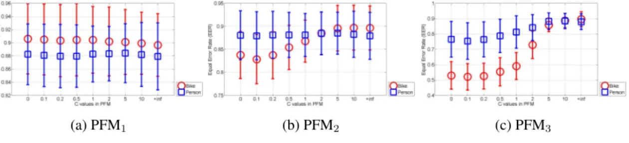
(a) PFM1 (b) PFM2 (c) PFM3 Figure 3.8:Performance comparison on Graz-01 between different PFM with differentC.

the notations, we use PFM1, PFM2 and PFM3 to denote our approach withH = {−→x ,−→y},

H={−→x}orH ={−→y}, andH =∅, respectively.

Graz-01

Table 3.2: Comparison results between different approaches on Graz-01 (%)

Bike Person Ave.

SPK [41] 86.3±2.5 82.3±3.1 84.3 PDK [44] 90.2±2.6 87.2±3.8 88.7 PFM1(C=0) 90.6±5.3 88.2±4.6 89.4

PFM2(C=5) 89.6±4.9 88.5±4.6 89.0

PFM3(C=+∞) 89.6±4.8 87.9±5.1 88.8

For the training-test data selection, we followed the setup in [41]. Specifically, we randomly selected 100 images in the positive class and 50 in each negative class (including the background) as our training set, and performed the test on similarly distributed data sets consisting of half the number of the training images per category.

Fig. 3.8 shows our performance on Graz-01. In general, PFM1 performs best, while

PFM3 performs worst, and PFM1 is much more stable with the increase of C than the

others. We also list the best performance of each PFM in Table 3.2 and compare them with some other published results. Clearly, all of our results outperform them.

Graz-02

We followed the experimental setup in [52] for the training-test data selection. Specifically, for each object category, we randomly selected 150 positive and 150 negative (50 for each

(43)

(a) PFM1 (b) PFM2 (c) PFM3

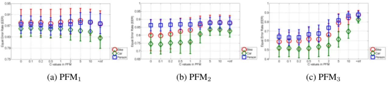
Figure 3.9:Performance comparison on Graz-02 between different PFM with differentC.

Table 3.3: Comparison results between different approaches on Graz-02 (%) Bike Person Car Ave.

Boost.+SIFT [52] 76.0 70.0 68.9 71.6 Boost.+Comb. [52] 77.8 81.2 70.5 76.5 PDK+SIFT [44] 86.7 86.7 74.7 82.7 PDK+hybrid [44] 86.0 87.3 74.7 82.7 PFM1+SIFT (C=5) 88.9 88.1 85.2 87.4 PFM2+SIFT (C=10) 88.0 87.9 83.6 86.5 PFM3+SIFT (C=+∞) 87.7 87.8 82.6 86.0

non-object class, including the background) images as the training data, and selected 75 positive and 75 negative (25 for each non-object class, including the background) with similar distribution of the training data as the test data, respectively.

Fig. 3.9 shows our performance on Graz-02. Compared to Fig. 3.8, similar observations can be made. Therefore, H = {−→x ,−→y} seems the best choice among the three for our PFM. Also, Table 3.3 lists the best results using different PFM in comparison with some other published results, and all of ours outperform them significantly.

3.3 Summary

In this chapter, we propose two different criteria for matching the same-type features in images to maximize their similarities.

First, we formulate the feature correspondence task as a graph matching problem, and propose a similarity function involving both feature vector similarities as well as corre-sponding constrained global spatial structure similarities. That we can include this global

(44)

structure information in optimal feature correspondence is due to the introduction of a new polynomial-time approximation maximization algorithm, which updates the similarity score iteratively. While allowing many potential matches, the update is strictly constrained by the global structures of features, making for a fast algorithm compared to some state-of-the-art graph matching algorithms with comparable accuracies as demonstrated by our experiments.

However, this approach defines an asymmetric matching process which limits its ap-plication in object recognition, particularly on large-size datasets. Therefore, we propose another novel feature matching approach called probabilistic feature matching (PFM). In this approach, the similarity between two images is defined as the inner product between the feature similarities and their corresponding matching probabilities, which are calcu-lated data-dependently by solving a quadratic optimization problem. We also prove that the image similarity and the sparseness of the feature matching probability distribution will de-crease monotonically with the inde-crease of parameterCin the quadratic formulation. Essen-tially, our approach is the generalization of a family of similarity measurement approaches, including the Summation Kernel, the Max-selection Kernel, and the Optimal Assignment Kernel. In our experiments, we tested our approach on Graz datasets for object recognition. On average, we achieved 89.4% on Graz-01 and 87.4% on Graz-02, respectively.

(45)

Chapter 4 Adaptive Multiple Kernel Learning

Usually humans recognize objects based on their different sources of information rather than one [18]. Recently, impressive accuracies for object recognition in images have been achieved on several benchmark datasets by combining multiple sources of object informa-tion. In this chapter, we propose a novel multiple kernel learning (MKL) approach, called Adaptive Multiple Kernel Learning(AdaMKL)1, for information combination based on the max-margin criterion. Unlike other traditional MKL approaches, our objective function is defined as a family of biconvex functions with an arbitrary`p-norm (p ≥ 1) of kernel

coefficients to learn the weights for support vectors and the kernel coefficients at a local op-timum. In our learning algorithm, AdaMKL minimizes our objective function alternatively by updating some variables while fixing the others at a time, where only one convex for-mulation needs to be solved. Besides, AdaMKL is suitable for either binary-class learning or multi-class learning. These characteristics make the learning of AdaMKL much more efficient.

We test our approach on the Caltech datasets for object recognition. Our experiments demonstrate that training AdaMKL is much (at least 10 times) faster than training some convex optimization based MKL algorithms with better accuracies. On Caltech-101, our mean category accuracies are(67.2±1.4)% and (74.4±0.5)%using 15 and 30 training images per category, respectively, and on Caltech-256, ours are(31.4±1.0)%and(36.4±

1_{Part of this work has been accepted by ICPR’10 [71].}

Maximum similarity based feature matching and adaptive multiple kernel learning for object recognition

MAXIMUM SIMILARITY BASED FEATURE

MATCHING AND ADAPTIVE MULTIPLE KERNEL

LEARNING FOR OBJECT RECOGNITION

1../0

---,--b

r

d

~

2-01'0

Declaration of

Partial Copyright Licence

Contents

List of Tables

List of Algorithms

Introduction

Chapter 2

Background

2.1

Low Level Features

2.2

Image Patch Sampling

2.3

Object Representations

2.4

Support Vector Machines

Maximum Similarity Based Feature

Matching

3.1

Constrained Global Feature Correspondence

3.1.1

Introduction

3.1.2

Similarity Objective Function

3.1.3

Approximate Algorithm for Maximization

3.1.4

Experiments

3.2

Probabilistic Feature Matching

3.2.1

Introduction

3.2.2

Image Similarity Function

3.2.3

Feature Matching Probability Function

3.2.4

Probabilistic Feature Matching Optimization

3.2.5

Classification with Support Vector Machines

3.2.6

Experiments

3.3

Summary

Chapter 4

Adaptive Multiple Kernel Learning

_r